Nonlinearity as a resource for nonclassicality

(1)

Scuola di Scienze

Corso di Laurea Magistrale in Fisica

Nonlinearity As a Resource for Nonclassicality

Relatore:

Prof. Cristian Degli Esposti Boschi

Correlatore:

Prof. Matteo G. A. Paris

Presentata da:

Francesco Albarelli

Sessione III

(2)

Lo scopo di questo lavoro è cercare un’evidenza quantitativa a supporto dell’idea idea che la nonlinearità sia una risorsa per generare nonclassicità. Ci si concentrerà su sistemi uni-dimensionali bosonici, cercando soprattutto di connettere la nonlinearità di un oscillatore anarmonico, definito dalla forma del suo potenziale, alla nonclassicità del relativo ground state.

Tra le numerose misure di nonclassicità esistenti, verranno impiegate il volume della parte negativa della funzione di Wigner e l’entanglement potential, ovvero la misura dell’entan-glement prodotto dallo stato dopo il passaggio attraverso un beam splitter bilanciato avente come altro stato in ingresso il vuoto. La nonlinearità di un potenziale verrà invece carat-terizzata studiando alcune proprietà del suo ground state, in particolare se ne misurerà la non-Gaussianità e la distanza di Bures rispetto al ground state di un oscillatore armonico di riferimento. Come principale misura di non-Gaussianità verrà utilizzata l’entropia relativa fra lo stato e il corrispettivo stato di riferimento Gaussiano, avente la medesima matrice di covarianza.

Il primo caso che considereremo sarà quello di un potenziale armonico con due termini polinomiali aggiuntivi e il ground state ottenuto con la teoria perturbativa. Si analizzeranno poi alcuni potenziali il cui ground state è ottenibile analiticamente: l’oscillatore armonico modificato, il potenziale di Morse e il potenziale di Posch-Teller. Si andrà infine a studiare l’effetto della nonlinearità in un contesto dinamico, considerando l’evoluzione unitaria di uno stato in ingresso in un mezzo che presenta una nonlinearità di tipo Kerr.

Nell’insieme, i risultati ottenuti con tutti i potenziali analizzati forniscono una forte evi-denza quantitativa a supporto dell’idea iniziale. Anche i risultati del caso dinamico, dove la nonlinearità costituisce una risorsa utile per generare nonclassicità solo se lo stato iniziale è classico, confermano la pittura complessiva.

Si sono inoltre studiate in dettaglio le differenze nel comportamento delle due misure di nonclassicità.

(3)

The aim of the present work is to find a quantitative evidence to support the idea that nonlin-earity is a resource to generate a nonclassicality. We will focus on unidimensional bosonic systems, mainly trying make a connection between the nonlinearity of an anharmonic os-cillator, defined by the functional form of its potential, and the nonclassicality of the corre-sponding ground state.

Among the many nonclassicality measures in existence, we will use the volume of the negative part of the Wigner function and the entanglement potential, that is the amount of entanglement obtained after the state goes through a balanced beam splitter, with the vacuum as the other input state. The nonlinearity of a potential is characterized by properties of the ground state, in particular its non-Gaussianity and the Bures distance from the ground state of a reference harmonic oscillator. To measure non-Gaussianity we will use the relative entropy between the state and the corresponding reference Gaussian state, the one with the same covariance matrix.

The first model under consideration will be a harmonic potential with two added poly-nomial terms and the ground state obtained with perturbation theory. We will then analyse three potentials with an analytical ground state: the modified harmonic oscillator, the Morse potential and the Posch-Teller potential. We will also study the effect of nonlinearity in a dynamical context, focusing the attention on the unitary evolution of an input state entering in a medium with a Kerr nonlinearity.

The results obtained with all the potentials represent a strong quantitative evidence to support the thesis. The results for the dynamical case, where nonlinearity is a useful resource to generate nonclassicality only if the initial state is classical, confirm the general picture.

Moreover we studied in details the differences in the behaviour of the two nonclassicality measures.

(4)

Introduction

At the heart of the whole quantum technology research field lies the idea that quantum me-chanical systems present features that have no counterpart in classical physics and that can be employed as resources to perform specific tasks better or faster than in the classical case. Coherence of quantum systems, together with its multipartite manifestation, entanglement, has been indeed recognized as one of the most important resources for quantum information processing.

The need of a proper definition of nonclassicality originated from quantum optics, in order to identify which states would produce effects not obtainable with classical light. Indeed, single-mode radiation fields and, more generally, single-mode bosonic systems are the natu-ral playground to discuss, and test experimentally, the generation and the charaterization of nonclassicality.

The aim of this work is to support the idea that a nonlinearity is a general resource to generate nonclassicality. We will discuss some general features and work out some specific examples, with a particular emphasis on a quantitative visualization of the phenomenon. In order to do so, proper ways to quantify both nonlinearity and nonclassicality are reviewed and critically discussed. Finding a way to measure these quantities has proved to be a chal-lenging task in and of itself and there exist different parameters which capture different aspects of the picture.

The idea to connect the nonlinear behaviour of a quantum system to the appearance of nonclassicality has recently been tested, in the context of nano-mechanical resonators, to the Duffing oscillator model [1]. Here we want to generalize that paper and check whether and to what extent this generalization can be done.

This Thesis is structured as follows.

• Chapter 1 is intended as a brief survey about the concept of nonclassicality in quan-tum optics, with particular emphasis on the methods developed to define and mea-sure nonclassicality in a quantitative fashion. The first section is just a review about quasiprobability distributions, because they are fundamental to describe nonclassical-ity. Even though in the original part of this work only two measures of nonclassicality will actually be used (namely the negative volume of the Wigner function and the en-tanglement potential), more measures are presented, since it seems worth to recollect all these ideas together for comparison and for future reference.

• Chapter2is a review of a measure recently introduced [2] to quantify the nonlinearity of a quantum oscillator by analysing its ground state. This idea relies in turn on a measure of the non-Gaussian character of a continuous variable quantum state, so this concept is introduced and explored as well.

(7)

tions, one proportional to 𝑥 and one to 𝑥 . This model serves as a first example to check the correlation between nonclassicality and nonlinearity. The analysis shows that the intuition is correct and there is a quantitative connection between the two, even though they are not one to one when two parameters are present.

• Chapter 4 is an extension of the same idea to different potentials. In particular we choose potentials for which an exact solution is already known, in order to test the validity of the intuition not just through a perturbative analysis, but by using the true ground state. The main idea holds true, although we also highlight different behaviour between the two measures of nonclassicality in use.

• Chapter5contains the analysis in the case of a nonlinear term which commutes with the free Hamiltonian of the harmonic oscillator. The model under consideration is the single photon Kerr nonlinearity. In this chapter we do not study the ground state, but we examine the evolution of an input state under self-Kerr effect, looking at the behaviour of its non-Gaussianity and its nonclassicality. The analysis is carried out with two different input states.

(8)

1 Quantifying the Nonclassicality of a

Single-mode Bosonic State

In quantum optics the expression “nonclassical light” is ubiquitous and it is used to address a wide range of phenomena that are considered truly quantistic in nature; this concept however applies equally well to other bosonic systems. In particular we will deal with single-mode bosonic systems, so that entanglement and other nonclassical correlations are kept out of the picture.

In the most general terms a quantum state is said to be nonclassical if the methods of classical statistics fail to describe its properties. To make this definition precise we need the concept of quasiprobability distributions in phase space, so we start by introducing them from scratch.

1.1 Characteristic Functions and Quasiprobability

Distributions

In classical physics the state of a physical systems and its evolution can be visualized by a probability distribution in the phase space. In quantum mechanics however we have the Heisenberg’s uncertainty relation that prevents a naive extension of this idea. It is nonethe-less possible to visualize quantum mechanics in the phase space if we relax some of the axioms of probability theory, thus dealing with quasiprobability distributions rather than probability distributions.

In practical terms quasiprobability distributions are mainly used as a tool to calculate ex-pectation values of functions of ̂𝑎 and ̂𝑎†_{, but they encode all the information on the quantum}

state, since the full density matrix can be reconstructed from them. In this sense they are an alternative representation of a quantum state.

Historically the first quasidistribution distribution introduced was the Wigner function [3] in the context of statistical mechanics; in quantum optics there are other well known examples: the Glauber-Sudarshan 𝑃 function [4, 5] and the Husimi 𝑄 function [6]. These distributions can be derived in several different ways, but we will first introduce character-istic functions and then quasiprobability distributions as their Fourier transforms, roughly following Ref. [7]. This coherent visualization of quasiprobability distributions and ordering of the operators was first put forward in 1968 by Cahill and Glauber [8], the most general class of quasiprobability distributions was given by Agarwal and Wolf [9]. Moreover Ref. [10] is an excellent review on the subject which we partly refer to.

(9)

of coherent states and displacement operators for single mode bosonic systems. It can be useful to remark that all the concepts introduced in this chapter could be generalized to multi-mode systems, but it is not needed for our purposes.

1.1.1 Displacement Operator and Coherent States

We take in consideration a bosonic system with one degree of freedom, which may be a one dimensional harmonic oscillator or a single mode of the electromagnetic radiation. As customary we will describe this systems using its annihilation and creation operators

̂ 𝑎 = (_2ℏ)(1 𝜆 ̂𝑞 + i 𝜆𝑝)̂ ̂ 𝑎† = (_{2ℏ )(}1 𝜆 ̂𝑞 − i 𝜆𝑝)̂ (1.1)

which satisfy the relation

[ ̂𝑎, ̂𝑎†] = 1. (1.2)

These operators act on the particle number states, which are the basis vectors |𝑛⟩ and have the following properties:

̂ 𝑎|𝑛⟩ = √𝑛|𝑛 − 1⟩ ̂ 𝑎†|𝑛⟩ = √𝑛 + 1|𝑛 + 1⟩ ̂ 𝑎†_{𝑎|𝑛⟩ = 𝑛|𝑛⟩}_̂ ̂ 𝑎|0⟩ = 0. (1.3)

An additional and very useful property which can be easily demonstrated is the following

[ ̂𝑎, ̂𝑎†𝑛] = 𝑛 ̂𝑎†(𝑛−1) (1.4)

We note that the constant 𝜆 in (1.1) can become 𝜆 = (𝑚𝜔)1/2 _{for a mechanical oscillator with}

mass 𝑚 and angular frequency 𝜔 or 𝜆 = (ℏ1/2_{𝜔/𝑐) for a mode of the electromagnetic field}

with angular frequency 𝜔. However in the following we will mostly work with appropriately rescaled units, so that 𝑚 = ℏ = 𝜔 = 1.

For every complex number 𝜉 we can define the displacement operator:

̂

𝐷(𝜉) = exp(𝜉 ̂𝑎†_{− 𝜉}∗ _̂

𝑎). (1.5)

It is a unitary operator, since evidently ̂𝐷(𝜉)† = 𝐷(𝜉)̂ −1 = 𝐷(−𝜉). It can also be written̂ with a different ordering of the operators ̂𝑎 and ̂𝑎†_{, such as normal ordering, when all the}

creation operators come before the annihilation operators, or in antinormal ordering, which means the opposite; the way we have defined ̂𝐷 in (1.5) is therefore its symmetrically ordered form. This task can be performed by disentangling the exponential operator, which means to express the exponential of a sum of operators as the product of the exponentials of operators; this topic is discussed more in depth in appendixA.1.

(10)

In this case however it is simply an application of the famous Backer-Campbell-Hausdorff formula, which reduces to 𝑒𝑋_𝑒𝑌 _{= 𝑒}𝑋+𝑌_𝑒1/2[𝑋,𝑌 ] _{for the property (}_1.2_{). The normal ordered}

form is the following

̂

𝐷(𝜉) = exp(𝜉 ̂𝑎†) exp(−𝜉∗𝑎) exp̂ ₍−|𝜉|

2

2 ), (1.6)

while the antinormal ordered form reads

̂

𝐷(𝜉) = exp(−𝜉∗_{𝑎) exp(𝜉 ̂𝑎}̂ †_{) exp(}|𝜉|

2

2 ). (1.7)

The Baker-Campbell-Hausdorff formula can also be used to verify that

̂

𝐷(𝛼) ̂𝐷(𝛽) = 𝑒(𝛼𝛽∗−𝛼∗𝛽)/2𝐷(𝛼 + 𝛽).̂ (1.8)

The action as unitary similarity transformation of the creation and destruction operators yields this important property

̂

𝐷†(𝛼) ̂𝑎 ̂𝐷(𝛼) = ̂𝑎 + 𝛼

̂

𝐷(𝛼) ̂𝑎 ̂𝐷†(𝛼) = ̂𝑎 − 𝛼, (1.9)

which can be easily proved using property (1.4).

The displacement operator can be used to define a important class of states, the coherent states: |𝛼⟩ = 𝐷(𝛼)|0⟩ = 𝑒̂ −|𝛼|22 ∞ ∑ 𝑛=0 ̂ 𝑎†𝑛 𝑛!|0⟩ = 𝑒 −|𝛼|2 2 ∞ ∑ 𝑛=0 𝛼𝑛 √𝑛!|𝑛⟩, (1.10) they are eigenstates of the annihilation operator ̂𝑎|𝛼⟩ = 𝛼|𝛼⟩, as can be seen by direct inspec-tion using again the property (1.4). This trivially implies that the real and imaginary parts of the complex variable 𝛼 are proportional to 𝑞 = ⟨ ̂𝑞⟩ and 𝑝 = ⟨ ̂𝑝⟩ respectively.

These state have some important and well known properties which can all be proved by using their explicit expression in term of the number states. They are not orthogonal:

⟨𝛽|𝛼⟩ = exp[−1₂(|𝛼|2+ |𝛽|2) + 𝛽∗_𝛼] (1.11)

but it is possible to express the identity operator as

𝐼 = 1

𝜋 ∫d

2_{𝛼|𝛼⟩⟨𝛼|,} _(1.12)

where the integration is performed all over the complex plane and d2_{𝛼 = d(Re 𝛼)d(Im 𝛼).}

This means that the trace of any operator ̂𝐴 can be computed as follows Tr( ̂𝐴) = 1

𝜋 ∫d

2_{𝛼 ⟨𝛼| ̂}_{𝐴|𝛼⟩.} _(1.13)

Another important property of the coherent states is that they are minimum uncertainty states, having the same uncertainty associated with ̂𝑝 and ̂𝑥. Moreover, thanks to property (1.8), the operator ̂𝐷(𝛽) applied on a coherent state just gives another coherent states with displaced parameter, that is to say

̂

(11)

1.1.2 𝑝-ordered Characteristic Function

States of a quantum system are represented by normalized vectors |𝜓⟩ in a Hilbert space and every vector corresponds to a projection operator 𝜌 = |𝜓⟩⟨𝜓|, called the density operator of the state. The normalization of |𝜓⟩ is reflected in the property Tr[𝜌] = 1, while expectation values of other operators are computed with trace operation: ⟨ ̂_{𝐴⟩ = Tr[𝜌 ̂}_𝐴].

More generally any operator which is self-adjoint, positive semi-definite and of trace one represents a density operator even if it is not a projector, so that 𝜌 ≠ 𝜌2_{. In this case we}

have a mixed state, which is a statistical mixture of pure states; in fact 𝜌 = ∑_𝑛𝑃_𝑛|𝜓_𝑛⟩⟨𝜓_𝑛|, where 𝑃_𝑛is a probability distribution. In the following chapters we will not use mixed states, nonetheless it has to be remembered that the concepts we are about to introduce apply to all kind of quantum states.

Given a generic quantum state 𝜌, the corresponding 𝑝-ordered characteristic function is defined as follows 𝜒(𝜉, 𝑝) = Tr[𝜌 ̂_{𝐷(𝜉)] exp(𝑝}|𝜉| 2 2 ) = Tr[𝜌 exp(𝜉 ̂𝑎†− 𝜉∗_{𝑎)] exp(𝑝}̂ |𝜉| 2 2 ). (1.15)

It is important to underline again that the characteristic function is an alternative way to represent a quantum state, in the sense that it encodes all the information contained in 𝜌. For the particular values 𝑝 = 1, 0, −1 we get the normal, symmetrical and antinormal ordered characteristic functions respectively; if we use (1.6) and (1.7) we get

𝜒(𝜉, 1) = Tr[exp(𝜉 ̂𝑎† ) exp(−𝜉∗𝑎)]̂ 𝜒(𝜉, 0) = Tr[exp(𝜉 ̂𝑎†_{− 𝜉}∗ _̂ 𝑎)] 𝜒(𝜉, −1) = Tr[exp(−𝜉∗ _̂ 𝑎) exp(𝜉 ̂𝑎† )]. (1.16) The characteristic function allows us to define the 𝑝-ordered expectation value of products of ̂𝑎†_{and ̂𝑎, for a product of ̂𝑎}†𝑚_{and ̂𝑎}𝑛_{we get}

⟨ ̂𝑎†𝑚_𝑎𝑛_̂_⟩ 𝑝=₍ 𝜕 𝜕𝜉 ) 𝑚 ( 𝜕 𝜕𝜉∗₎ 𝑛 𝜒(𝜉, 𝑝) | 𝜉=0 (1.17) The absolute value of 𝑝-ordered characteristic function is bounded, since ̂𝐷(𝜉) is unitary we have that |𝜒(𝜉, 0)| ≤ 1, this and definition (1.15) imply that in general |𝜒(𝜉, 𝑝)| ≤ exp(𝑝|𝜉|2

/2).

1.1.3 𝑝-ordered Quasiprobability Distribution

To obtain the quasiprobability distribution from the characteristic function we need to per-form a Fourier transper-form; a standard way to define the Fourier transper-form of a function of two real variables (in this case the real and imaginary parts: 𝛼 = 𝛼₁+ i𝛼₂) is the following

̃ 𝑓 (𝛼₁, 𝛼₂) = 1 4𝜋2_∫ ∞ d𝑥 ∫ ∞ d𝑦 𝑓 (𝑥, 𝑦) exp[i(𝛼₁𝑥 + 𝛼₂𝑦)], (1.18)

(12)

however if we perform the substitution 𝜉 = ±(𝑦 − i𝑥)/2 we can write it in a more convenient form ̃ 𝑓 (𝛼) = 1 𝜋2 _∫d 2_{𝜉 𝑓 (𝜉) exp(𝛼𝜉}∗_{− 𝛼}∗_𝜉), _(1.19)

where the integration is performed over the whole complex plane.

Applying this transform to the 𝑝-ordered characteristic function we get the 𝑝-ordered quasiprobability distribution, which reads

𝑊 (𝛼, 𝑝) = 1 𝜋2 _∫d

2_{𝜉 𝜒(𝜉, 𝑝) exp(𝛼𝜉}∗_{− 𝛼}∗_𝜉). _(1.20)

This integral is not always well behaved, since for some specific states and for some values of the ordering parameter 𝜒(𝜉, 𝑝) can diverge for |𝜉| → ∞.

Properties

Some important properties of 𝑊 (𝛼, 𝑝) can be demonstrated from the definition (1.20). We can see that 𝑊 (𝛼, 𝑝) is always real, if we compute its complex conjugate, given by

[𝑊 (𝛼, 𝑝)]∗ = 1 𝜋2_∫d 2_{𝜉 [𝜒(𝜉, 𝑝)]}∗_exp(𝛼∗_{𝜉 − 𝛼𝜉}∗₎ = 1 𝜋2_∫d 2 𝜉 Tr[𝜌 exp(𝜉∗𝑎 − 𝜉 ̂̂ 𝑎†_{)] exp(𝑝}|𝜉| 2 2 )exp(𝛼 ∗_{𝜉 − 𝛼𝜉}∗_). (1.21) By substituting 𝜉 = −𝜂, we get [𝑊 (𝛼, 𝑝)]∗ = 1 𝜋2_∫d 2 𝜂 Tr[𝜌 exp(𝜂 ̂𝑎†− 𝜂∗_{𝑎)] exp(𝑝}̂ |𝜂| 2 2 )exp(𝛼𝜂 − 𝛼 ∗_𝜂) = 𝑊 (𝛼, 𝑝), (1.22) so the distribution is real for all 𝛼 and 𝑝. The function is also normalized, since

∫d 2_{𝛼 𝑊 (𝛼, 𝑝) =} 1 𝜋2_∫d 2_𝛼 ∫d 2_{𝜉 𝜒(𝜉, 𝑝) exp(𝛼𝜉}∗_{− 𝛼}∗_𝜉) = ∫d 2_{𝛼 𝜒(𝜉, 𝑝)𝛿}(2)_{(𝜉) = 𝜒(0, 𝑝) = 1,} (1.23)

where the last passage follows from the normalisation of the state 𝜌, since from the definition (1.15) we have 𝜒(0, 𝑝) = Tr[𝜌] = 1.

The function 𝑊 (𝛼, 𝑝) can be used to obtain moments of 𝑝-ordered products of ̂𝑎 and ̂𝑎†_{, by}

integrating the appropriate powers of 𝛼 and 𝛼∗_:

⟨ ̂𝑎†𝑚_𝑎𝑛_̂ _⟩

(13)

To prove that this is true we plug the definition (1.20) in the r.h.s. of the above formula, so we get 1 𝜋2 _∫d 2_𝛼 ∫d 2_{𝜉 𝜒(𝜉, 𝑝) 𝛼}∗𝑚_𝛼𝑛_exp(𝛼𝜉∗_{− 𝛼}∗_𝜉) = 1 𝜋2 _∫d 2_𝛼 ∫d 2_{𝜉 𝜒(𝜉, 𝑝)} (− 𝜕 𝜕𝜉 ) 𝑚 ( 𝜕 𝜕𝜉∗₎ 𝑛 exp(𝛼𝜉∗− 𝛼∗𝜉) = ∫d 2_{𝜉 𝜒(𝜉, 𝑝)} (− 𝜕 𝜕𝜉 ) 𝑚 ( 𝜕 𝜕𝜉∗₎ 𝑛 𝛿(2)(𝜉) = ( 𝜕 𝜕𝜉 ) 𝑚 (− 𝜕 𝜕𝜉∗₎ 𝑛 𝜒(𝜉, 𝑝) | 𝜉=0 = ⟨ ̂𝑎†𝑚𝑎𝑛̂⟩_𝑝, (1.25)

where the derivatives of the Dirac 𝛿 are intended as distributional derivatives and the last equality is due to the definition (1.17).

All these properties make 𝑊 (𝛼, 𝑝) similar to a probability distribution, because it can be used to compute moments and it is real-valued and normalized. Anyhow it is not a true probability distribution because it can in general attain negative values and for this reason it is called a quasiprobability distribution.

Now we want to see that 𝑊 (𝛼, 𝑝) is just a Guassian convolution of 𝑊 (𝛼, 𝑝′_{), with 𝑝}′ _<

𝑝; from the definition (1.15) characteristic functions with different ordering parameters are related by

𝜒(𝛼, 𝑝′_{) = 𝜒(𝜉, 𝑝) exp[−(𝑝 − 𝑝}′)|𝜉|2_/2]. (1.26)

Thus the corresponding distributions are related by 𝑊 (𝛼, 𝑝′) = 1

𝜋2_∫d 2

𝜉 𝜒(𝜉, 𝑝) exp(−(𝑝 − 𝑝′)|𝜉|2_{/2) exp(𝛼𝜉}∗− 𝛼∗𝜉), (1.27) which is the Fourier transform of the product of 𝜒(𝜉, 𝑝) and a Gaussian function. The convo-lution theorem states that ℱ [𝑓 𝑔] = ℱ [𝑓 ] ∗ ℱ [𝑔], where ℱ denotes the Fourier transform and ∗ the convolution operation, so we get the following expression

𝑊 (𝛼, 𝑝′) = 2 𝜋(𝑝 − 𝑝′_{) ∫}d 2_{𝛽 𝑊 (𝛽, 𝑝) exp} [− 2|𝛼 − 𝛽|2 (𝑝 − 𝑝′_{) ]}, (1.28)

which is the convolution of 𝑊 (𝛽, 𝑝) with a Gaussian distribution. The operational and in-tuitive meaning of this definition is that as 𝑝′ _{decreases the distribution becomes smoother,}

since the convolution with a Gaussian function can be thought as a smoothness increasing operation which makes peaks of the function become broader.

1.1.4 𝑃 function and 𝑄 function

If we set 𝑝 = 1 we get the Glauber-Sudarshan 𝑃 function, which is the quasiprobability distribution corresponding to normal ordering. The 𝑃 function is also used to express the density operator 𝜌 as a diagonal sum over coherent states

𝜌 =

∫d

(14)

It has to be noted that this expression is not trivial at all, since generally one would need a double integration 𝜌 = 1 𝜋2_∫d 2_𝛼 ∫d 2_{𝛽 𝜌(𝛼, 𝛽)|𝛼⟩⟨𝛽|,} _(1.30)

it is possible to express states in diagonal form because coherent states are overcomplete, which means that is possible to write a resolution of the identity, but the states are not or-thogonal. However it is important to note that 𝑃 (𝛼) exists as a proper function only for some states and it can fail to be interpreted even as a distribution. This is consistent with expres-sion (1.28) since for 𝑝′ _{= 1 no Gaussian smoothing is present, therefore in general 𝑃 can}

be highly singular. For a mathematically precise derivation of this diagonal representation the reader should look at Ref. [11]. To explicitly see what we mean by “highly singular” we report from Ref. [12] a formal way to write the 𝑃 -function of an arbitrary state:

𝑃 (𝛼) =_∑ 𝑛,𝑚 𝜌_𝑛𝑚(−1)𝑛+𝑚𝑒|𝛼|2 1 √𝑛! 𝑚! 𝜕𝑛+𝑚 𝜕𝛼𝑛_𝜕𝛼∗𝑚𝛿(𝛼), (1.31)

where 𝜌_𝑛𝑚 = ⟨𝑛|𝜌|𝑚⟩; it is evident that (1.31) is in general an highly singular expression and it is surprising that for some states, such as thermal states it can become a well behaved function.

We have now to show that the two formulations of the 𝑃 function are equivalent, to do so we write 𝑊 (𝛼, 1) inserting 𝜌 in the form (1.29), so we have

𝑊 (𝛼, 1) = 1 𝜋2 _∫d𝜉 Tr_[∫d 2_{𝛽 𝑃 (𝛽)|𝛽⟩⟨𝛽| exp(𝜉 ̂}_𝑎†_{) exp(−𝜉}∗_𝑎)_̂ ]exp(𝛼𝜉 ∗_{− 𝛼}∗_𝜉) = 1 𝜋2 _∫d 2_𝜉 ∫d 2 𝛽𝑃 (𝛽) exp[𝜉(𝛽∗− 𝛼∗) − 𝜉∗_{(𝛽 − 𝛼)] = 𝑃 (𝛼),} (1.32)

because the integration over 𝜉 on the last line gives 𝛿(2)_{(𝛽 − 𝛼).}

In we choose the value 𝑝 = −1 we get the so called Husimi 𝑄-function, it will be the least interesting for the aim of the present work so it will not be studied in detail. This function has a simple representation in terms of the density matrix

𝑄(𝛼) = 𝑊 (𝛼, −1) = ⟨𝛼|𝜌|𝛼⟩; (1.33)

it is always positive semi-definite function because 𝜌 is a positive semi-definite operator.

1.1.5 Wigner Function

The Wigner function is the symmetrically ordered quasiprobability distribution 𝑊 (𝛼, 0) = 𝑊 (𝛼) and it is useful to get expectation values of operators in symmetric order. From

(15)

defi-nition (1.20) we have 𝑊 (𝛼) = 1 𝜋2 _∫d 2_{𝜉 Tr[𝜌𝐷(𝜉)] exp(𝛼𝜉}∗_{− 𝛼}∗_𝜉) = 1 𝜋2 _∫d 2 𝜉 Tr{𝜌 exp[𝜉( ̂𝑎†_{− 𝛼}∗_{) − 𝜉}∗_{( ̂} 𝑎 − 𝛼)]} = 1 𝜋2 _∫d 2 𝜉 Tr[𝜌 ̂𝐷(𝛼) ̂𝐷(𝜉) ̂𝐷†_(𝛼)] = Tr[𝜌 ̂𝐷(𝛼) ̂𝑇 ̂𝐷†_(𝛼)] (1.34)

where we used the property to pass from the second to the third line and we defined ̂𝑇 = 𝜋−2∫d2𝜉 ̂𝐷(𝜉). To further simplify the form of the Wigner function it is convenient to express

̂

𝑇 as a function of ̂𝑎†𝑎. Putting the displacement operator in normal ordering we get to thê following result

̂

𝑇 = 1

𝜋2 _∫d

2_{𝜉 exp(𝜉 ̂}_𝑎†_{) exp(−𝜉 ̂}_{𝑎) exp(−|𝜉|}2_/2), _(1.35)

if now we expand every exponential using the definition exp( ̂𝐴) = ∑∞_𝑛=0𝐴̂𝑛/𝑛! and we per-form the integration over the complex plane using polar coordinates we have the following expression ̂ 𝑇 = 1 𝜋2 ∞ ∑ 𝑛=0 ∞ ∑ 𝑚=0 (−1)𝑚 𝑛! 𝑚!𝑎̂ †𝑛_𝑎𝑚_̂ ∫ 2𝜋 0 d𝜙 ∫ ∞ 0 d|𝜉| |𝜉|𝑛+𝑚+1_{exp[i𝜙(𝑛 − 𝑚)] exp(−|𝜉|}2_/2) = 2 𝜋 ∞ ∑ 𝑛=0 ̂ 𝑎†𝑛𝑎𝑛̂ 2𝑛 (1.36)

where we used the integral representation of the Kronecker delta 𝛿𝑚,𝑛 = 2𝜋1 ∫ 2𝜋 0 d𝜙 𝑒

i(𝑛−𝑚)𝜙

and the Gaussian integral ∫∞ 0 d𝑥 𝑥

2𝑛+1 _{= 𝑛! 2}𝑛_.

The general formula for the normally ordered exponential of ̂𝑎†_{𝑎 is the following}_̂

exp[𝜃 ̂𝑎†𝑎] =̂ ∞ ∑ 𝑘=0 (𝑒𝜃− 1)𝑘 𝑘! 𝑎̂ †𝑘_𝑎𝑘_̂ _, _(1.37)

(see appendixA.1for more details), so we get to write ̂𝑇 as follows

̂

𝑇 = 2

𝜋 exp(i𝜋 ̂𝑎

† _̂

𝑎) = _𝜋2(−1)𝑎†̂𝑎̂_. _(1.38)

The operator (−1)𝑎†̂𝑎̂_{can be easily decomposed on the number basis, since |𝑛⟩ are its}

eigen-vectors, and it reads

(−1)𝑎†̂𝑎̂=

∞

∑

𝑛=0

(16)

Now we can finally rewrite (1.34) to get the to this expression 𝑊 (𝛼) = 2 𝜋Tr[𝜌 ̂𝐷(𝛼)(−1) ̂ 𝑎†𝑎̂_𝐷_̂† ], (1.40)

which can be in turn still manipulated to get

𝑊 (𝛼) = 2

𝜋Tr[𝜌 ̂𝐷(2𝛼)(−1)

̂

𝑎†_𝑎_̂

]. (1.41)

This last derivation follows from the effect of exp(i𝜋 ̂𝑎†_{𝑎) as a reflection operator which is}_̂

given by the following relations

exp(i𝜋 ̂𝑎†_{𝑎) ̂}_̂_{𝑎 exp(−i𝜋 ̂}_𝑎†_{𝑎) = − ̂}_̂ _𝑎

exp(i𝜋 ̂𝑎†_{𝑎) ̂}_̂_𝑎†_{exp(−i𝜋 ̂}_𝑎†_{𝑎) = − ̂}_̂ _𝑎†_, (1.42)

they can be proved by explicit calculation, using properties (1.37) and (1.4). Equations (1.42) in turn imply that

exp(i𝜋 ̂𝑎†_{𝑎) ̂}_̂_{𝐷(𝛼) exp(−i𝜋 ̂}_𝑎†_{𝑎) = 𝐷(−𝛼).}_̂ _(1.43)

When we put (1.43) into the expression (1.40) we finally get the compact form (1.41).

One more property of the Wigner function is the fact that it is bounded. From (1.41) when 𝛼 = 0 we get

𝑊 (0) = 2

𝜋 ∑_𝑛 𝜌𝑛𝑚(−1)

𝑛_, _(1.44)

this clearly shows that |𝑊 (0)| ≤ 2/𝜋, and from definition (1.34) we also see that |𝑊 (𝛼)| ≤ |𝑊 (0)| so we have the general bound

|𝑊 (𝛼)| ≤ |𝑊 (0)| ≤ 2

𝜋. (1.45)

The Wigner function always exists, even when the 𝑃 function for the same state is singular, but in general it fails to be positive.

Wigner Function From Wave Functions

At this point we have to remark that (1.34) is not the definition originally introduced by Wigner in his paper. Writing 𝑊 as in Eq. (1.41) is very useful when we deal with modes of the electromagnetic field (or a harmonic oscillator). On the other hand if we deal with other bosonic systems with finite mass, which in practical terms means anharmonic oscillators, it is more convenient to use the original expression written in term of the wave function in coordinate space. This will be of great importance to us, since in chapter4we will work with ground states of anharmonic quantum oscillators, for which the wave functions are found by solving the Schrödinger equation.

To get to this form we start by rewriting (1.34) using position and momentum operators:

𝑊 (𝑢, 𝑣) = 1 2𝜋2_∫ +∞ −∞ d𝜉 ∫ +∞

−∞ d𝜂 Tr[𝜌 exp(i ̂𝑥𝜉 + i ̂𝑝𝜂) exp(−i𝑢𝜉 − i𝑣𝜂)],

(17)

then we express the density operator in coordinate-space representation as 𝜌 =

∬d𝑥d𝑥

′_{|𝑥⟩⟨𝑥 |⟨𝑥|𝜌|𝑥}′_⟩; _(1.47)

using again the Baker-Campbell-Hausdorff identity for the exponential we have that exp(i ̂𝑥𝜉+ i ̂𝑝𝜂) = exp(i ̂𝑥𝜉) exp(i ̂𝑝𝜂) exp(1

2i𝜂𝜉), since [ ̂𝑥, ̂𝑝] = i, so we get to

𝑊 (𝑢, 𝑣) = 1

(2𝜋)2 _∫d𝜉_∫d𝜂_∫d𝑥_∫d𝑥

′_{⟨𝑥|𝜌|𝑥}′_⟩⟨𝑥′_|𝑒i ̂𝑥𝜉_𝑒i ̂𝑝𝜂_|𝑥⟩𝑒1

2i𝜉𝜂𝑒−i𝑢𝜉−i𝑣𝜂. (1.48)

If we remember that the operator exp(i ̂𝑝) is the generator of the translations we can write that

⟨𝑥′|𝑒i ̂𝑥𝜉𝑒i ̂𝑝𝜂|𝑥⟩ = 𝑒i𝑥′𝜉𝛿(𝑥′− 𝑥 + 𝜂), (1.49) moreover the 𝜉 integral in (1.48) gives 2𝜋𝛿(𝑥′₊ 1

2𝜂 − 𝑢) so we can finally write

𝑊 (𝑢, 𝑣) = 1 2𝜋 ∫d𝜂 ⟨𝑢 + 1 2𝜂|𝜌|𝑢 − 1 2𝜂⟩𝑒 −i𝑣𝜂_, _(1.50)

which is the form introduced by Wigner [3] and for pure states it reduces to 𝑊 (𝑢, 𝑣) = 1 2𝜋 ∫d𝜂 𝜓(𝑢 + 1 2𝜂) ∗ 𝜓(𝑢 − 1₂𝜂)𝑒−i𝑣𝜂_. _(1.51)

1.2 Definition of Nonclassical States

According to the generally accepted definition formulated by Titulaer and Glauber [13,14] a quantum state is considered nonclassical when its 𝑃 function fails to be interpreted as a probability distribution on the phase space. Using this definition, any correlation function of a classical state can be modelled using classical electrodynamics. It has been recently emphasized [15] that the 𝑃 function is the only quasiprobability distribution which can give a description completely analogous to the classical case, therefore supporting again the idea that to fully identify a classical state it is necessary to use the 𝑃 function.

This definition immediately creates a hierarchy of states: there are states which possess a well-behaved and positive 𝑃 function, the most important example being the thermal state

𝜌_𝑇 = exp(−𝛽ℏ𝜔 ̂𝑎†_{𝑎)/ Tr[exp(−𝛽ℏ𝜔 ̂𝑎}̂ †_𝑎)],̂ (1.52)

whose 𝑃 -function is a Gaussian:

𝑃 (𝛼) = 1

𝜋⟨ ̂𝑛⟩exp[− |𝛼|2

⟨ ̂𝑛⟩ ], (1.53)

where the mean particle number is ⟨ ̂𝑛⟩ = 1/(exp[𝛽ℏ𝜔] − 1).

Then we find that coherent states lie on the border between classical and nonclassical since their 𝑃 function is just a 𝛿, which can still be interpreted as a probability distribution even

(18)

if it is a singular function. We have to highlight that they are the only pure states which are classical according to this definition. Finally we have truly nonclassical states; for example a Fock state 𝜌 = |𝑚⟩⟨𝑚|, for which (1.31) gives a very singular 𝑃 -function:

𝑃 (𝛼) = 1 𝑚!𝑒 |𝛼|2 ( 𝜕2 𝜕𝛼𝜕𝛼∗₎𝛿(𝛼). (1.54)

Therefore the signature of nonclassicality according to this definition is having a 𝑃 function with negative values or more singular than a 𝛿.

Even if nonclassicality defined in this way has a clear intuitive interpretation, it is unfor-tunately problematic to use practically because the 𝑃 function can be a very difficult object to manipulate. For this reason a plethora of criteria to detect nonclassicality have been in-troduced, some more fundamental while others more applicative and experimental friendly. Our focus will not be on these criteria for nonclassicality, but on a quantitative

characteriza-tion of it. With the expression quantitative characterizacharacteriza-tion we mean the ability to express

nonclassicality as a function of a paramater on which the state depends, in order to quantify

how nonclassical the state is, not just if it is classical or not. From this fundamental

defini-tion it is not straight-forward how to define such a quantitative measure unambiguously; an overview of the different approaches introduced in the scientific literature will be presented in section1.3.

1.2.1 Reformulation in Terms of Characteristic Functions

Over the last few years Vogel and collaborators have derived a series of conditions based on characteristic functions, which are equivalent to the 𝑃 function definition, but easier to check because they do not involve singularities. For a complete treatment of the topic we refer to Ref. [16] and here we just want to sketch the main idea.

This reformulation is based on the Bochner theorem, which provides conditions for a con-tinuous function to be a true probability density. It states that a concon-tinuous function 𝜒(𝜉), which obeys to 𝜒(0) = 1 and 𝜒(𝜉) = 𝜒∗_{(−𝜉) is the characteristic function of a}

probabil-ity densprobabil-ity iff 𝜒(𝜉) is non negative, which means that for two arbitrary vectors of complex numbers 𝛼𝑖and 𝜉𝑖the following relation has to be satisfied

𝑛

∑

𝑖,𝑗=1

𝜒(𝜉_𝑖− 𝜉_𝑗)𝛼_𝑗∗𝛼_𝑖≥ 0, (1.55)

for every 𝑛. According to definition (1.20) the 𝑃 function is the Fourier transform of the characteristic function 𝜒(𝜉, 1), which in turn can be espressed as the (anti) Fourier transform of 𝑃 (𝛼) = 𝑊 (𝛼, 1). This means that if the inequality (1.55) is violated for some 𝛼_𝑖and 𝜉_𝑗then 𝑃 fails to be a probability distribution and therefore the state is nonclassical.

This condition is still very hard to check, since it involves an infinite number of inequalities; for 𝑛 = 1 it can never be violated since 𝜒(0) = 1 and |𝜉|2_{≥ 0, but in many cases it is enough}

(19)

inequality (1.55) for 𝑛 = 2, with respect to the phase difference and the ratio |𝛼₁|/|𝛼₂|, the following condition is derived

|𝜒(𝜉)| > 1, (1.56)

if a state violates this condition is said to be nonclassical of first order. This is of course just a sufficient condition for nonclassicality and more conditions can be expressed based on the inequalities for growing 𝑛, thus defining nonclassicality of higher orders.

Even if the characteristic function itself cannot be measured it can be related to the charac-teristic function of the quadrature distributions or to the measurable moments of an operator. These quantities turn out to be very useful in experimental certification of nonclassicality and a lot of work has been done about them, notwithstanding we are not interested in this oper-ational aspect. These criteria of nonclassicality based on characteristic functions can also be used to formulate ways to give a quantitative characterization [17]. This approach has not has not been used in literature and it will not be used in this Thesis, so it was left behind from the review in the following section.

1.3 Quantitive Characterization of Nonclassicality

As we said the problem of characterizing a nonclassical state in a quantitative manner con-sists in finding a way to measure how nonclassical a certain state is by find an appropriate nonclassicality measure which shows the correct dependence on the relevant parameters. For example a highly squeezed coherent state is generally considered more nonclassical than a slightly squeezed coherent state, they have the same analytical form but a different value of the squeezing parameter; a good measure should reflect this. Various ways to achieve this task have been developed, but every approach has its weaknesses, so we want to collect them all in this section, even if just two of them are actually used in the sequel, namely the negative volume of the Wigner function and the entanglement potential.

1.3.1 Distance Based Measures

As an attempt to attack the problem of quantifying nonclassicality, Hillery introduced the distance between two quantum states [18], an idea which has then been applied in many other scenarios. The distance introduced by Hillery was the trace norm of an operator:

‖ ̂𝑂‖Tr = Tr[√ ̂𝑂†𝑂],̂ (1.57)

so that the distance between two states reads

𝑑_Tr(𝜌₁, 𝜌₂) = ‖𝜌₁− 𝜌₂‖_Tr. (1.58)

The definition of nonclassicality of a state that follows from here is then 𝐷(𝜌) = inf

𝜌cl

‖𝜌 − 𝜌_cl‖_Tr (1.59)

(20)

This definition is appealing because in principle it allows us to quantify nonclassicality in a continuous way, nonetheless in general the task of minimizing this distance for arbitrary states it is very challenging at best. Hillery derived some upper and lower bounds for this quantity, but not much more can be done.

The idea of measuring nonclassicality using a distance is however conceptually very ap-pealing, therefore other definitions of nonclassicality based on distances were given: the Hilbert-Schmidt norm has been used [19]

𝑑_HS(𝜌₁, 𝜌₂_{) = √}1

2Tr[(𝜌1− 𝜌2)

2

], (1.60)

as well as the Bures measure [20]

𝑑_B(𝜌₁, 𝜌₂_{) = √2 − 2 Tr{(√𝜌}₁𝜌₂√𝜌1) 2

}. (1.61)

Unfortunately none of these measures turned out to be particularly useful for practical pur-poses, and their application is restricted to some class of states [21]. It has also been argued that using topological distances to quantify nonclassicality can lead to ambiguous results, since the property of the chosen distance can have a dominant influence on the amount of nonclassicality obtained [22].

1.3.2 Nonclassical Depth

The way to quantify nonclassicality which has attracted more attention over the years is perhaps the nonclassical depth introduced by Lee [23,24]. When we introduced quasiproba-bility distribution we noted that distributions for different values of 𝑝 (for different orderings) could be related by Gaussian convolution through equation (1.28), if we write this relation for 𝑝 = 1 we get 𝑊 (𝛼, 𝑝′) = 2 𝜋(1 − 𝑝′_{) ∫}d 2_{𝛽𝑃 (𝛽) exp} (− 2|𝛼 − 𝛽|2 1 − 𝑝′ ₎. (1.62)

Nonclassical depth measures how much a singular 𝑃 function has to be convoluted in order to become a well behaved probability distribution.

If we define the parameter 𝜏 = 1−𝑝

2 then the previous equation becomes the 𝑅 function

introduced by Lee 𝑅(𝛼, 𝜏) = 1 𝜏 1 𝜋 ∫d 2 𝛽𝑃 (𝛽) exp(−1_𝜏|𝛼 − 𝛽|2_), (1.63)

which corresponds to the 𝑃 function for 𝜏 = 0, to the Wigner function for 𝜏 = 1/2 and to the 𝑄 function for 𝜏 = 1.

The nonclassical depth is thus defined as 𝜏_m = inf

(21)

where 𝒞 represents the set of all the 𝜏 which make the 𝑅 function a proper probability distribution, thus completing the “smoothing” of the 𝑃 function.

There is also a more practical way to interpret the nonclassical depth, following from the fact that the 𝑃 function of the superposition of two states can be expressed by the convolution of the 𝑃 functions of the two states [4]. Thanks to the fact that the 𝑃 function of the thermal state is a Gaussian

𝑃_t(𝛼) = 1

⟨ ̂𝑛⟩exp(− |𝛼|2

⟨ ̂𝑛⟩ ), (1.65)

we can get to the result that the nonclassical depth of a quantum state in superposition with a thermal state, denoted by 𝜏t

m, is reduced by the number of thermal photons. In formulas

becomes 𝜏t

m = 𝜏m − ⟨ ̂𝑛⟩, where 𝜏m is the the nonclassical depth of the state without

ther-mal noise. This in turn implies that the nonclassical depth itself is the minimum number of thermal photons needed to destroy the nonclassical properties of the state.

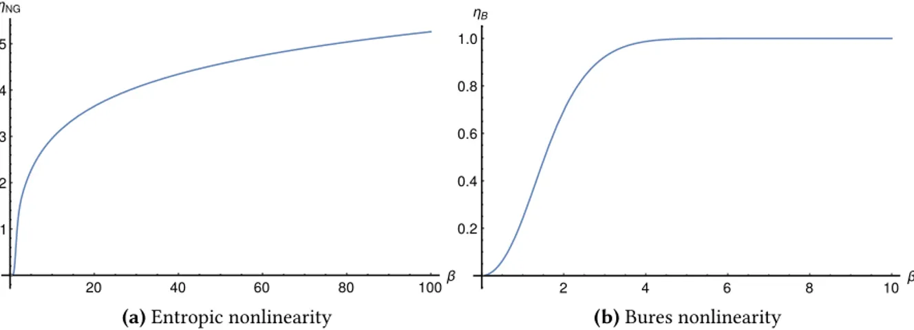
Despite being a very appealing quantity because of its interpretation, nonclassical depth is quite hard to compute in general and has a defect which makes it sometimes unsuited for practical purposes: it very often saturates to its maximum value 1. For example all number state have 𝜏_m = 1, despite of the number of photons. Actually if we restrict to pure states there is a quite general rule: it has been demonstrated [25] that the only pure states which have 𝜏_m < 1 are states with a Gaussian 𝑄 function, which are only the squeezed coherent states, defined as follows

|𝜉, 𝛽⟩ =𝐷(𝛽) ̂̂ _{𝑆(𝜉)|0⟩ = exp(𝛽 ̂𝑎}†− 𝛽∗_{𝑎) exp[}̂ 1 2(𝜉 ̂𝑎

†2_{− 𝜉}∗_𝑎2_̂

)]|0⟩; (1.66)

where ̂𝑆 is the so called squeezing operator. This fact poses a great limitation for the aim of the present work, since we will deal with pure states only and 𝜏_m would just tell us that the states are nonclassical, but not specify how much.

1.3.3 Negative Volume of the Wigner Function

Here we introduce a measure which will be very useful in the following chapters, which was proposed by Kenfack and Życzkowski [26]. As we stated previously the Wigner function is always a well behaved function, even if the 𝑃 function is singular, but it can attain negative values. Checking for negativities of the Wigner function has long been a practical way to witness nonclassicality in quantum optics, since it can be measured experimentally.

The intuitive idea is that measuring the volume of the negative part of this function can be used as a way to quantify nonclassicality. The following quantity 𝛿 represents the double of the volume of the negative part of the Wigner function

𝛿 = ∫d 2_{𝛼 [|𝑊 (𝛼)| − 𝑊 (𝛼)] =} (∫d 2_{𝛼 |𝑊 (𝛼)|} )− 1, (1.67)

where the equality follows from the normalization of the Wigner function and the integration is of course performed over the whole complex plane. A normalized version of this measure

(22)

can be defined in a straight-forward way:

𝜈 = 𝛿

1 + 𝛿, (1.68)

though in the following we will use 𝛿 rather than the normalized version, since there is no significant difference in their meaning. We can see that the calculation of this measure of nonclassicality boils down to the integration of the absolute value of the Wigner function, which is an achivable task (at least numerically) for a broader class of states than the previ-ous measures. The main disadvantage of this way of characterizing nonclassicality is that negativities in the Wigner function are just a sufficient condition of nonclassicality, since we can have a positive Wigner functions even for singular 𝑃 functions.

We also want to report that negativities in the Wigner function have been linked to other notions of nonclassicality, namely classical efficency in simulating a quantum system [27, 28].

A Remark About Nonclassicality of Pure States

If we concentrate just on pure states we have a theorem by Hudson [29] which affirms that the only states with a positive Wigner function are the squeezed coherent states (1.66). This is a quite relevant remark, because for the same class of states we have that the nonclassical depth is saturated to 𝜏_m = 1. So the complete picture is that for pure states these two measures are complementary, in the sense that when nonclassical depth becomes useless in distinguishing the quantity of nonclassicality, at the same time the measure 𝛿 become useful. The fact that 𝛿 ≠ 0 remains just a sufficient condition will still be a thing to keep in mind, because squeezing effects which do not change the volume of the negative part of 𝑊 can occur and not be captured by this measure.

1.3.4 Entanglement Potential

In quantum optics it has long been known that coherent states are the only states which produce uncorrelated outputs when going through a linear optics device [30], in particular nonclassicality has been identified as a prerequisite for having entangled states after a beam splitter [31]. From these considerations the idea of quantifying nonclassicality of a single mode state as the two mode entanglement at the output of a linear optic device was born, introduced by Asbóth et al.[32]. This measure is suitably called entanglement potential (𝐸𝑃 ) and it will be used extensively in the following analysis.

At first it seems that 𝐸𝑃 could be quite arbitrary, since in principle for any nonclassical state to be measured one would have to choose the auxiliary states and the optimal linear optics transformation to create as much entanglement as possible. It was shown in [32] that this is not the case and the optimal entangler is given just by a beam splitter with vacuum as an auxiliary state. This can be explained briefly by simple arguments.

Any passive linear optics transformation can be modelled by a generic circuit of beam splitters, see fig.1.1. We have one nonclassical input mode 𝜎 and a number of auxiliary states 𝜌_𝑛(ancillas). At the output we have an observer A receiving one output mode, an observer

(23)

Figure 1.1: (top) The general optical circuit for creating entanglement between A and B, 𝜌_𝑛are auxiliary clas-sical states. (bottom) The circuit can be simplified by choosing vacuum ancillas, the dashed box is local to B. Figure taken from [32].

B who gets a second mode and all the others outputs are measured by ideals photodetectors. The auxiliary input states must be coherent states, otherwise entanglement would not be caused just by 𝜎. A coherent state is just a displaced vacuum and displacing the auxiliary input states corresponds to the displacement of all the output states, in a way determined by the particular form of the circuit. Mixing the input modes states results in local mixing of the output states with additional classical communication. All these operations cannot increase entanglement, therefore we can choose |0⟩ as ancillas. With this choice the circuit can be recast in a simpler form, see fig.1.1, which is a single beam splitter splitting the input in two modes going to A and B, with the signal going to B split another arbitrary number of times. All measurements can be carried out using the modes of B, but local operations cannot increase entanglement, so there is no gain for B in splitting the beam and measuring just a part. This proves that the optimal entangler is a single beam splitter. The transmissivity of the beam splitter has yet to be choosen; even if there is no proof, it is argued in [32] that the 50:50 beam splitter is optimal independently of the input state.

As the last step we have to choose an appropriate measure for bipartite entanglement at the output; this is clearly a downside because different entanglement measures could lead to a different classification of nonclassical states. As long as we deal with a pure state 𝜌 in a finite dimensional Hilbert space the Von Neumann entropy of the reduced density matrix is a good measure of the entanglement of a generic state 𝜌 and it is defined as

𝐸[𝜌] = 𝑆[𝜌_𝐵] = − Tr_𝐵[𝜌_𝐵log 𝜌_𝐵]

= 𝑆[𝜌_𝐴] = − Tr_𝐴[𝜌_𝐴log 𝜌_𝐴], (1.69)

where 𝜌_𝐴 = Tr_𝐵𝜌 and 𝜌_𝐵 = Tr_𝐴𝜌 are the reduced density operators. In general they repre-sent completely different states but they always possess the same amount of Von Neumann

(24)

entropy, which, for a generic state density operator 𝜎, is defined as 𝑆[𝜎] = − Tr[𝜎 log 𝜎]. In the following we will deal with pure states so we choose to quantify entanglement with the measure 𝐸(𝜌). This choice corresponds to the entropic entanglement potential defined in [32], where entanglement is measured using the relative entropy of entanglement, which reduces to the Von Neumann entropy for pure states.

The evolution operator of the beam splitter has the following form

̂

𝑈 (𝜉) = exp{𝜉𝑎†𝑏 − 𝜉∗𝑎𝑏†} (1.70)

which can be disentangled using the Schwinger two-mode boson representation of SU(2) (see for example Ref. [33]) in order to achieve the normal ordering in the mode ̂𝑏:

̂

𝑈 (𝜉) = exp{−𝑒−i𝜃tan 𝜙 ̂𝑎 ̂𝑏†}(cos 𝜙)𝑎̂†𝑎− ̂𝑏̂ † ̂𝑏exp{𝑒i𝜃tan 𝜙 ̂𝑎† ̂𝑏} (1.71) where 𝜉 = 𝜙𝑒i𝜃_{. In this case ̂𝑏 is the mode associated with the vacuum input, so that ̂𝑏|0⟩ = 0}

and the operator exp{𝑒i𝜃_{tan 𝜙 ̂}_𝑎† _{̂𝑏} in (}_1.71_{) becomes the identity. To have a 50:50 beam}

splitter means choosing 𝜙 =𝜋

4; moreover we choose 𝜃 = 0 in order not to add a phase to the

output states. If we call ̂_{𝑈 (}𝜋

4) = ̂𝐵 then we can finally define the entanglement potential of

a generic state as

𝐸𝑃 [𝜌] = 𝐸[ ̂𝐵(𝜌 ⊗ |0⟩⟨0|) ̂𝐵†_]. (1.72)

1.3.5 Algebraic Measure

In a recent paper [34] a completely different approach to the problem of quantifying nonclas-sicality was proposed. This method is not related to quasiprobability distributions but it is based on the superposition principle. This is a fundamental feature of quantum mechanics and it is purely algebraic in nature, thus independent of geometrical features. For a pure sin-gle mode state this measure is defined as the minimum number 𝑟 of coherent states necessary to write it as follow |𝛹 ⟩ = 𝑟 ∑ 𝑖=1 𝜅_𝑖|𝛼_𝑖⟩. (1.73)

Since coherent states are the only pure classical states, this definition tries to capture non-classicality by counting how many classical states in superposition are needed to create the nonclassical state in exam.

The main feature of this measure is the fact that it can be used to quantify bipartite en-tanglement and nonclassicality in a unified way [35]. Exploiting the beam splitter duality between nonclassicality of the input state and entanglement of the output it can be proved that the minimum number of coherent states necessary to represent the input state is equal to the Schmidt rank of the output state. This results can also be extended to multimode states and multipartite entanglement.

This idea is conceptually very neat but it is in completely different from the other measures introduced and it gives a completely different hierarchy of states. For example it is known that the nonclassical depth of squeezed states is bounded from above by 𝜏_m = 1/2, while number states have 𝜏_m = 1; using this algebraic measure we have a completely different

(25)

result. It was shown in fact that 𝑟 = ∞ for squeezed states, while 𝑟 = 𝑛 + 1 for the Fock state |𝑛⟩. Another example is the famous cat state |𝛼⟩ + | − 𝛼⟩, which has negative parts in the Wigner function, therefore being more nonclassical than a squeezed state (with a Gaussian Wigner function); on the other hand according to this new definition the cat state has 𝑟 = 2 so it is minimally nonclassical.

We will not use this measure because it seems to capture a different notion of nonclas-sicality, giving such a different categorization. On a more practical level there is also an-other problem, which lies in the fact that 𝑟 is an natural number, so even if it quantitatively characterize some features correctly (number states with increasing 𝑛 are more and more nonclassical) it is unsuited to express a proper dependence on a continuous real parameter.

(26)

2 Quantifying the Nonlinearity of a

One-dimensional Potential

Oscillators are one of the most fundamental concepts in physics and they are used to repre-sent and model a plethora of different physical situations, both in the classical and quantum regime. The harmonic oscillator is the best known example and the easiest one to study, but nonlinear oscillators have attracted a lot of interest, both from a mathematical point of view and from a more applicative one.

In particular in the context of discrete variable quantum information nonlinear oscillators could be useful because they produce unequally spaced energy levels so they allow us to engineer two-level systems. On the other hand in continuous variable systems the concept of Gaussian states is fundamental, they are simply quantum states with a Gaussian Wigner function. Much of the efforts done so far in continuous variable quantum information in-volve this kind of states, even though in recent years non-Gaussian states have increasingly been recognized as an important resource for various quantum technology processes. In this context nonlinear oscillators could play an important role since their ground states and their equilibrium states are not Gaussian, as opposed to the ones of a quantum harmonic oscillator. These arguments are an indication that finding a method to quantify the nonlinear charac-ter of a quantum oscillator would be useful and incharac-teresting, since nonlinearity can represent a resource in various applications. One idea to do so could be to define a distance between potential functions and the reference harmonic potential, but this turns out to be not feasi-ble in general, since potentials do not need to be integrafeasi-ble functions. In this chapter we will present some ideas useful to quantify the the anharmonic character of a potential, by studying its ground state.

2.1 Quantifying Non-Gaussianity of a State

We now proceed to define a measure of the non-Gaussian character of a quantum state, as introduced by Genoni and Paris [36,37]. In doing so we will briefly review these ideas in a classical context and also review some properties of Gaussian states.

2.1.1 Classical Probability Distributions

In classical probability theory the Gaussian distribution is of paramount importance, thanks to the central limit theorem it is used to describe countless natural phenomena. Thus finding a way to quantify deviations from a perfect Gaussian behaviour is an important problem and

(27)

there are mainly two approaches. The former one is about evaluating the moments of the distribution, while the latter makes use of Shannon entropy.

The 𝑘th central moments of random variable 𝑥 with a probability density 𝑝(𝑥) are defined as 𝐸[(𝑥 − 𝜇)𝑘_{] =} ∫ ∞ −∞ d𝑥′_(𝑥′_{− 𝜇)}𝑘_𝑝(𝑥′_), _(2.1) where 𝜇 = ∫ ∞ −∞ d𝑥′_𝑥′_𝑝(𝑥′_). _(2.2)

The variable 𝑥 is Gaussian distributed if

𝑝(𝑥) = 1

√2𝜋𝜎2 exp{−

𝑥 − 𝜇

2𝜎2 }, (2.3)

where 𝜎2_{= 𝐸[(𝑥 − 𝜇)}2_{] is the variance.}

The first way to quantify non-Gaussianity is the kurtosis, defined as follows

𝐾(𝑥) = 𝐸[(𝑥 − 𝜇)4] − 3𝜎2. (2.4)

This quantity is zero for Gaussian variables and different from zero for most non-Gaussian variables, however it is not considered a robust measure since it may strongly depend on the observed data.

A more robust way to quantify non-Gaussianity is using the so-called differential entropy, which is the continuous version of the Shannon entropy and is defined as

𝐻(𝑥) = −

∫d𝑥

′_𝑝(𝑥′_{) ln 𝑝(𝑥}′_). _(2.5)

It is widely known that Gaussian variables are the ones that maximize this entropy at fixed variance, so this allows us to define a measure of non-Gaussianity called negentropy

𝑁(𝑥) = 𝐻(𝑔) − 𝐻(𝑥), (2.6)

where 𝑔 is a Gaussian variable with the same variance of 𝑥; negentropy is always non nega-tive and equal to zero only for Gaussian variables.

2.1.2 Quantum Gaussian States

Gaussian states are 𝑛 modes bosonic states with a Gaussian Wigner function, a general treat-ment of their properties is beyond our goals, but a complete review of the subject can be found in Ref. [33]. We will deal only with the simple case of a single mode state, so we just have a single pair of creation and destruction operators ̂𝑎 and ̂𝑎†_{, and a single pair of}

canonical operators ̂𝑞 and ̂𝑝.

Introducing the vector 𝑹 = ( ̂𝑥, ̂𝑝)𝑇 _{we can define the covariance matrix of a single mode}

states as follows

𝜎_𝑗𝑘 = 1

(28)

where { ̂𝐴, ̂𝐵} = 𝐴 ̂𝐵 + ̂̂ 𝐵 ̂𝐴 is the anticommutator. We also define the mean vector𝑿, its̄ components are 𝑋𝑘 = ⟨𝑅𝑘⟩.

A state is said to be Gaussian if its Wigner function is Gaussian and therefore can be written in the following manner

𝑊 (𝑿) = 1 2𝜋√det[𝜎]exp[− 1 2(𝑿 − ̄𝑿) 𝑇 𝜎−1 (𝑿 − ̄𝑿)], (2.8)

where 𝑿 = (Re 𝑧, Im 𝑧). This definition means that, even if Gaussian states are continuous variable states, they are the simplest ones because they are fully determined by the knowl-edge of ̄𝑿 and 𝝈. Gaussian states are in general generated by Hamiltonians at most bilinear in the mode operators, in particular the most general one mode Gaussian state can be written as

𝜌_𝐺 =𝐷(𝛼) ̂̂ 𝑆(𝜉)𝜈(𝑛) ̂𝑆†(𝜉) ̂𝐷†(𝛼), (2.9)

with 𝜈 being the single mode thermal state: 𝜈(𝑛) = (1 + 𝑛)−1_{[𝑛/(1 + 𝑛)]}𝑎†̂𝑎̂_{, where 𝑛 =}

Tr[ ̂𝑎†_{𝑎𝜈(𝑛)]. This statement is valid in general for states with more than one mode: every}̂ Gaussian state can always be written as an unitary transformation generated by an Hamilto-nian at most bilinear in the creation and destruction operators applied to a thermal state.

2.1.3 Distance From a Reference Gaussian State

Similarly to what has been shown in section1.3.1for nonclassicality one can quantify non-Gaussianity by measuring the distance from a reference Gaussian state. The reference state 𝜏 is a Gaussian state having the same first and second moments of the state 𝜌 in examination, that is to say

𝑿[𝜏] = 𝑿[𝜌]

𝜎[𝜏] = 𝜎[𝜌]. (2.10)

If we use the Hilbert-Schmidt distance 𝑑_HSin (1.60), we can define the degree of non-Gaussianity of a state 𝜌 as

𝑁𝐺_HS[𝜌] = 𝑑HS(𝜌, 𝜏)

𝜇[𝜌] , (2.11)

where 𝜇[𝜌] is the purity of the state defined as 𝜇[𝜌] = Tr[𝜌2

]. This measure can be thought as a quantum version of quantifying classical non-Gaussianity by using the moments of the distribution. It enjoys some properties (see [37] for more details): 𝑁𝐺_HSis equal to zero if and only if 𝜌 is Gaussian and it is invariant for unitary evolutions derived by Hamiltonians at most quadratical in the creation operators. Moreover this measure is proportional to the 𝐿2_{distance of the Wigner functions (or analogously the characteristic functions) of 𝜌 and 𝜏,}

this property can be written as 𝑁𝐺_HS[𝜌] ∝ ∫d 2_{𝛼 {𝑊 [𝜌](𝛼) − 𝑊 [𝜏](𝛼)}}2 𝑁𝐺_HS[𝜌] ∝ ∫d 2_{𝜆 {𝜒[𝜌](𝜆) − 𝜒[𝜏](𝜆)}}2 (2.12)

(29)

There is also a conjecture affirming that for single mode states the upper bound for 𝑁𝐺_HSis the value 1/2.

2.1.4 Entropic Measure

A different approach to measure non-Gaussianity is based on quantum relative entropy; for two quantum states it is defined as

𝑆(𝜌1‖𝜌2) = Tr[𝜌1(ln 𝜌1− ln 𝜌2)]. (2.13)

It can be proved that 0 ≤ 𝑆(𝜌1‖𝜌2) < ∞, when it is properly defined, which means that the

support of 𝜌₁is contained in the support of 𝜌₂_{. It has the important property that 𝑆(𝜌}₁_‖𝜌₂_{) =} 0 if and only if 𝜌₁ = 𝜌₂. While the relative entropy is not a proper metric, because it is not symmetric in its arguments, it has been used widely to quantify the distinguishability of two states. As a matter of fact the probability of confusing 𝜌₁with 𝜌₂after 𝑁 measurements for

𝑁 → ∞ becomes proportional to exp[−𝑁𝑆(𝜌1‖𝜌2)]

This leads to the definition of the entropic measure of non-Gaussianity

𝑁𝐺_E(𝜌) = 𝑆(𝜌‖𝜏), (2.14)

that is to say the quantum relative entropy between a state and the corresponding reference Gaussian state. This measure becomes

𝑁𝐺_E(𝜌) = Tr[𝜌 ln 𝜌] − Tr[𝜌 ln 𝜏] = 𝑆(𝜏) − 𝑆(𝜌), (2.15)

where 𝑆 denotes the standard von Neumann entropy and the equality follows because Tr[𝜏 ln 𝜏] = Tr[𝜌 ln 𝜏] for the way 𝜏 is defined. This measure can be considered as the quantum version of the negentropy (2.6) and it satisfies all the properties of the Hilbert-Schmidt measure plus some additional ones that will not be needed in the present work. However it is worth to mention that whereas the Bures measure is not additive under the tensor product operation, the entropic measure satisfies this property.

The von Neumann entropy of a single mode Gaussian state assumes a simple form

𝑆(𝜌_G_{) = ℎ(√det 𝝈),} (2.16)

where ℎ(𝑥) is a function defined as follows ℎ(𝑥) = (𝑥 + 1 2) ln(𝑥 + 1 2) − (𝑥 − 1 2) ln(𝑥 − 1 2). (2.17)

Thanks to this form the entropic non-Gaussianity becomes

𝑁𝐺_E_{(𝜌) = ℎ(√det 𝝈) − 𝑆(𝜌),} (2.18)

(30)

2.2 Nonlinearity of a Potential From Its Ground State

In order to measure the nonlinearity of a potential we are going to study its ground state [2]. In principle also the state at thermal equilibrium could be a good state to examine, but this makes computations more complex and it is yet to see if it is possible to work out such a measure explicitly for interesting cases.

The quantum harmonic oscillator has been partly reviewed in section1.1.1, in particular we have that its ground state wave function is a Gaussian:

𝜓_H_{(𝑥) = ⟨𝑥 ∣ 0⟩ = (}𝜔 𝜋 )

1 4

𝑒−12𝜔𝑥2, (2.19)

where the mass 𝑚 and the Planck constant have been rescaled to unity. We see that a har-monic oscillator is completely specified by the value of its frequency 𝜔.

On the other hand if we consider a generic potential 𝑉 (𝑥) which leads to an oscillatory behaviour the wave function can be obtained by solving the Schrödinger equation

[− 1 2

d2

d𝑥2 + 𝑉 (𝑥)_]𝜙(𝑥) = 𝐸𝜙(𝑥), (2.20)

which in general is not a Gaussian function. We denote by |0⟩_𝑉 the ground state of the system with the potential 𝑉 (𝑥).

Distance From the Ground State

The first idea to quantify nonlinearity relies again on the concept of geometrical distances between quantum states. In particular for this purpose the Bures metric (1.61) has been employed. If we denote the ground state of the reference harmonic oscillator by |0⟩_𝐻, the corresponding measure to quantify nonlinearity is defined as

𝜂_B[𝑉 ] = 𝑑_B_(|0⟩_𝑉, |0⟩_𝐻_), (2.21)

since the ground states are pure states this just reduces to

𝜂_B[𝑉 ] = √1 − |_𝐻⟨0 ∣ 0⟩_𝑉|. (2.22)

To have a proper definition we still have to choose a value for the frequency 𝜔 of the ref-erence harmonic oscillator, because the value of 𝜂B depends on it. The most natural choice

is expanding the potential near its minimum and finding 𝜔 as a function of the nonlinear pa-rameters of the potential, however determining this frequency is not always straight-forward and for some potentials it can even be misleading.

Nonlinearity Through Non-Gaussianity

We have stated that determining a reference harmonic potential might not always be possible so it would be useful to have a measure not dependent on the choice of a reference potential.

(31)

This is achieved by employing the entropic non-Gaussianity 𝑁𝐺_E, so that the measure of nonlinearity is defined as

𝜂_NG[𝑉 ] = 𝑁𝐺_E_(|0⟩_{𝑉 𝑉}_{⟨0|) = ℎ(√det 𝝈),} (2.23)

where the equality holds because the ground state is pure; 𝝈 represents the covariance matrix of the ground state.

This definition is more appealing than 𝜂_Bbecause it does not require the determination of a reference potential for 𝑉 (𝑥), but just a reference Gaussian state for the ground state of 𝑉 (𝑥). This renders 𝜂_NGindependent of the specific features of the potential, since we do not need to know the behaviour of 𝑉 (𝑥) near its minimum to computer the reference frequency.