Facoltà di Ingegneria Civile ed Industriale
DIAEE - Dipartimento di Ingegneria Astronautica Elettrica ed Energetica SIA - Scuola di Ingegneria Aerospaziale
Ph.D degree in “Energy and Environment”
AUTONOMOUS VEHICLE GUIDANCE IN
UNKNOWN ENVIRONMENTS
Candidate Supervisor
Marco Carpentiero Prof. Giovanni B. Palmerini
Index Of Contents
Introduction ... I
Chapter 1. Autonomous Guidance Exploiting Stereoscopic Vision ... 1
1.1 Introduction ... 1
1.2 Stereoscopic vision concept ... 3
1.3 The software architecture of the stereo-based navigation system ... 7
1.3.1 Stereo image acquisition ... 9
1.3.2 Stereo image processing ... 9
1.3.3 Obstacles Detection and Localization ... 13
1.4 Stereo Vision applied to robotic manipulators ... 14
Chapter 2. A Vehicle Prototype and its Guidance System ... 19
2.1 Introduction ... 19
2.2 The rover RAGNO ... 20
2.3 The guidance system ... 24
2.4 Test sessions ... 27
2.5 Conclusions and further developments ... 31
Chapter 3. Examples of Possible Missions and Applications ... 33
3.1 Introduction ... 33
3.2 Rover-Drone Coordination ... 38
3.2.1 Related works ... 38
3.2.2 RAGNO-UAV proposed architecture... 39
3.3 Experiment ... 41
Chapter 4. Guidance of Fleet of Autonomous Vehicles ... 47
4.1 Introduction ... 47
4.2 STAR: Swarm of Two Autonomous Rovers ... 49
4.3 Rovers’ implementation and trajectory choice ... 50
4.4 The guidance strategy ... 51
4.5 Simulations and results... 57
4.6 About the Navigation-Communications Subsystems’ Connection in Space Exploration Vehicles ... 59
4.7 Communication constraints ... 61
4.8 Planetary surface radio-propagation ... 62
4.9 Navigation ... 63
4.10 Estimation ... 66
Final remarks and future perspectives ... 69
I
Introduction
Gaining from significant advances in their performance granted by technological evolution, Autononous Vehicles are rapidly increasing the number of fields of applications. From operations in hostile, dangerous environments (military use in removing unexploded projectiles, survey of nuclear power and chemical industrial plants following accidents) to repetitive 24h tasks (border surveillance), from power-multipliers helping in production to less exotic commercial application in household activities (cleaning robots as consumer electronics products), the combination of autonomy and motion offers nowadays impressive options. In fact, an autonomous vehicle can be completed by a number of sensors, actuators, devices making it able to exploit a quite large number of tasks. However, in order to successfully attain these results, the vehicle should be capable to navigate its path in different, sometimes unknown environments. This is the goal of this dissertation to analyze and - mainly -to propose a suitable solution for this problem. The frame in which this research takes its steps is the activity carried on at the Guidance and Navigation Lab of Sapienza – Università di Roma, hosted at the School of Aerospace Engineering. Indeed, the solution proposed has an intrinsic, while not limiting, bias towards possible space applications, as it will become obvious in some of the following content. A second bias dictated by the Guidance and Navigation Lab activities is represented by the choice of a sample platform. In fact, it would be difficult to perform a meaningful study keeping it a very general level, independent on the characteristics of the targeted platform: it is easy to see from the rough list of applications cited above that these characteristics are extremely varied. The Lab hosted – before the beginning of this thesis activity – a simple, home-designed and manufactured model of a small, yet performing enough autonomous vehicle, called RAGNO (standing for Rover for Autonomous Guidance Navigation and Observation): it was an obvious choice to select that rover as the reference platform to identify solutions for guidance, and to use it, cooperating to its
II
improvement, for the test activities which should be considered as mandatory in this kind of thesis work to validate the suggested approaches.
This dissertation has been conceived as a focused, detailed description of the results achieved during the period as PhD candidate. It is not intended to offer a global view of the Guidance and Navigation subsystem applicable to autonomous vehicles, that should encompass many more different techniques and algorithms specialized for the different applications. Instead, it has been preferred the studies and findings authored during the period. Such a choice has been due to both (1) the opinion that the global scenario description would have required a really remarkable experience (especially a “hands-on” one to appreciate effective advantages and disadvantages of the past, existing or designed) still unavailable at the PhD level, and indeed (2) the risk to produce a kind of (almost useless) repletion of surveys already available in literature without addition of any significant contribution.
On the other side, the approach selected allowed to duly discuss the peculiarities of the problems tackled during the research and of the proposed – and tested – solutions, indeed at least attempting to offer a maybe useful and certainly original contribution. The present dissertation has been divided in four main chapters, each of them focused on a relevant topic of the research.
Chapter 1 deals with the main topic of the work, i.e the stereoscopic vision applied for autonomous guidance problem. The concept and theory of the stereovision are presented in detail together with its application in the field of computer vision such as the image processing. The most important features descriptors (BRISK and SURF) are then analyzed to prove, even with experimental results, their effectiveness for objects recognition and localization scope. The last part of the chapter reports an example of application of the stereovision system in the field of the robotics manipulation as it spread from industrial plant (e.g. pick and place machines) to space applications (e.g. on-orbit servicing, visual inspection and so on).
III
Chapter 2 presents the wheeled rover, RAGNO, involved in the various test sessions to demonstrate both the efficiency and the limits of the implemented guidance algorithms based on the stereovision principles. The first part of the chapter is dedicated to the hardware architecture of the rover focusing on the modular concept adopted during the design and realization phases. In the second part of the chapter the attention moves on the description of the implemented and tested guidance algorithms: the Lyapunov-based strategy and the A-star graph-Lyapunov-based guidance law.
The former is a well-known solution adopted for the guidance problem (especially in space applications like probes descent phase and landing) while the latter represents a milestone of the current work since it has been designed and developed during the research period. The results of simulation and tests are reported to demonstrate the advantages, of the A-Star approach with respect to the classic one both from the analytical and computational point of view.
Chapter 3 deals with the experimental campaigns lead by involving RAGNO in a stand-alone or cooperative formation. In addition, the needing of communication rules between members of swarm or formation of autonomous robots has been introduced. Chapter 4 describes a possible architecture for the guidance of a fleet of autonomous robots operating in an unknown scenario with different tasks, considering the results and limits discussed in the previous chapters. In the first part of the chapter, the STAR (Swarm of Two Autonomous Rovers) rovers configuration is proposed as a possible swarm architecture for planetary exploration. The A-Star guidance algorithm has been adopted and a first attempt of communication protocol has been developed to ensure a coordinated and safe ground exploration and mapping. Simulation results are reported to prove the feasibility of the selected approach and its limits. The second part of the chapter focuses on the intra-platforms communication that is surely the main topic in the case of swarm exploration. The characteristics and constraints of the link, due to the disturbances that affect the planetary surface radio propagation, are analytically
IV
presented. Finally, the last part of the chapter deals with the navigation system architecture designed for the STAR mission with the description Kalman algorithm needed for kinematic state estimation.
1
Chapter 1.
Autonomous Guidance Exploiting Stereoscopic Vision
1.1 Introduction
Computer vision attained extremely significant advances in recent years, thanks to continuing development of sensors, software and powerful computation resources [1]. Indeed, the applications spread in different areas, and especially in the ones closer to state-of-the-art technology. Among them, space engineering is clearly an elective area, and the Mars exploration carried out by planetary rovers is a very remarkable example for this technology [2].
Future space missions are likely to continue in exploiting computer vision systems, which are able to provide high accuracy and a rich and comprehensive autonomous perception of the scenarios/environment. Aside from the topic of the rover navigation, spacecraft proximity manoeuvres and in-orbit servicing also offer a wide area for possible applications. Until now, main tasks of computer vision in this field have been the detection and recognition of objects whose shape is already known: this approach was adopted in the automatic rendezvous, carried on by identifying specific markers in acquired images [3]. The improvements in optical sensors' quality, software skills and computational power allow today to attempt a full reconstruction of the observed scene, practically in real time. The capability to detect and avoid obstacles opens the possibility of robotic autonomous operations in the difficult, unprepared scenarios of orbital operations, where visual guidance of the manipulators would be extremely effective [4]. If in-orbit operations already present stricter requirements with respect to planetary rovers in terms of the guidance-navigation-control loop bandwidth, there are landing and very low altitude flights over unexplored, unknown landscapes that will be the ultimate, not yet fully attained goals.
Independently of the application, the performance of autonomous computer vision systems depends on the sensors adopted to gather data, on the software to exploit them,
2
and on the computation hardware to run these complex codes. With reference to the visual sensor, a classical partition differentiates active instruments (LIDAR, time-of-flight cameras) from passive ones, bounded to make use of external light. Aside from the source of the radiation, a very important asset of active sensors is their capability to detect the evaluate the depth in the captured image, allowing for a 3-D vision. Such an advantage is usually paid in terms of cost and complexity, in addition to mass/volume/power requirements which are sometimes difficult to match with the characteristics of spacecraft. It is not the case of simple, monocular passive viewer, which are instead limited to a 2-D representation. Stereoscopic vision, by combining two images captured from different points of view, has the capabilities to provide information about the depth without increasing too much (or even at all) the issues about sensors. On the other way, a large role is left to the data processing, as the features appearing in the two images captured at the same time need to be identified and coupled in order to provide 3D measurements. However, such a significant limit becomes less rigid in view of the continuing advances (both hardware and software) in computer science.
It is reasonable to claim that stereoscopic vision will have an important role among computer vision techniques for space applications. Impressive advances in real time processing of the image pairs are expected, also – and above all – driven by terrestrial automotive market. As a result, overall architecture advantages of the stereo viewer with respect to other 3D capable solutions are deemed to dominate, especially for small spacecraft (either small rovers or satellites equipped with manipulators).
Indeed, this chapter is aimed to discuss possible applications of the stereoscopic vision. Next paragraph will recall main concepts for this technique. Then, some remarks about use of stereo-vision in manoeuvring space manipulators are presented. Later, considerations on stereo-vision applied to the navigation of a vehicle are reported. Finally, a real-world example is detailed, referring to the small rover RAGNO which main characteristics will be reported in next chapter. The solution for the
guidance-3
navigation-control loop of this rover, based on a stereo viewer accommodated on board and able to detect obstacles and compute a path avoiding them is presented. Quantitative data from numerical simulations and from road tests are reported, with the aim to show – even within the limited scope of a lab project – the main characteristics of a stereo-vision system.
1.2 Stereoscopic vision concept
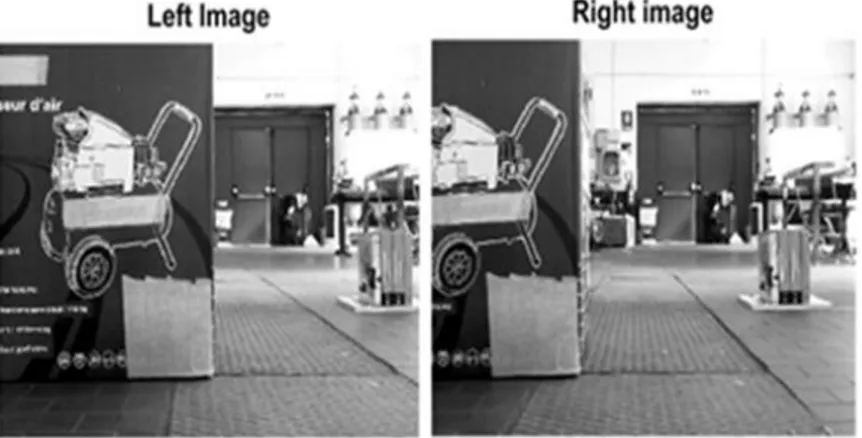
An ideal stereoscopic viewer is composed of two identical cameras with parallel optical axes (Figure 1-1). This set-up allows to observe the scene from two points of view and to compute the optical depth of a detected point of the scene (P) by means of a simple triangulation between P and its projections on the right- (PR) and the left-camera (PL) image planes. PL and PR (which identification in the images and association with P is for now assumed) are also defined as corresponding points.
Once selected a reference frame rigid to the left camera, it is possible to express the triangulation relations considering both cameras like pinholes [5]. For a pinhole camera (Figure 1-2) the relation between a point P belonging to the scene and the relevant image point PL can be found through the similarity criterion for triangles, stating that two triangles are similar if they have two proportional sides and the angle between these sides equal.
4
Figure 1-2: Pinhole camera and similar triangles; X, Y, Z are the coordinates of the captured point P in a frame centered in the camera, u, v the corresponding coordinates of its projection in the image
plane.
Applying this similarity criterion to the ⊿(CKH)-⊿(COH’) and ⊿(CHP)-⊿(CH’P’) pairs of triangles it is possible to write:
u v X u = f + p Z Y v = f + p Z
Eq. 1-1: Image coordinates of point P
Eq. 1-1 can be rewritten in matrix form by means of homogeneous coordinates:
u L v u X f 0 p Z P = Z v = K P = 0 f p Y 0 0 1 1 Z
Eq. 1-2: Homogeneous coordinates of point P
Eq. 1-2 is also labelled perspective law because it projects the point P from the reference frame characteristic to the scenario to the image reference frame. The K matrix is defined as the intrinsic matrix of the camera and its elements can be determined through a calibration procedure [6].
The perspective law (Eq. 1-2) includes two equations with three unknowns (X, Y, Z), thus resulting unsolvable. This is the reason why it needs a second camera to obtain the optical depth of the point P. The application of the perspective law to the stereo viewer leads to the following relations:
5 L L L T T R R R R Z P = K P Z P = K R (P - C )
Eq. 1-3: perspective law in left-camera frame
where R and C matrices take into account the relative position and orientation of the second camera. In the ideal case sketched in Figure 1-1, with the baseline between the cameras orthogonal to the optical axes, which are parallel, and a similar arrangement for image planes and resolution, it follows that the intrinsic matrices are equal and that the rotation matrix corresponds to the identity.
Indeed Eq. 1-3 becomes:
L T R R Z P = K P Z P = K (P - C ) to be expanded as: L u L v R u R v X Y u = f + p v = f + p Z Z X-b Y u = f + p v = f + p Z Z
Eq. 1-4: Pixel coordinates of point P in left and right camera image plane
Since cameras are supposed identical, the second and fourth equations of Eq. 1-4 can be neglected. By subtracting the first and the third it is finally possible to obtain the third dimension, i.e. the optical depth Z,
L R f b f b
Z = =
u - u d
Eq. 1-5: Optical depth Z
which evaluation depends on the focal length, on the relative geometry between the cameras and on the parameter d called pixel disparity: the closer the scene point P, the higher the disparity.
6
Figure 1-4 shows an example of pixel disparity (disparity map) for the sample scenario depicted in Figure 1-3Figure 1-3, where there are two objects at different distances from the stereo viewer.
Figure 1-3: A sample of stereo images
Figure 1-4: Disparity map for the scenario depicted in Figure 1-3
According to Eq. 1-5, it can be seen how the foreground box is characterized by a greater pixel disparity than the background objects. However, the raw disparity map shown in Figure 4 does not allow to detect the obstacles easily. In fact, there are many sparse color spots, for example those corresponding to the floor, which do not identify an existing obstacle. Therefore, a cleaning algorithm should be implemented to filter out this noise and to identify the true obstacles. This process could require a high computational time because the disparity map should be analyzed pixel by pixel. So, another approach – based on the object recognition techniques - has been chosen in this work in order to save the computational time.
7
1.3 The software architecture of the stereo-based navigation system
The architecture of the navigation software developed for obstacles detection and localization consists of three blocks:
stereo image acquisition
stereo image processing
obstacles detection and localization in the (X, Z) motion plane
The resolution of the Eq. 1-5 requires the knowledge of the viewer’s baseline and of the cameras focal length. The former is a geometric parameter and it can be chosen by the user while the latter is an intrinsic characteristic and it must be determined through a calibration procedure. The Zhang’s method [6] has been adopted for the calibration of the stereo-viewer. This method allows to determine the intrinsic parameters of both cameras and their relative orientation by solving the perspective law for a set of points called markers. These markers belong to a predefined 2D calibration object and their (X, Y, Z) coordinates are known. The most used calibration object is a rectangular chessboard with squared cells of known dimensions (Figure 1-5).
Figure 1-5: The calibrator object and the sample marker
The markers are identified in the vertices of each cell. By writing Eq. 1-2 in a reference frame rigid to the chessboard, the cameras orientation (R) and position (t) with respect to this frame must be taken into account:
T T T T T i h h
P
P = λ K R (P - ) = λ K R | -R
= λ K R | -R
P = H P
1
t
t
t
8
H is a rectangular matrix (3x4) and is called homography. It is possible to make H square by taking into account those markers having the same Z coordinate which can be set to zero without loss of generality. In this way, the previous equation reduces to the following:
T i 1 2 3 1 2 1 2 3 h X u X X Y P = v = λK r r r -R t = λK r r t' Y = h h h Y = H P 0 1 1 1 1 The Zhang’s method allows to determine the stereo parameters by calculating the homography H through the knowledge of a set of (Pi, Ph) points pairs. In order to obtain an accurate calibration of the three axes of each camera it needs to acquire chessboard’s images from different points of view. The results of Zhang’s calibration procedure are the following: L R 605.9893±1.1312 0 331.9116±0.5466 K = 0 605.2356±1.1355 238.8710±0.6377 pixel 0 0 1 603.0425±1.0914 0 316.9373±0.7559 K = 0 602.4318±1.0880 231.9409±0.5975 pixel 0 0 1 L R 0.9992 0.0066 -0.0397 R = -0.0066 1 0.0015 0 0397 -0.0015 0.9992 . t = 148.5633 4.7982 4.6790 mm
The above results show that the principal points (i.e. the center of projection) of the webcams do not correspond with the center of the respective CCD sensor. The values of the rotation matrix and the translation vector are almost similar to the expected ones. In fact, the stereo viewer has been built with a baseline of 15 cm while the two cameras are aligned along the X axis.
9 1.3.1 Stereo image acquisition
The built in Matlab® USB webcam package allows the user to define the webcam object and to set its properties like the image resolution and the value of the focus. For the stereo viewer used, the standard resolution 640x480 and the autofocus mode have been chosen. The acquisition of the stereo image generates two 3D matrices which dimensions are 480x640x3. The third dimension refers to the number of colors used to define the single image i.e. the RGB three-color. Each element of the image matrix is defined as an 8-bit integer, so it assumes a value in the [0-255] range. As the processing phase requires a greyscale image, the following conversion is needed:
I = 0.2989 R + 0.5870 G + 0.1140 B
1.3.2 Stereo image processing
The resolution of the triangulation problem Eq. 1-5 assumes a previous knowledge of the corresponding points’ coordinates (PL, PR). The identification and matching of these points’ pairs represents the main and most computationally expensive step of the whole navigation algorithm, since it needs a significant stereo image processing. In recent years, thanks to the constant improvement in computing power and software skills, several matching techniques have been developed with the goal to reduce the required computational time and to improve the robustness of the algorithms.
The typical process can be divided into two different phases:
research, extraction and characterization of particular points, called features, in both images
comparison of left and right extracted features and matching of the corresponding pairs
A feature can be defined as a small region of the image characterized by one or more repeatable properties. There are different types of features depending on the researched properties:
10
edge: it is a point of the image characterized by a discontinuity in the brightness gradient. This feature allows to identify the edges of a scene’s object
corner: it is a point identified by the intersection of two edges where the gradient has a significant curvature. This feature allows to identify the corner of a scene’s object
blob: it is a region of the image characterized by peculiar properties (e.g. brightness) with respect to the surrounding area.
Every kind of feature can be extracted by means of different detection algorithms, while each extracted point needs to be coupled to a descriptor vector with these properties:
distinguishability: the descriptor has to make the generic feature distinguishable from the others. The level of distinguishability depends on the dimension of the descriptor
robustness: the descriptor must be detectable in any lighting conditions and regardless of photometric distortions or noise
The choice of the descriptor depends on the goal of the image processing. For the purpose of obstacles identification, it needs a combination of detector-descriptor which does not require high computational time. After an accurate analysis of the existent extraction algorithms, the SURF (Speeded Up Robust Feature) and BRISK (Binary Robust Scale Invariant) detectors have been chosen.
SURF [15] is a blob detector with an associated descriptor of 64 elements. The detection algorithm is a speeded-up version of the classic SIFT detector. The generic feature is extracted by analyzing the image in the scale space and by applying sequential box filters of variable dimension. The features are then localized in the point of the image where the determinant of the Hessian matrix H(x,y) is maximum. The descriptor vector is than determined by calculating the Haar wavelet [19] response in a sampling pattern centered in the feature.
11
BRISK [16] is a corner detector with an associated binary descriptor of 512 bit. The generic feature is identified as the brightest point in a sampling circular area of N pixels while the descriptor vector is calculated by computing the brightness gradient of each of the N(N-1)/2 pairs of sampling points.
Once left and right features have been extracted, their descriptors are compared in order to determine the corresponding points pairs. The matching criterion consists in seeking for the two descriptors for which their relative distance is minimum. This distance corresponds to the Euclidean norm for SURF case and to the Hamming distance for the BRISK one. The latter distance is intended as the minimum number of substitutions needed to make two binary strings equal. The matching process seems to require a very high computational time because each left feature should be compared with all right ones. This may be true for object recognition processes where the algorithm has to identify a particular object by comparing its acquired image with a database of images. Instead, in the case of stereovision applied for obstacles detection, the computational time can be reduced by taking into account the theory of the epipolar geometry. In fact, it states that there exists a geometric constrain between the left and right projection of the scene point P. As a consequence, the space where a matching feature has to be researched reduces to a portion of the image.
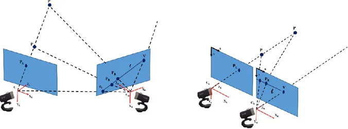
Figure 1-6: Epipolar geometry for real and ideal stereo viewer (in the ideal setup the epipolar point is at infinity because the sheaf of epipolar lines is non-regular. lines are in fact parallel).
12
As shown in Figure 1-6, for a fixed PL the corresponding PR lies on the line l, called epipolar, whose inclination depends on the geometry of the viewer. The position of PR varies depending on the depth of the scene point P. In the case of a real stereo viewer, the epipolar line is delimited by the epipole point e1 and the vanishing point V. The first is
the center of the regular sheaf of epipolar lines and corresponds to the projection of CL on the right image plane while the second is the projection of a scene point P with infinite depth. For the ideal stereo viewer used, the epipolar lines are horizontal therefore two matching features will have roughly the same v-coordinate. The searching process can be limited to a subset of right image rows thus obtaining a time savings.
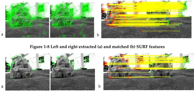
Figure 1-8 and Figure 1-9 show the results of the processing phase for the sample space-like scenario in Figure 1-7. The irregular shape together with the color non-homogeneity of the close object entail that more SURF features than BRISK have been detected. By comparing the results obtained with features extraction to those of disparity map, it can be note that the former does not require a post processing noise filtering because there are few outliers which can be cut out by mean of a selection operation. On the contrary, the obtained disparity map shows the obstacle shape very well but a lot of noisy values too. A post processing filtering is therefore mandatory in order to make the map easily exploitable.
13
Figure 1-8 Left and right extracted (a) and matched (b) SURF features
Figure 1-9 Left and right extracted (a) and matched (b) BRISK features
Regarding the computational effort, the results are summarized in Table 1-1 and Table 1-2. The onboard computer is a quadcore PC with a 2.4 GHz CPU and 8 GB RAM.
Extracted (L/R) Matched
BRISK 236/200 65
SURF 526/496 216
Table 1-1. Extracted and matched features
Detection Matching Total
BRISK 238 79 317
SURF 141 79 220
Table 1-2. Computational time of detection and matching process (in ms)
1.3.3 Obstacles Detection and Localization
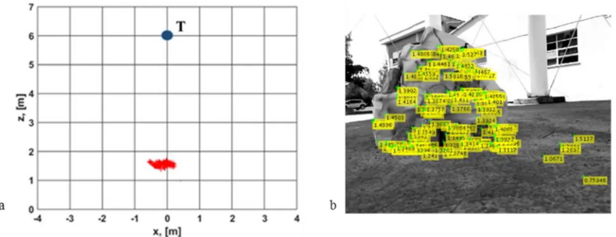
Once the viewer has been calibrated and the correspondences have been found, the triangulation equation Eq. 1-5 can be solved. As the mission is supposed in a 2D space, the triangulation results are reported in the (X,Z) rover reference frame. This frame has the same axes of the camera reference (but it is applied in the vehicle center of gravity. In order to select only the most interesting points among the set of triangulated ones, a threshold value is imposed on the optical depth Z. All the points with Z > 2m have been cut out thus saving only the foreground features. The criterion adopted for obstacles
14
identification is based on the evaluation of the features density. The (X,Z) plane is divided into square cells for each of which the density of contained features is calculated. A threshold value dTH is then established. All the cells with a density greater
than dTH is marked as occupied by an obstacle. The threshold value depends on the
discretization step: the higher it is and the lower the threshold has to be. Figure 1-10 shows the result of selection and identification process: background features have been cut out together with the low density ones.
Figure 1-10: Obstacle localization in 50cm step discretized (X,Z) plane (left) and depth marks in camera image (right)
1.4 Stereo Vision applied to robotic manipulators
The goal to identify the information about depth is important in every scenario, including for sure the operational domain of a robotic manipulator. The application of stereovision to this specific field has been already considered as mature [7] for terrestrial, secluded environments, as the one typical to pick-and-place machines. In the industrial field the interest for stereoscopic vision deals with the limited costs and the reasonable complexity of the system. In fact, off-the-shelf imaging devices and easily designed software with standard hardware can successfully attain good performance. A totally different assumption should be done with respect to space applications, as manipulation of captured/grasped spacecraft for in- situ servicing. These applications, while deeply in need of a 3-D vision system, have nevertheless two important, limiting characteristics:
15
the scenario is not repetitive at all;
the light conditions change (even suddenly) in time, due to occlusions occurring during the manoeuvre.
These two characteristics deeply affect the peculiar advantage of the stereo-vision systems as implemented in manufacturing industry today. However, the comparable active systems capable to intrinsically solve the 3-D issue, as LIDAR or time of flight cameras, turn out to be extremely expensive. Moreover, they can have significant limitations in terms of power/mass/volume requirements or in terms of performance, especially as far as it concerns the maximum attainable distance. As a result, stereoscopic vision, as a passive technique where much effort is left to the software/computation side (i.e. to an extremely fast advancing area) has a large interest also for space applications. Even more, it is maybe the only suitable solution for small platforms (Figure 1-11).
Figure 1-11: A sketch of a possible stereo-vision system accommodated on a small satellite help in-orbit servicing. The Sun recalls about sudden switches from shadow to full light conditions which affect image analysis.
The identification of the different features in the pictures captured by the two cameras to provide meaningful pairs (uL, uR) and (vL, vR) in Eq. 1-4 becomes a consuming task (these techniques will be discussed in the following of the thesis). In fact, the two recalled limits associated with the generic applications in space require a careful analysis of the two images, making use of advanced artificial intelligence tools. To ease such a process, it can be noticed that the positioning of the robotic arms’ elements in the
16
scenario can be actually computed by using markers purposely located at the joints (Figure 1-12, [8], [9][10]).
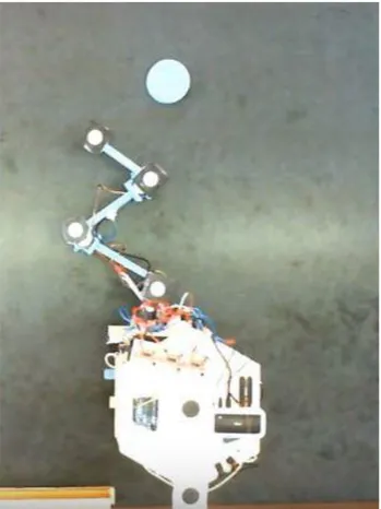
Once the arms’ configuration and the other features of interest, as the target in Figure 1-12 sketch, have been identified, the computation of the relevant coordinates can be carried out by means of the process expressed by Eqs.(1)-(6). Likely, the final goal for these applications is the evaluation of the commands to be given to the arms in order to execute the required operations. An interesting, complete example for such a task has been reported, even if in simpler laboratory scenario, in [9][10]. The idea is to draw on the images, by means of a geometrical approach, a reference frame which will provide the relative coordinates of the target with respect to the manipulator elements. This drawing obviously takes into account the fact that depth can be computed by stereoscopic technique only by comparing the images from two cameras. Then, the computed relative state of the elements allow to command the torques to be provided by the motors at the arms’ joints.
17
Figure 1-13: A sketch of the geometrical approach to draw a reference system to enable the computation of the distance to the target and the relevant commands for the manipulator. The drawing is performed in each single image to later reconstruct the 3D scene by comparison between two cameras [9][10]. Links of the manipulator are represented as dashed lines as they are actually projections, lacking the third dimension, and therefore not in scale with the real elements
Aside from the arrangement depicted in Figure 1-11, there is the opportunity to exploit the capability to accommodate the cameras on the arms of the manipulator. This solution has been recently proposed in a test to accurately compute the kinematics of the arms [11], practically offering a back-up of the encoders. Such a configuration, in spite of the possible need for an iteration of the calibration process, can offer distinctive advantages, as it allows to better capture close scenarios, being also more robust to occlusions. Basically, this arrangement generates a shift from the classical hand-in-the-eye configuration to the more flexible hand-in-the-eye-in-the-hand one [12], that turns out to be convenient in some specific operation. Furthermore, standing the typical length of the links of the space robotic arms, this arrangement can offer a significant increase in the baseline between a camera located on the bus and the other located at the end effector. In such a case, previous relation Eq. 1-3 should be modified as
{
Z P
L= K
LP
Z P
R= K
R(P-C
∗RT)
18
where the intrinsic matrices of the camera (K) become different as different could be their focal length, and the vector C* can easily have all elements different from zero. In fact, the angle β in Fig. 8 is not constrained to be equal to 90° as in typical applications (and in human vision) where the optical axis is orthogonal to the baseline.
According to Eq. 1-5, the increase in baseline grants a high disparity for the same focal length and optical depth, or – in other words - an extension of the maximum suitable range for a given resolution of the camera sensor. Such an advantage ca be extremely important when dealing with proximity navigation [13], i.e. in the preliminary phases of the rendezvous leading to in-orbit servicing manoeuvres (Figure 1-14).
Figure 1-14: A sketch of the geometrical approach to enable the computation of the distance to the target and the relevant commands for the manipulator
Finally, we can claim that computer vision techniques are expected to be the workhorse of future autonomous space missions. Among them, stereoscopic vision is considered a very interesting option, as requirements easily fit the volume, mass, power limitations of typical space vehicles. An outline of the stereoscopic vision technique has been presented, with likewise applications in the fields of the space manipulators and of the planetary exploration. Specifically, the case of a rover has been carried out in detail, including the design of the vision-based navigation system, its implementation on board a small terrestrial autonomous vehicle, and the test campaign.
19
Chapter 2.
A Vehicle Prototype and its Guidance System
2.1 Introduction
Planetary exploration through mobile laboratory platforms has always been one of the most important topic of space engineering. The first examples are the American lunar vehicles and the Russian remotely control Lunokhod 1-2. Since the early 90s the space agencies focus on the exploration of Mars. NASA was the first to land a platform on the Red planet with the Sojourner (1996, Mars Path Finder). Till today other three rovers have landed on Mars: Spirit and Opportunity (2004, Mars Exploration Rover) and Curiosity (2011, Mars Science Laboratory). These platforms are the unique examples of autonomous mobile robots designed for planetary exploration. Autonomy has been accomplished by integrating a panoramic binocular vision system (NavCams). NavCams1 software is able to identify and localize close obstacles by processing the acquired stereo image. This navigation system has been improved in Curiosity, where other four stereo pairs (Hazard avoidance cams) has been added in order to obtain a wider vision of the surrounding environment. Future Mars platforms like NASA’s Mars 2020 and ESA’s ExoMars 2018 are going to integrate a further improvement of the stereo-based navigation system. The reasons of the great success of the stereoscopic vision are multiple. At first, stereo vision is an attractive technology for rover navigation because is passive, i.e. sunlight provides all the energy needed for daylight operations. The second reason is that only a small amount of power is required as for the cameras electronics as to obtain knowledge about the environment. In addition, by installing enough cameras or cameras with a wide field of view, no moving parts are required to capture the 360° surrounding environment. Having fewer motors reduces the number of components that could fail. Thanks to the constant improvements in computer vision techniques, hardware performances and optical sensors quality, future space missions
20
are likely to exploit stereo-based systems for applications aside from the rover navigation. Typical examples are the proximity maneuvers, like rendez-vous or docking, but also the more general in-orbit servicing like autonomous robotics arm grasping and manipulation of objects with unknown shapes.
This chapter deals with the application of the stereoscopic vision to rover navigation in order to make the platform totally autonomous. The design and development phases are explained in details together with the results obtained during a test session. In particular, Section 2.2 introduces the rover RAGNO used in his work: its starting and current state of the art is described in details. Section 2.3 is focused on the guidance strategy needed to plan a safe path leading the rover toward the final goal position. Section 2.4 shows the results obtained during the test campaign while the last Section 2.5 summarizes the main points of this work and suggests future applications of both autonomous vehicles and stereovision.
2.2 The rover RAGNO
RAGNO [28], standing for Rover for Autonomous Ground Observation and Navigation, is a four wheels small rover originally designed in 2011 at the Guidance and Navigation Lab, Sapienza Università di Roma in order to familiarize with robotics platforms, multibody systems and remote control. RAGNO can be defined as a modular vehicle because different subsystems, for example a robotic arm, can be allocated onboard according to the mission needs.
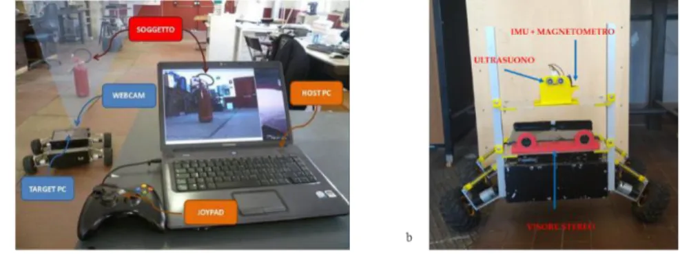
In the present project RAGNO has been equipped with a stereo viewer and a sensors platform containing a triaxial gyroscope and a triaxial magnetometer. This hardware integration allows to convert the rover from a remote-control system (Figure 2-1a) to an autonomous one (Figure 2-1b). The reading of sensors measures and the control of the angular velocity of the four wheels are realized by two Arduino shields. All the data are then sent to the guidance and navigation Matlab software through a serial communication.
21
Figure 2-1: Initial (a) and final (b) RAGNO state of the art RAGNO
The rover RAGNO (Rover for Autonomous Guidance Navigation and Observation) developed at the Guidance and Navigation Lab of the University of Rome, “La Sapienza”, is a friendly multi-task mobile platform. RAGNO has been used in different studies concerning the remote control (Figure 2-2, left), the multibody dynamics when equipped with a robotic arm (Figure 2-2, right) and the operational autonomy through stereo-based navigation [14], which is the focus of this section.
Figure 2-2: Applications of the RAGNO rover
For such an application, with the goal to reach a target while avoiding the obstacles in the scene, RAGNO is equipped with a commercial stereo viewer, a three axes magnetometer, a gyroscope and a central processing unit (Figure 2-3). The stereo viewer is essential to understand a 3D scenario and autonomously detect and localize the obstacles to define an optimum and safe path towards the target. Notice that the stereo viewer requires a calibration [6] before the mission begins to attain the desired accuracy. The gyro and the magnetometer are instead needed for the control section to reconstruct RAGNO true path by means of a Kálmán filter implementation. The comparison
22
between the desired and the Kálmán estimated paths generates the commands for the four-wheels motors to correct tracking errors by applying a speed control law.
Figure 2-3: The RAGNO rover as equipped for the project
Figure 2-4: Sample outdoor scenario
Figure 2-5: The location of the obstacle resulting from the use of the stereo vision system is depicted in a map to help the identification of a convenient path from the current position (0,0) to the target T.
23
By applying Eq. 1-5 to matched points’ pairs it is possible to obtain the 2D map (of the plane containing the rover motion) depicted in Figure 2-5. In order to plan a safe path toward the target position T, a guidance law needs to be implemented. A suitable solution is represented by a graph-based guidance law [14], which allows the rover to reach the target moving on the shortest path. However, tracking errors easily occur while following this desired optimal path. By means of the additional sensors (gyro and magnetometer) it is possible to feed with relevant measurements a Kálmán filter built on a simple dynamic model, and to obtain an accurate estimate of the actual path. At this stage, the control section commands the wheel motors to ensure the tracking of the correct path.
Figure 2-6: Planned and Kálmán estimated path
The findings from path planning and tracking tasks are shown in Figure 2-6 above: the black line indicates the desired path while the red one the estimate of the actual trajectory. The guidance algorithm requires about 400 ms to compute the shortest path, while the whole guidance and navigation algorithm time requests is in the order of 1 s, a value deemed satisfactory for a space rover moving at limited speed in a static environment.
24 2.3 The guidance system
The output of the navigation system, i.e. the coordinates of the localized obstacles, becomes one of the inputs of the guidance system. The purpose of the designed guidance algorithm is to plan a safe path that brings the rover from its starting position toward the target. Different guidance strategies can be found in literature [27]. One of the most used solutions in space-related problems like rendez-vous, descent and landing is based on the Lyapunov’s stability theory. This approach provides to define a custom function, the artificial potential V, which describes the interaction between the body and the surrounding environment. The motion of the RAGNO platform can be compared to a sample positive charged particle in an electric field generated by other particles: the sample particle is attracted by the negative (the target) and repulsed by the positives (the obstacles). In the electric analogy, the total action exerted by the charges is the Coulomb’s force and it corresponds to the gradient of the potential function V. For the purpose of rover path planning, as the problem is kinematic, the following potential function of the platform velocity has been elaborated:
2 bs
2 2
att rep t t obs,j 0
j =1 obs,j 0 2 att #o t obs,j 0 1 1 1 1 V +V + η - 2 2 V = 1 V > 2
Eq. 2-1: Expression of the potential function
The potential is a non linear function of rover distance from the obstacles (obs,j) and the target (t), and has a global minimum at the goal position. The j-th repulsive action vanishes when rover-obstacle distance is larger than the 0 threshold; and parameters can be modified in order to tune the magnitude of the two components. The integration of the gradient V allows to obtain the safe trajectory that the rover has to follow.
Figure 2-7a shows the results of a simulation of a simple scenario. The red obstacle is included in the safety blue area while the three curves refer to different values of and
25
The legend reports the computational time needed for each simulation. It can be noted that the greater is / the stronger is the repulsive component of potential V, so that resulting trajectory is longer and safer.
Figure 2-7: Trajectories obtain with potential function (left) and example of local minimum problem (right)
This guidance strategy allows the user to select the preferred function V, while necessarily including the drawback if possible local minima ending up as traps. Indeed, depending on the position of the obstacles, the integration of the gradient function can generate an oscillating solution around wrong minima points (an example is shown in Figure 2-7b).
An alternative solution to the potential guidance has been proposed in the frame of this project [28]. It is a customized version of the A-star search algorithm that is widely used in path finding process. Once (X,Z) plane has been discretized in square cells, the path can be seen as sequence of straight lines that connect the starting to the goal position passing through the centers (nodes) of selected and adjacent cells. The line that links two adjacent nodes identifies a graph. The generic displacement is determined by minimizing the following cost function:
N 0 opt E opt tgt
J = d (n ,n
) + d (n
,n )
26
where dN(n0, nopt) denotes the nodal distance between the starting node n0 and the candidate optimal node nopt while dE(nopt, ntgt) is the Euclidean distance between the candidate optimal node and the target one ntgt. The algorithm defines two lists of nodes. The first one, named OPEN, is the list within which the optimal node is sought, including all the nodes reachable by the current candidate. Once the optimal node has been extracted by minimizing Eq. 2-2, the list is not deleted but it is updated with the adjacent nodes of the next candidate. The extracted node is deleted by the OPEN and it is inserted into the second list, called CLOSED. The algorithm ends when the target node appears in the OPEN list. The constant update of this list implies that more than a path is assembled during the optimization process. Figure 2-8.a shows this concept clearly. As the target (green) is aligned with the rover starting cell (cyan), the shortest path initially identified by the algorithm is the straight line between rover and target (light blue). After extracting the node #39, the presence of obstacle cells (red) erases the current path and the algorithm establishes node #16 as the optimal one. The OPEN list is updated with new nodes (grey) until the target node #94 appears. Figure 2-8b shows the set of complete paths identified by the algorithm, all of them optimal because they have the same length. In this case, an additional parameter, i.e. the number of rotations that RAGNO has to actuate in order to follow an optimal trajectory, is taken into account. The optimal path is now defined as the one with the minimum length and the minimum number of rotations required and, as a result, the light brown trajectory is extracted.
27
Figure 2-8: A-star path planned (a) and paths tree generated during the research (b)
The computational time of this algorithm is about 300 ms. This time is affected by the complexity of the scenario. In fact, the greater are the obstacles cells and the lower are the cells to be examined thus obtaining a useful time savings. The opposite behaviour is shown by the potential strategy where the presence of more than an obstacle affects as the repulsive potential (there are more repulsive terms) as the integration process. Another advantage of the graph-based strategy is that local minima disappear as the minimization of the cost function Eq. 2-2 does not require an integration operation. In addition, the A-star trajectory is easier to follow than the one computed by artificial potential approach because the rover has to actuate only two movements i.e. a pivoting or a small forward displacement. The required control effort is smaller and more suitable for RAGNO onboard actuation system.
2.4 Test sessions
Performance of the designed guidance and navigation system in terms of autonomy and robustness has been evaluated during outdoor test sessions. Two scenarios have been taken into account: the first (Figure 2-9) is given by a single obstacle in front of the
28
rover while the second (Figure 2-10) presents a hidden obstacle behind the foreground rock, thus resulting not visible in the first stereo image acquisition.
In order to verify the effective tracking of the planned path the current trajectory must be reconstructed by mean of an estimation process. In order to estimate the position of RAGNO step by step, both hardware and software integration is needed. The hardware includes the following onboard sensors:
wheels incremental encoders, measuring the rotation angle of the wheels. If the sample rate is high, the angular velocity can be obtained by numeric derivative of two successive measures. As a consequence, the linear velocity and the yaw rate can be calculated too
triaxial gyroscope, measuring the angular velocity about three body axes (yaw, pitch, roll). In this case the yaw rate is the most significative measure because it describes the rotational dynamics about Y-axis of RAGNO. A change in yaw rate implies a change in heading angle. Gyro measures are affected by bias error so a calibration process has been carried out in order to filter it out. Calibrated measures allow to calculate the yaw angle evolution through a numeric integration of two successive samples
triaxial magnetometer, measuring the total magnetic field i.e. the sum of environmental and platform generated field. Since the magnitude decreases as r-3 where r is the distance from the source the latter term can be filtered out by installing the sensor far from the field source (i.e. electric motors and onboard computer). In the case of the performed test sessions, Earth field is altered by different kinds of time variant perturbations as the test site is located near to a high-speed railway, and a low confidence has been indeed assigned to the magnetometer. In addition, the raw magnetometer measurements are affected by bias and scale factor errors, so that a calibration procedure is mandatory.
29
The acquired measures constitute the inputs of the implemented estimation algorithm (Eq. 2-3). The linear Kàlmàn filter has been chosen since it provides real time state estimation in low computational time.
MAGN GYRO semiaxis k k k k k k sx wheel wheel ENC k dx k semiaxis ENC k wheel wheel 1 0 0 0 1 0 L 1 0 X X K ( H X ) K R R V V L 1 0 R R p p e p p z
Eq. 2-3: Estimation algorithm formula
The current state eXk, consisting in yaw angle, angular rate and linear velocity, is estimated by summing the predicted state, i.e. the solution of the platform dynamics model, and the innovation term i.e. the difference between the current (zk) and expected (H pXk) measures. The innovation term is weighed with the Kàlmàn gain matrix K. Since accelerations are not taken into account, the dynamics model is reduced to a simple kinematics one: wheel wheel wheel,sx semiaxis semiaxis 3x3 wheel,dx R R -2L 2L X = AX + Bu = 0 + 0 0 V 0 0
Eq. 2-4: Kinematic model of the rover RAGNO
In order to obtain the (X,Z) position coordinates and the heading angle , the following relations must be computed:
e e k-1 k k k e e k k-1 k k e k k X + V sin ψ dt X Z = Z + V cos ψ dt ψ ψ 30
The results of Kàlmàn filtering are shown in Figure 2-9 and Figure 2-10 referring to successfully performed test. The areas represented by blue cells have been introduced all around the obstacle (after having identified its location) to add a safety zone.
Figure 2-9:Planned (black) and estimated (red) trajectories of the first test scenario
Figure 2-10: Planned (black) and estimated (red) trajectories of the second test scenario
In the last scenario, the hidden obstacle does not appear in the first stereo acquisition. The stereo image processing can not be performed when RAGNO is driving toward the goal because it needs consistent computational time. This means that it is necessary to integrate an auxiliary sensor which is able to detect a close object during the travel of the platform. An ultrasound sensor satisfies this need. As shown Figure 2-11 when the sensor detects a close object, it sends a stop bit to the onboard computer which orders the rover to arrest. The whole guidance and navigation process restarts and a new safe path is planned. An example of successful test session has been uploaded to the YouTube “GN Lab” channel (https://www.youtube.com/watch?v=XOt2iRUeDag).
31
Figure 2-11: Mission block scheme
2.5 Conclusions and further developments
The theme of autonomous robots is becoming more and more prevailing both in space and civil sector due to the wide range of applications. This growth is supported by the constant improvements in computer hardware, sensors technology and computer software. In addition, the recent developments in the field of computer vision and artificial intelligent allow to integrate and implement human-like systems and logics. In this paper an example of this application has been presented: the RAGNO, low-cost prototype of an autonomous vehicle has been proofed to be able to accomplish a transfer mission while avoiding the obstacles in the surrounding environment. The stereoscopic vision together with the processing algorithm are inspired by the human visual system and brain’s perception method. The advantages and drawbacks of this navigation system have been discussed in details.
Low-cost, simple and reliable autonomous rovers can change planetary exploration scenario. Till now, missions have been characterized by rovers working uncooperatively in specifically assigned and limited areas. The availability of low-cost autonomous platforms allows to afford missions involving the use of a swarm of cooperative rovers targeting – at the same time - the same celestial bodies. The logic of cooperation is inspired by nature swarm (birds, fishes or ants) and it is based on the fact that each member shares a set of information that might help the others in their mission.
32
The advantages of this exploration approach are clear: parallel missions collect, without overlapping, a greater amount of coordinated data; at the same time, versatility and robustness to failure are largely increased.
33
Chapter 3.
Examples of Possible Missions and Applications
3.1 Introduction
Automated vehicles have significantly improved their performance and are nowadays able to easily move in difficult scenario. These characteristics are shared by extreme, state-of-the-art vehicles as the rovers built for planetary exploration [30] as well to systems for surveillance, as the aerial drones adopted by several air forces [31]. Even more important, automated vehicles are now available at a limited operational cost. This is the reason to consider them as the ideal platforms for systems devoted to continuous monitoring, matching current needs for the assessment of environmental conditions in large areas. Possible applications include the characterization of hazard sites and distressed areas, as well as the analysis of the pollution in urban areas. In these applications the build-up of a network of static sensors can be expensive due to the number of devices requested to provide a significant resolution. Instead fleets of mobile platforms can easily collect a large set of data with the required coverage in space and time and the resolution associated with specific analysis [32]. These fleets are intrinsically versatile, being able to be deployed at need in different scenarios through minimal adaptations. The advances in sensors and computational power allow to navigate even quite complicated scenes, while the miniaturization of the sensors ensure that collected data will be significant as measured and elaborated by small labs. Not to say that the autonomy saves for the cost of human crews, with only supervisory tasks left to the control center, and a 24/7 operational availability.
In a recent paper [33], it has been proposed to use wheeled autonomous vehicles to monitor atmospheric pollutants. These rovers allow for long-time observations over relatively large areas, provided that the mobile platforms could perform the relevant guidance, navigation and control in a robust and reliable way. Global Positioning
34
System (GPS) and an Inertial Measurement Unit (IMU) were used to determine the platform position, while a stereovision system was implemented in order to detect and avoid possible obstacles. The capability to inspect an even wider area to detect possible sources of dangerous substances can be increased by including an aerial drone in the architecture. The drone itself can be autonomous or remotely controlled by a human operator. Its favorable point of view can be exploited to communicate the coordinates of hidden points of interest to the rover, which actually hosts the sensing device. The rover RAGNO, designed and built at the Guidance and Navigation Lab of the Scuola di Ingegneria Aerospaziale in Sapienza Università di Roma, and already described in the previous chapter, is the autonomous terrestrial vehicle used for the tests.
The gas sensing device accommodated onboard he rover has been developed within the PRACTICE (Planning Re-thinked Ageing Cities Through Innovative Cellular Environments) project, in the frame of a cooperation between Sapienza Università di Rome and the Royal Institute of Technology of Stockholm (KTH).
The sensor adopted to characterize atmospheric pollution derives from a prototype designed to monitor indoor air quality, indeed called HOPES (Home Pollution Embedded System). Equipped with light and sound alarms to warn about significant risky measurements, can be also linked to the web as per the Internet of Things approach. While the sensor’s conception and manufacturing is clearly out of this thesis work, and not even a contribution of the author, some more details about useful to correctly understand the application have been reported in the following.
Sensor development
The improved model developed for the current project uses Figaro sensors [34] due to their low dimensions and their capability of measuring different gases. The sensor is capable to measure gases as toluene (C7H8), ethanol (CH3CH2OH), ammonia (NH3), methane (CH4), isobutane (C4H10), propane (CH3CH2CH3), carbon monoxide (CO),
35
methyl-mercaptan (CH3SH) hydrogen sulfide(SH3) and trimethylamine N(CH3)3 as well as dangerous pollutants PM 10 and PM 2.5. To limit the cost of the hardware a common ARM instruction processor (ATMega328) has been used, instead of a SAM one, and the measured accuracy was reduced to 10-bit due to the integrated ADCs. The communication moved to a wireless solution and lights, sounds and a web dashboard replaced the display for the output feedback, reducing too the cost of the actual system by a 30% factor. A picture of the current HOPES prototype is shown in Figure 3-1.
Figure 3-1: Current HOPES prototype and sensor detail Working principle
The working principle of this class of sensors is based on the variation of the electric resistance of their active sensing layer, which is exposed to the targeted gases. Ideally, chemical reactions of the gases with the sensor layer are fully reversible processed. The metal-oxide gas sensors’ design is relatively inexpensive and indeed adopted in a wide range of applications. Depending on the specific metal oxide substrate and on the gases targeted for detection, the temperature of the sensing layer varies in the range between 300°C and 900°C. The required temperature is attained thanks to an electrical heater located right under the sensor element. Common sensor material includes a number of semiconducting metal oxides, such as SnO2, ZnO, Fe2O3, Al2O3, Ga2O3, and In2O3. Some new materials as V2O5, WO3 and Cr2-xTixO3+z have been also attempted. A picture of the sensor with the active layer is reported in Figure 3-1.
36
Looking at the sensor equivalent measuring circuit (Figure 3-2), the circuit voltage (𝑉𝑐) is applied across the sensing element, which resistance is indicated as 𝑅𝑠. The
temperature of the elements rises thanks to the heater, attaining the active statefor the reaction. 𝑅𝑠 changes as the reaction proceeds, indicating the presence of the target gas.
The sensor signal is measured indirectly as a change in voltage across RL, a load resistor
connected in series to build a voltage divider. Indeed, the sensor resistance (𝑅𝑠) is
obtained by the formula:
C out S L out V V R R V
Figure 3-2: HOPES equivalent circuit
Concerning the accuracy, the resistance 𝑅𝑠 varies according with temperature (T) and humidity (H) values (Figure 3-3). The warm up time is about 30 minutes and a dead time of 5 minutes between measurements is considered to avoid false readings and to allow the sensor to reach a new steady condition. In order to minimize statistical errors, every measure is computed from about 64 readings, oversampling by 3 bits the ADC resolution and giving a total value of 13-bit precision on the measurements.
37
Figure 3-3: Sensor temperature analysis by means of a thermal camera
The system is also equipped with a Particulate Matter Sensor able to identify particulate of 1 to 2 μm in a 3-10 μm particles’ set. To infer these measurements, an infrared light emitting diode (IR LED) and a photodiode are optically arranged in the device, with the latter detecting the IR LED light reflected by dust particles in air.
In the present case, the main asset is given by rover’s autonomy and robustness in computing and tracking the paths required for the scanning of the pollution status over a large area. To this aim RAGNO has been equipped for this project with a GPS receiver, three axes gyros, accelerometers and magnetometers and a stereoscopic vision system, shown in Figure 3-4, which is instrumental to detect possible obstacles along the path [29].
Figure 3-4:The rover equipped with the HOPES sensor
In fact, while the path can be planned relying on the computed position and on preloaded maps, the presence of unforeseen obstacles would easily jeopardize the
38
mission. This is the elective area of application for the stereoscopic vision technique presented in chapter 1 that could be now implemented onboard RAGNO.
3.2 Rover-Drone Coordination 3.2.1 Related works
The cooperation between ground and aerial unmanned vehicles is one of the most relevant research field of today robotics. In fact, the use of heterogeneous multi-robot systems allows to accomplish different kinds of missions in an unstructured environment, by exploiting both the advantages of an aerial view of the scenario and the capabilities of heavier, better equipped multi-task ground vehicles. On the other side, the optimal behavior of the swarm should be identified by considering the different dynamics – with different time scales – proper to the platforms, a significant issue with respect to the operations of homogeneous swarms.
The coordination and cooperation of the heterogeneous swarm require a robust navigation system and a significant control effort depending on the desired level of autonomy. Many examples of swarm architectures and applications can be found in literature. In these works, the presence of a single UAV - or a formation of - allows to support the ground vehicles (UGV) in safe path planning and navigation phases within a GPS-denied scenario characterized by the possible presence of obstacles. In all the analyzed works, the common solution adopted includes the integration of a vision system in the UAVs.
Garzon et al. [38] deal with the problem of the exploration of a wide and unknown area using a cooperative UAV-UGV system. The UAV is equipped with a single camera and an image processing software which is able to detect both the obstacles and the UGV. Once the safe path has been planned, it is communicated to the UGV. Krishna et al. [39] propose a similar swarm architecture underlining the advantages, in terms of UGV power consumption, obtained by executing the navigation and path planning phases on the UAV onboard computer. This approach allows to reduce the need of various