Understanding the limits of the development

UNDERSTANDING THE LIMITS

OF THE DEVELOPMENT

MARCELLO ARTIOLI Energy Efficiency Technical Unit

Bologna Research Centre

GIUSEPPE DATTOLI, ANGELO A. TUCCILLO Fusion and Technology for Nuclear Safety

and Security Department Frascati Research Centre

RT/2017/17/ENEA

ITALIAN NATIONAL AGENCY FOR NEW TECHNOLOGIES, ENERGY AND SUSTAINABLE ECONOMIC DEVELOPMENT

MARCELLO ARTIOLI Energy Efficiency Technical Unit Bologna Research Centre

UNDERSTANDING THE LIMITS

OF THE DEVELOPMENT

GIUSEPPE DATTOLI, ANGELO A. TUCCILLO Fusion and Technology for Nuclear Safety and Security Department

Frascati Research Centre

I rapporti tecnici sono scaricabili in formato pdf dal sito web ENEA alla pagina http://www.enea.it/it/produzione-scientifica/rapporti-tecnici

I contenuti tecnico-scientifici dei rapporti tecnici dell’ENEA rispecchiano l’opinione degli autori e non necessariamente quella dell’Agenzia

The technical and scientific contents of these reports express the opinion of the authors but not necessarily the opinion of ENEA.

UNDERSTANDING THE LIMITS OF THE DEVELOPMENT Marcello Artioli, Giuseppe Dattoli, Angelo A. Tuccillo

Abstract

The problems associated with the handling of planet resources, development and sustainability are far from being understood from the quantitative point of view. The emergence of models, employing concepts from Ecology, Physics, Biology, etc. and mathematical techniques based on allometric scaling “laws”, allows the possibility of opening new points of view yielding more quantitative scenarios. These techniques are reviewed here and it is discussed how different data can be put together to pro-vide information helping the decision processes.

Key words: development, sustainability, allometric scaling laws, energy, efficiency, population growth

Riassunto

I problemi associati alla gestione delle risorse del pianeta, allo sviluppo e alla sostenibilità sono ancora lontane dall'essere capite da un punto di vista quantitativo. L'emergere di modelli che impiegano con-cetti di Ecologia, Fisica, Biologia, ecc. e tecniche matematiche basate su "leggi" di scala allometriche permette di aprire nuovi punti di vista verso scenari dal carattere maggiormente quantitativo. Queste tecniche saranno qui considerate e verrà discusso come dati differenti possano essere collegati per fornire informazioni in aiuto ai processi decisionali.

Parole chiave: sviluppo, sostenibilità, leggi di scala allometriche, energia, efficienza, crescita della popolazione

1 Introduction 2 The IPAT equation

3 The Kuznets Curve: myth or reality? 4 Final Comments 5 References 7 12 23 28 32

INDEX

1 INTRODUCTION

This paper is a kind of tour between macro-economy, macro-ecology and common sense to find arguments helping to understand whether limits to the development of “human prosperity” can be envisaged.

It is evident that the question, raised in these terms, may be a largely hill posed problem, if not appropriately framed within a proper context.

Arguments relying on the idea of a planet with finite resources might be used to support the point of view of Malthusians. The opposite point of view of Cornucopians, namely of those supporting the idea of almost infinite resources, could be considered as well, provided that, we include, into the cornucopia of planet resources, the innovation capabilities and the possibility of proposing new and more efficient methods for goods production and the ability of foreseeing strategies for social and environmental softer impact of energy use.

In Fig. 1 we have reported the world demographic increment from antiquity to present times. Around the 9th century the population registered a first demographic increment in Europe and the reasons underlying such a tendency can be, probably, traced back to changes in culture, development of technical abilities and consequent changes into social organization [1,2].

It is also evident from the same plot that the most significant demographic transition has occurred with the advent of the industrial society (₁₈th_{century): this is a first hint that the notion of carrying capacity of the}

planet, namely the amount of resources to feed a given population, is a dynamical quantity, depending on different factors, among which innovation and social equity are elements of pivotal importance [3].

Fig. 1: Population growth from ancient to present times, the vertical lines represents the low middle age turning point and the industrial transition (source [1]).

Albeit trivial, it is perhaps worth noting that before 1000 AD the carrying capacity of Europe was barely sufficient to sustain a maximum population of 50,000,000 individuals, with an energetic balance per capita not larger than 10,000 kcal/day (about 0.5 kW) to be confronted with the present days 10 kW for a 10 times larger population. It is therefore evident that the carrying capacity of the continent was barely sufficient to sustain such a population level and that, after 1000 years, the technology, the agricultural changes, the social progress in terms of, hygienic, medical cares, increase of welfare, incomes… have offered the possibility of feeding a larger number of individuals with an incomparably better quality of life and life expectancy. We have so far raised just qualitative points, to be more effective in our analysis we need some reference numbers. We start therefore from the amount of energy necessary to sustain an individual, by introducing a figure of merit which will be defined “survival tax”.

To this extent we remind that the human basal metabolism amounts to 100 W corresponding to 2.4 KWh in a day, assuming an average cost of 20 cents of euro1 per kWh we can conclude that each individual costs 0.5 Euros, just to survive. In a country like Italy, with 60 million citizens, the survival tax amounts to 30 million of euros per day. On a world wide scale (for about 7 billion of individuals) we find two orders of magnitude more.

Let us see whether the previous naïve reasoning makes sense or not.

In Fig. 2 we have reported the world population growth during the last 50 years (Fig. 2a), the relevant increase in terms of total energy (Fig. 2b) and per capita demand (Fig. 2c) during the same period2. The plots indicate that, although the planet energy consumption has the same rate of growth of the population, the needs per capita remain almost constant.

To proceed in more quantitative terms, we note that, being 1kWh₌3.6MJ, the mere metabolic needs at the beginning of the sixties to sustain a population of _{3.2 10}9

⋅ individuals was

(

)

(

)

Fig. 2b reports 180 EJ , which includes not only the survival fee, but also production costs, housing, education, defense, transport…

Regarding the yearly evolution of energy per capita we find, according to Fig. 2c, that it has grown from the GJ

50 _{of the early sixties to the 70}GJ _{(≅ 20}MWh_{) of present times. Noting that, since the mere survival} tax requires GJ3 ,the demand of energy per capita is a factor 20 larger to allow the present life standards.

1 _{We have referred to the cost of kwh in Italy for domestic use, the correct value provided by the Authority is 18.146}

cents.

2 _{The comments are rather superficial, we have indeed just grasped raw data for illustrative purposes. The figures we are}

commenting refer to integrated data including “rich” and “poor” countries the energy demand for the first has grown at a larger rate than that regarding the population, this aspect becomes more clear when the data are decoupled. Regarding Fig. 2c we have sloppily noted that the per capita energy demand is almost constant, this is true if we assume that “constant” means that we assume fluctuation of the order of 10% around an average value of 60 GJ

A deeper disaggregate analysis in terms of homogeneous countries and different periods should be done to get further information.

Average values on a world-wide scale are not fully meaningful and may be misleading, we have therefore reported in Fig. 3 the power consumption per capita (PCC) for different countries vs. the Gross Domestic Product per capita (GDPC)

Fig. 2: Growth 1960-2010 of world population (a), world energy consumption (b) and energy consumption per capita (c) (source [3]).

100 250 500 1000 2500 5000 10000 25000 50000 100 250 500 1000 2500 5000 10000 25000 50000 GDPC @USD at PPP 2000 D P C C @ W D

Y = 4.06ÿX

, R

= 0.76

Fig. 3: PCC vs. GDPC for different countries: the black line represents a regression fit and the colored ribbons the trend (per country) during the last 20 years(source [4]).

In Fig. 3 we have reported a regression curve with the relevant correlation factor R, which provides an allometric3 scaling relation of the type [4]

b

Y ₌a X_{⋅ (1)}

where b is the “elasticity”4 exponent, which is, in this casearound 0.755. We will not comment further on the occurrence of such a value, which is claimed to be ubiquitous in scaling laws in biology, economy, city growth, etc [4,5].

3 _{Allometric relations are those relating non homogeneous quantities (height and calories intake) through identities of}

exponential type

4 _{“elasticity” is a term borrowed from economy and representing the relative variation of the demand of a good with}

respect to the relative variation of the price.

5 _{It might be argued that a regression fit including such a large number of countries with non-homogeneous conditions}

(political, economic, geographic, cultural…) is not fully appropriate. A multi-regression fit analysis by grouping more homogeneous countries could provide more reliable information and this aspect of the problem will be touched in the concluding part of the article.

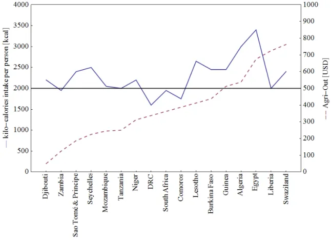
The conclusions that can be drawn from a deep analysis of Fig. 3, even though referring to data of few years ago (2011-2012), are extremely instructive and will be discussed in this and in the forthcoming sections. From a cursory look, a naïve, but worth to be underscored, comment is that there are countries (those lying within the black circle) living at stages of economies of mere survival (the raw numbers support the idea that the survival tax is barely recovered in these countries). This statement is further supported by Fig. 4, where we have reported the kilocalories intake per person per day for the poorest African countries along with the Agri-Out per capita6, which is a measure of GDPC in terms of individual amount of agricultural goods production (note that the survival threshold is about _{2 10}3kcal

⋅ per capita).

Fig. 4: Calories intake per person vs. the agri-out per capita (data from http://www.nda.agric.za/docs/Economic_analysis/africa05.pdf)

According to the previous remarks, the question we should ask ourselves is whether the world can survive continuing to support such an energy demand and these levels of disparity, which are implying and will imply more and more massive migrations from the less developed countries to those living at larger prosperity levels, with the consequent shock in terms of resources, institutions and social conflicts. We

6 _{It is worth stressing that, looking for a correlation between caloric needs (Y) and agri-out (X), it appears that Y is}

independent of X for values from 0 to 300/400 Agri-out where Y remains almost constant, around an average value of 2000 Kcal. Such an empirical observation is a further statement that even for agicultural products, survival needs are

should also ask whether there are technological, social, political and ethical conditions to conceive, on the world-wide scale, an effort, which, without implying any step back in terms of prosperity, welfare and social rights, achieved by the “western” society, allow a wiser control of the planet energy resources and an appropriate redistribution of prosperity [6].

2 THE IPAT EQUATION

In the previous section we have softly suggested that sustainability, at planet scale, requires corrections to the present model of development, by introducing mechanisms capable of reducing the gap between “wealthy” and “poor” countries.

Far from being an ethical statement, such a conclusion is based on a utilitarian determination, based on quite straightforward observations

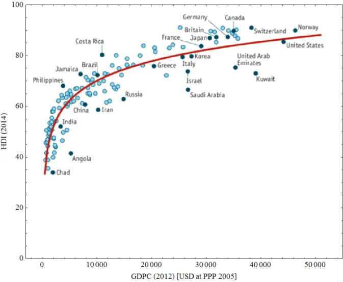
a) the human development index (HDI) improves with GDPC; b) migration fluxes are primarily driven by differences in HDI;

c) the countries with smaller impact on the environment are those who have reached a remarkable level of prosperity.

The statement (a), depicted in Fig. 5, may sound like a tautology, if the concept of HDI is not introduced in quantitative terms, as the geometrical mean of three indicators

3 L S C

HDI = I I I (2)

where

L

I is the life expectancy index,

S

I is the school education index,

C

I is the comfort index.

The statement (b) is also less naïve than it might appear, if properly discussed within the gravitational model of economy [7]; in Sec. 4 we will outline a model concerning the relationship between HDI (which is an alternative measure of the GDPC disparity) and the increase of the pressure by migrant populations, looking for survival perspectives.

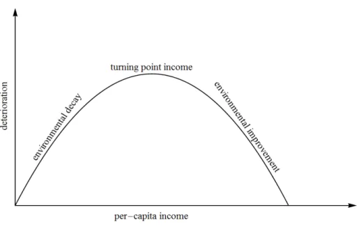
As to point (c), which looks like an oxymoron, it is better understood by referring to the so called Kuznets curve [8], according to which environmental impact vs. per capita income follows the qualitative inverted U shape behavior, reported in Fig. 6.

Fig. 6: Environmental Kuznets curve: the environment deterioration increases with GDPC up to a given threshold and then decreases

The pressure on the ambient due to persisting low GDPC (and thus production processes relying on poor technology) will create unsustainable level of pollution, determining the deterioration of a luxury good of primary importance, represented by the environment quality7.

In this section we will treat this last aspect of the problem and try to quantify the influence of the economic growth on the environment, using the so called IPAT equation [9], which states that the environmental impact (I) depends on population (P), Affluence (A) and technological intensity (T) through the identity

I

=

P A T

⋅

⋅

The affluence is the possibility of a population to have access to goods and the technological intensity is the use of the environment impacting element on the production of goods. The most appropriate way of measuring the affluence is the GDPC. The following example specify how the impact expressed as tons of

2

CO

We evaluate the

CO

(http://data.worldbank.org/indicator/NY.GDP.PCAP.CD) 9 2007 3 2007 2007 6.6 10 , 5.9 10 , 760 / P A USD T g USD = ⋅ = ⋅ = 9 1999 3 1999 1999 5.3 10 , 4.7 10 , 860 / P A USD T g USD = ⋅ = ⋅ =

In these examples the technological intensity is the amount of

CO

of goods [10], we calculate then

9 3 9

2007 6.6 10 5.9 10 760 30 10 ,

I _{= ⋅ × ⋅ × ≅ ⋅} t 9 3 9

1990 5.3 10 4.7 10 860 21.7 10

I _{= ⋅ × ⋅ × ≅ ⋅} t

The technological improvement, which has determined a reduction of the

CO

provided a less significant increase of carbon dioxide emission, in spite of the increase of the population and of the GDPC.

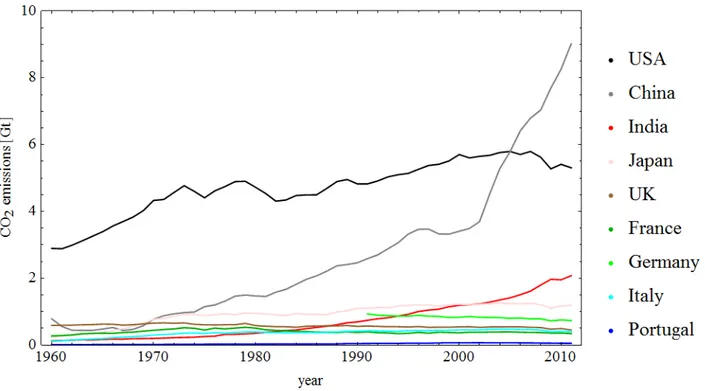
The previous quite naïve derivation has been benchmarked against the data reported in Fig. 7,according to which the amount of carbon dioxide dispersed in the environment has decreased with time in “western” countries, while the “eastern” block (China and India) displays a constant increase.

The IPAT equation may sound like a kind of qualitative statement, however, if properly interpreted, may become a useful tool for decision keepers.

7 _{In our assumptions we have assumed that HDI is a function of GDPC but the dependence might more subtle and}

perhaps further information could be obtained from an analysis in which Kuznets curve depends either on HDI and GDPC as independent variables, as discussed in a forthcoming investigation.

Fig. 7: Gygatons of CO2 equivalent emission per country covering a period of 50 years (data from http://data.worldbank.org/).

The information which can be drawn from Eq. (3) regards the fractional variations of the various quantities entering its definition. The fractional variation of the environmental impact can accordingly be cast in a more convenient form, yielding the IPAT equation in differential terms, namely

I P A T I = P+ A+T ɺ ɺ ɺ ɺ (4) where q q

ɺ _{is the relative variation of the generic quantity in a year,}

which, as we will see, is a fairly useful conceptual tool. It can e.g. be exploited to distinguish between different growth scenarios.

a) Relative Decoupling

This is the context in which the relative variation of the technological intensity is negative but it is not sufficient to determine an analogous trend for the relative variation of the environmental impact, namely

0 , 0 _> < I I T Tɺ ɺ

In this scenario negative values of the relative variation of the technological intensity determine a negative slope of the environmental impact, namely

0 , 0 _< < I I T Tɺ ɺ

Absolute decoupling are therefore the conditions for which the relative impact on the ambient (including population, affluence and technological intensity) decreases.

Relative decoupling, regarding carbon dioxide, seems to have occurred in the last 20 years ( ≈−0.7% T

Tɺ

) [10].

Absolute decoupling is however required in order to limit the increase of the planet temperature, due to global warming. The limit of 4.9% within 2050 is the request to constrain the planet temperature growth within 2% .

According to Eq. (2) we find the full decoupling goal fixed by

4.9% P A T P A T

− = + +

ɺ

ɺ ɺ

we can therefore envisage different strategies to meet the conditions allowing the fulfillment of such a goal. We can, for example, impose a world-wide decrement of the population, a further decrement in the affluence (by imposing a reduction of the global GDP per capita) and finally a wise reduction of the technological intensity.

Unfortunately a strategy of this type is not viable, because

1. the variables of the IPAT equation are not independent each other;

2. the inertia of the demographic or economic systems cannot be straightforwardly counteracted, without creating additional and uncontrolled consequences;

3. the technological intensity is so entangled to economic, social, geographic… factors that it is difficult to establish a long term coordinated action between different nations, including poor, emerging and wealth countries.

In the following we will see how the previous discussion may be translated in more quantitative terms; however, before providing any comment, we fix the methodology we will follow to deal with the problem we are discussing.

We will assume that the population (_P) and GDPC (

G

Regarding e. g. the population dynamics we will select a given period, specified by a number of years

N

[

]

r growth rate year P population at n P final population n N = + − ≡ = = = = > =

(5)

The assumptions underlying a logistic type behavior is that the demographic dynamics is rather naïve, namely an exponential growth followed by a kind of saturation.

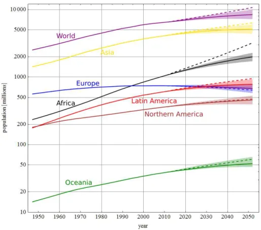
Fig. 8: Population growth from 1950 and projection till 2050 (source https://en.wikipedia.org/wiki/Population_growth).

In Fig. (8) we have reported the world population evolution during the last 60 years, along with three possible scenarios of growth till 2050.

We disregard the high and low cases and consider the “medium” scenario, reproduced by the logistic behavior8

[

]

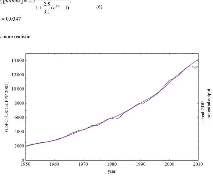
Fig. 9: World real GDP (billions) growth from 1950 to 2015 in Us 2005 dollars adjusted with inflation the interpolating curve represents the potential output. Real GDP fluctuates around the potential output by an average of less 2% (source [2]).

In Fig. 9 we have shown the long term real GDP and potential output9 in PPP (Purchasing Parity Power) 2005 USD, assuming a stationary GDP of 20·1012 USD after 2050, we find the logistic type behavior

[

]

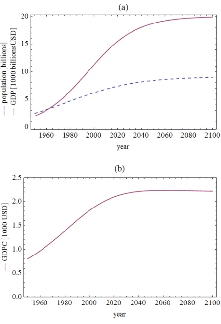
Either GDP and population growth from Eq. (4) and (5) are reported in Fig. 10a while the GDPC (

G /

P

is shown in Fig. 10b.

9 _{Real GDP is the value of final goods and services produced in a given year, when valued at the prices of a reference}

base year. Nominal GDP is the value of goods and services produced during a given year valued at the prices that prevailed in that same year.

Potential output grows at a steady pace because the quantities of the factors of production and their productivity grow at a steady pace. Real GDP fluctuates around potential GDP.

Fig. 10: Population growth and real GDP (a) and GDPC (b).

We have finally provided in Fig. 11 the IPAT incremental component

_∆

4.9% T T P A P A dq q dn − = ∆ + ∆ = + = ɺ ɺ ɺ ɺ (8)

Fig. 11: Sum of population and GDP fractional variations vs years 2000-2050.

According to the results reported in the figure,

_∆

The role played by this variable is extremely complex and we will adopt a very naïve point of view relying on simple considerations based on the Kuznets curve and on the scaling law from Fig. 3.

A further inspection to the data summarized in the figure shows that

1. countries with a middle-high level of GDPC like Bahrain, Kuwait, UAE… (up- right red circle in Fig. 3), have a large amount of resources and employ a significant amount PCC;

2. other countries, with comparable or even larger income (down-right blue circle) employ a smaller PCC.

The difference is presumably due to the fact that the countries of the second block uses more efficient technologies. We can therefore speculate that the exponent factor of the scaling law derived from the data of Fig. 3, can be associated with the technological efficiency.

If we assume 0.76 0.46 , 4000 ( , ) 0.46 b, 4000 GDPC GDPC PCC GDPC b GDPC GDPC  ⋅ ≤ =  ⋅ >  (9)

where the threshold of 4000 USD is read in correspondence of 2000 W in the plot (continuous line) of Fig. 12, where also Eq. (9) is presented (dotted line).

In Eq. (9) the elasticity factor b is different from 0.76 above the GDPC threshold, namely b = 0.6, thus for power consumption above 2000 W. The reasons of this choice is justified by the study of [9], in which the vision for a 2000 W society is promoted. Such a choice (see the concluding section for further comments) could certainly provide a reduction of the power per capita demand.

Fig. 12: PCC vs. GDPC, also with a different elasticity coefficient.

By introducing average value of the power consumption per capita APCC

max max min min 1 ( ) ( , ) GDPC GDPC GDPC GDPC APCC b PCC x b dx − =

∫

and plotting it vs. the technological exponent b in Fig. 13 we can stress that b = 0.6 provides a kind of turning point. Assuming therefore the possibility of keeping the coefficient b between 0.5 and 0.6 for countries with GDPC above 4000 USD, the APCC should slightly overcome 2000 W.

If we use such an indication to evaluate the amount of energy to be used at global level we obtain the forecast shown in Fig. 14 for the years from 2020 to 2120, with an average fractional variation of the technological intensity not exceeding 0.5%.

Fig. 14: alculated energy (a) and its relative variation (b) since 2020.

In conclusion, putting everything together, we end up with a fractional variation of the impact parameter less than 0.1% within 2080 (see Fig. 14). This conclusion is based on a the following assumptions

1. The world population reaches a stationary level in the next years (with reference to Fig. 8)

2. The GDPC income follows an analogous evolution, yielding average values not exceeding 20,000 USD PPP 2006

3. The fractional technological intensity depends on the GDPC income and on the exponent parameter b, as discussed above.

We have, in other words, assumed that the CO₂ equivalent emission does not decrease unless we assume a different dependence of pollutant emission vs. income, as implicitly contained in the paradigm underlying the Kuznets curve.

The limit of ∆ _≅−5% I

I

seems to be rather difficult to be achieved, unless radical changes occur. In the following section we will further comment on these points.

3 THE KUZNETS CURVE: MYTH OR REALITY?

Before entering any discussion regarding the Kuznets Environmental curve (EKC) [8,11], let us try to understand, using a very simple example, what is the amount of

CO

of economy.

In Italy we use 50 l of waters per capita at the temperature of 45 degrees centigrade for cooking and hygienic purposes10. Assuming that water is distributed at 15 degrees, the amount of energy employed for the relevant heating is therefore 1.744 KWh. The amount of

CO

process spans from 0.96 kg/day to 0.36 kg/day, according to the type of technology employed. In conclusion, for food and personal hygiene we disperse in the environment an average of 3 10_⋅ 8 _{kg/day of}

2

CO

Just to fix a reference value, we can quote about

700

Kg

CO

/

MWh

2

electric; if we trust the

allometric law from Fig. 3 we can conclude that the

GDPC

3 0.76

2

10.44 10

CO

GDPC

t

≅

⋅

⋅

We find therefore that China with a GDPC of 5.69 10 USD3

⋅ in 2011should be responsible for the emission

of about 7 tons of CO_{2, repeating the same exercise for India we find 2.5 tons per capita which is a}

somehow an overestimated value with respect to the data reported by World Bank Org.

In these countries the carbon di-oxide emission has been characterized by a large increasing rate over the years following the growth of GDPC (Fig. 6). In other countries the trend seems to follow a different pattern, after a certain threshold the emission (per capita) decreases with increasing GDPC.

On purely qualitative grounds economists have provided empirical evidence of “a systematic relationship between income changes and environmental quality” [11].

What has emerged is a trend according to which both environmental quality and incomes, after an unspecified threshold, improves. In other words “the wealthier we get, the more environmental quality we demand” [11].

Since the original proposal there has been a significant amount of studies trying to provide a more sound and quantitative base to such a point of view.

The most significant output of these researches is that various forms of curves emerge, depending on the type of pollutant, geographical and political conditions.

Leaving for the moment the criticisms apart, we consider an example of how EKC can be exploited within the framework of the speculations developed in the previous section, to this aim we consider a specific curve shape obtained in the past and regarding the Sulphure dioxide emission vs. the GDPC (Fig. 15) [12]. From the analytical point of view [13] such a curve can be reproduced by

(

)

being α and τ two fitting parameters.

The use of the above analytical form and the trend evaluated in the previous section for the development of GDPC vs. years, we obtain the result summarized in Fig. 16, which foresees a drop in the next decades. The example we have reported is only an indication of how data and fitting formula can be “patched” together to get a predictive model, whose reliability should however be taken “cum grano salis”. For a more complete analysis including the effect on climate changes and the interplay with economy see [14].

Fig. 15: Real SO₂ emission (source [12]) compared to the plot from Eq. (11) with τ=300, α=50.

We like to conclude this section with a few elements of caution regarding the methodology which has been followed in this article and in most of the quoted literature. We have to stress that the temptation of simplifying the model in absence of a sound theoretical basis is strong. The EKC has no theoretical

foundation but wise empirical observations, in addition the data supporting its evidence, are confusing if analyzed in depth. The best we can say that a trend perhaps exists.

Fig. 16: Kuznetz curve of SO₂ emission. vs. years assuming the GDPC growth of Fig. 9 (the shape is extremely sensitive to the model parameters, therefore any prediction is merely indicative).

To make stronger such a statement, we have collected in Fig. 17the emitted CO_{2per capita vs. the GDPC}

for European countries; it seems evident that after a rise up a kind of stationary condition is reached, but nothing more can be concluded. The volatility of the political and economic choices, of the associated scenarios prevents any serious forecast and perhaps the GDPC is not a good indicator.

Fig. 17: Linear-linear plot of CO₂ emission per capita vs. GDPC for some European countries (data from http://data.worldbank.org/).

The further point we would like to comment is the use of “scaling laws” like the one derived from the plot in Fig. (3). There is no doubt that beyond these type of analysis there is some fashion. They allow indeed the possibility of connecting different variables and of speculating about the possible correlations [15,16]. Most of the interpretation is associated with the values of the fitting coefficients (the celebrated factor ¾=0.75 is one of the most quoted recurrent value in the associated speculations, see [15] and references therein). We have therefore tried an independent check with European countries (see Fig. 18) and the regression curve we have obtained exhibit a better R factor but with different fit parameters, which seems to be time dependent. A factor around ¾ is obtained for more recent years when a strong homogeneity has occurred.

Fig. 18: CO2 emission per capita vs. GDPC for different European countries in 1991 and 2009 (data from http://data.worldbank.org/).

The data of the years after the economic recession (2011, along with the 2009, for a better comparison) are reported in Fig. 19 and the associated consequences are evident: the points are more scattered and the slope is lower.

We have added this caveat not to deny the use of scaling or regression formulae, but to stress that they are a useful, but potentially misleading tool, if used with an “ideological” byes, we believe however that the time dependence of the fitting coefficients is a poorly understood subject, which should be appropriately investigated.

Fig. 19: CO2 emission per capita vs. GDPC for different European countries in 2009 and 2011 (data from http://data.worldbank.org/).

4 FINAL COMMENTS

The discussion of the previous section suggests that ECK may be viewed as a kind of paradigm of how things should go if, after an intense grow up of the economy in a certain country, the policy of that country is that of looking for new solutions to counteract the environment degradation. Even if such a paradigm applies, the problems of environmental degradation, at global scale, remain the same. Because the pollution is not local and in emerging countries, with large populations, it is not clear how aggressive may be the environment pressure.

A more correct framing of the ECK should be what economists define “Stylized Facts” [17], namely empirical regularities that can be inferred without employing educated econometric techniques. Econometrics can, successively, help to validate (deny) them. These occurrences cannot be considered to be valid for all countries and at any time, but suggest statistical tendencies and do not necessarily underlie “structural relationships”. In conclusion they may be viewed as “experimental evidences” which may hide complex dynamics, eventually leading to functional relationships between the variables under study. In alternative, they may be considered historical characteristics of the data that any model of energy and economic growth must be able to reproduce.

Most of our considerations have been developed for countries with too different backgrounds and the search for structural relationships demands for a “clusterized” studies in which the countries are sampled on the basis of their homogeneity, which is also a rather qualitative variable hard to be defined in quantitative terms. In this paper we have relied upon the use of scaling relations, in particular that represented by the power vs. GDPC reported in Eq. (1) and by the relevant regression fit in Fig. 3. It is evident that when so large and inhomogeneous data are treated problems arise for the proper understanding of the meaning of the fit itself. Grouping countries with similar political and economic status the fit is characterized by a larger R-factor with almost similar b coefficient but a different a value. The result is that reported in Fig. 20 in which we have superimposed to the plot of Fig. 3, the up (inefficient technology countries) and down (efficient technology countries) curves with the fit of [4] interpolating in between.

We have loosely defined inefficient and efficient technological countries, those lying above or below the central regression curve but this should not be taken literally. The countries like UAE do not care too much about the consumption because they have a significant amount of natural resources, moreover Russia employs larger power per capita for heating problems. The exact contrary occurs in Polynesia.

We have stressed the meaning of the b factor as a kind of elasticity coefficient, but we did not dwell on that associated with a, which should be interpreted. It is a parameter of central importance too and, as reported in Figs. 18, can be brought around unity, if the fit is done within the group of developed countries only. On the other side if below a certain income threshold the power per capita is independent and above a certain threshold efficient technologies are used a kind of decoupling has been obtained and the power-GDPC log-log plot is quasi linear with a convexity down.

Fig. 20: Efficient and inefficient technologies and decoupling (source [4]).

It is evident that the fit coefficients of the regression formulae are a very delicate elements of the discussion and should be handled with extreme care. We have put much emphasis on the values characterizing the fit reported in Fig. 3, the agreement on these results is however not unanimous. The speculations regarding the supposed ubiquity of the scaling factor, albeit interesting and sometime well documented, may be a kind of byes for the analysis of the data itself. Our caveat is supported by other researches [19] and in Fig. 21 we have reported the nutritional energy supply per capita and per day vs. the GDPC reported in [18].

The regression fit of the data for_{Y a X}d

= ⋅ is with a = 850 and d = 0.14.

It should also be remarked that caloric intake that above a certain GDPC threshold the data are not too much significant and the curve exhibits a low elasticity. The slope cannot be the same including survival and well developed economies

A more accurate fit in the region of low income (less than 5000 USD) could therefore reveal further interesting elements of speculation, which are however out of the present analysis. For further comments the reader is addressed to [18] where the statistical significance and reliability of the analysis of the data is discussed in depth in terms of elasticity of the nutritional energy vs. the GDPC, which is evidently large around the lower values of the curve.

It is certainly true that the analysis of calories intake vs. income is flawed by physiological limits and that this is not true for the power demand.

A better figure of merit is the energy per capita per year vs GDPC, the relevant plot is given below and does not require any further comment except that it is “almost linear or convex down” [18]. The convexity may be an indication that the effect of “decoupling” policies of some advanced country may become apparent. However, as also stressed in [19] the effectiveness of the decoupling requires a major effort involving further countries.

Fig. 21: Nutritional energy per day supply per person vs. GDPC (source [18]).

The consistency of the plot in Fig. 22 with the previous results can be considered satisfactory and a regression fit of the region above 1000 USD yields fit parameters analogous to those quoted in the previous sections.

Fig. 22: Energy use per capita in one year vs. GDPC (source [18]).

As a further comment regarding the analysis of the macroeconomic data we can conclude that a reasonable reference value for the world-wide energy requirement per capita is no more than 2000 watts. In western countries the actual demand is for more than twice. An energy reduction allowing towards such a target is possible without any prejudice for the present day standard of life. For this reason a strong commitment involving solutions from different areas (science, economy, politics…) is required [6].

Before concluding the paper let us remind a problem in which significant effort should be invested and regarding migration. As already remarked if the economic disparity between “rich” and “poor” countries will continue migratory fluxes are expected to produce to be such devastating consequences in terms of life sustainability for the hosting countries.

If we are interested in framing the problem into quantitative terms, we should refer to model like those employing analogies with physical systems.

At the beginning of forties of last century it was noted by an astronomer of Princeton that the distance of his students’ home town from Princeton University mightbe derived from a “law” analogous to that of Newton gravity [20]. The observation was essentially that the interaction among from demographic agglomerates was ruled by an equation of the type

2 , , j i j i j i D P P F ∝

Where

_P

,

is the distance between the i, j locations. The above identity states that the demographic force is proportional to the product of the populations of provenience and destination and inversely proportional to the square of their distances.

There are some misconceptions about the correct understanding of this type of relationships, which can be better understood if framed within the context of the Gauss law. If we look at the migrants as to a demographic flux from a given surface we can obtain a less abstract correspondence.

There is no doubt that migration is the result of complex problems and models are just a way to settle out pivotal parameters. We propose therefore a different model analogy based on a kind of Ohm law, in which the current corresponds to the number of migrants per unit of time, the voltage difference corresponds to the difference in GDPC (or the HDI as well), the resistance is “measured” in terms of GDPC/(migrants/time). It is evident that the most naïve circuit realizing such an analogy is an R-C with a potential V. In the case of north Africa-Italy migration the role of the capacitor is played by Italy and it is represented by the carrying capacity of the Italian structures themselves. Regarding the analogous of the power lost in the circuit we note e. g. that the product current per potential difference is replaced by the GDPC*(number of migrants/time), which yields the amount of investment (by the hosting country) necessary to support the migration.

The model employs few parameters and can be elaborated as a predictive tool, as it will be shown elsewhere.

ACKNOWLEDGMENTS

The Authors express their sincere appreciation to Dr. D. Giacomantonio for a careful reading of the manuscript, useful remarks and enlightening comments.

5 REFERENCES

[1] P. Malanima (2009), "Energy and Population in Europe. The Medieval Growth (10th-14th Centuries)", L’Europa come problema, Villa Vigoni, Menaggio.

[2] R. E. Hall, M. Liberman (2013), "Economics Principles Applications", South-Western Cengage Learning.

[3] G. Dattoli, M. Del Franco, J. V. Rau (2012), “Elementi di Fisica Tecnica mbientale”, RT/2012/14/ENEA, Enea, Roma.

[4] J. H. Brown et al. (2011), "Energetic Limits to Economic Growth", Bioscience 61, 19-26.

[5] G. B. West GB, J. H. Brown, B. J. Enquist (1997), "A general model for the origin of allometric scaling laws in biology", Science 276, 122–126.

[6] P. C. Beyeler, H.-P. Fricker (2007), "The 2000 Watt Society – Standard or Guidepost?", Energie-Spiegel 18, 1-4, Paul Scherrer Institute, Swiss.

[7] J. E. Anderson (1979), “A Theoretical Foundation for the Gravity Equation,” American Economic Review, 69(1), 106-16.

[8] B. Yandle, M. Vijayaraghavan, M. Bhattarai (2002), "The Environmental Kuznets Curve - A primer", PERC Research Study 02-1.

[9] M. R. Chertow (2001), “The IPAT equation and its variants”, Journal of Industrial Ecology 4, 13-29. [10] T. Jackson (2009), "Prosperity without growth: economics for a finite planet", Earthscan, London. [11] C. Hepburn and A. Bowen (2012), “Prosperity with growth: Economic growth, climate change and environmental limits”, GRI Working Papers 93, Grantham Research Institute on Climate Change and the Environment.

[12] J. Begun (2007), "In Search of a Sulphur Dioxide Environmental Kuznets Curve:

A Bayesian Model Averaging Approach", Working Paper no. 79 , Center for Statistics and the Social Sciences , University of Washington.

[13] K. Gorska, H. Horzela, K. Penson, G. Dattoli, G. H. Duchamp (2016), "The stretched exponential behavior and its underlying dynamics. The phenomenological approach", ArXive: 1603.06066v4 [cond-mat.stat-mech].

[14] Committee on Stabilization Targets for Atmospheric Greenhouse Gas Concentrations (2011), "Climate Stabilization Targets: Emissions, Concentrations, and Impacts over Decades to Millennia", National Academy Press, Washington DC.

[15] G. I. Barenblatt (2013), "Scaling", Cambridge University Press.

[16] Dattoli, P. L. Ottaviani, S. Pagnutti (2009), “Leggi di scala in Biologia e sviluppo delle masse tumorali” Il Nuovo Saggiatore 25, 24-35.

[17] Z. Csereklyei, M. d. Mar Rubio Varas, D. I. Stern, "Energy and Economic growth: Stylized facts", CCEP Working Papers 1417, Crawford School of Public Policy, The Australian National University.

[18] P.W Grbens-Leenes, S. Nonhebel, M. S. Krol (2010), "Food consumption patterns and economic growth. Increasing affluence and the use of natural resources", Appetite 55, 597-608.

[19] United Nations Environment Programme (2011 ), “Decoupling Natural Resource Use and Environmental Impacts from Economic Growth”, Earthprint.

[20] J. E. Anderson (1979), ‘‘A Theoretical Foundation for the Gravity Equation’’, American Economic Review 69(1), 106–16.

ENEA

Servizio Promozione e Comunicazione

www.enea.it

Stampa: Laboratorio Tecnografico ENEA - C.R. Frascati giugno 2017