An Integer Linear Programming Model for View Selection on Overlapping Camera Clusters

An Integer Linear Programming model for View Selection

on Overlapping Camera Clusters

Massimo Mauro

_{, Hayko Riemenschneider}

_{, Alberto Signoroni}

_{, Riccardo Leonardi}

_{, Luc Van Gool}

_{Department of Information Engineering, University of Brescia, Italia}

2

_{Computer Vision Laboratory, ETH Zurich, Switzerland}

_{K.U. Leuven, Belgium}

Abstract

Multi-View Stereo (MVS) algorithms scale poorly on large image sets, and quickly become unfeasible to run on a single machine with limited memory. Typical solutions to lower the complexity include reducing the redundancy of the image set (view selection), and dividing the image set in groups to be processed independently (view clustering). A novel formulation for view selection is proposed here. We express the problem with an Integer Linear Programming (ILP) model, where cameras are modeled with binary vari-ables, while the linear constraints enforce the completeness of the 3D reconstruction. The solution of the ILP leads to an optimal subset of selected cameras. As a second contribu-tion, we integrate ILP camera selection with a view cluster-ing approach which exploits Leveraged Affinity Propagation (LAP). LAP clustering can efficiently deal with large cam-era sets. We adapt the original algorithm so that it provides a set of overlapping clusters where the minimum and max-imum sizes and the number of overlapping cameras can be specified. Evaluations on four different dataset show our so-lution provides significant complexity reductions and guar-antees near-perfect coverage, making large reconstructions feasible even on a single machine.

1. Introduction

Scalability is an issue for Multi-View-Stereo (MVS) al-gorithms [20,25,7] and a limitation for large image-based 3D reconstructions [1,4]. A first way to address the prob-lem is to reduce redundancy in the input data. View selec-tion algorithms have the goal of removing repetitive images. However, view selection is not enough when the image set is very large. Since MVS algorithms work by using the whole set of images at once, a further help can come from parti-tioning the views in clusters to be processed independently and eventually in parallel.

The combination of clustering and selection can lead to three main benefits: 1) reconstruction time on a single

ma-chine is reduced due to the smaller dimensions of the clus-ters; 2) large reconstructions are made possible on single machines with limited memory; 3) the processing may be split across multiple machines for further speedups.

In this work1_{, we propose a novel approach for view} se-lection, formulating the problem with an Integer Linear Pro-gramming (ILP) model. According to ILP, each camera is represented by a binary variable, which could be selected or not. The linear constraints enforce the shared visibility of points between cameras to guarantee the coverage of the final 3D reconstructions. Solving the ILP model we find a globally optimal set of cameras, avoiding any heuristics or greedy iterative procedures used in other works [26,9,8,6]. As a second contribution, we integrate the ILP selec-tion model with a view clustering soluselec-tion based on Lever-aged Affinity Propagation (LAP). LAP is an extension of Affinity Propagation clustering [5] able to deal with large-scale data. We increase the flexibility of the LAP algorithm by handling additional constraints on minimum and max-imum cluster size and by admitting overlapping clusters. Cluster overlaps are important for reaching a well-covered reconstruction near cluster boundaries, especially in semi-structured camera scenarios [15].

We test our algorithm on different types of image sets: structured, unstructured, streetside and aerial. Experiments show that our method leads to a reduced and well-grouped cameras sets, while guarantees the overall coverage, scala-bility, and high quality of the 3D reconstructions.

1.1. Related Work

The problem of scalability for large-scale 3D re-construction has been addressed in a few other works. We briefly discuss the most relevant methods for scal-ing both Structure-from-Motion (SFM) and Multi-View Stereo (MVS) algorithms.

1_{This work was supported by the European Research Council (ERC)}

under the project VarCity (#273940) at www.varcity.eu and by the Italian Ministry of Education, University and Research under the PRIN project BHIMM (Built Heritage Information Modeling and Management.)

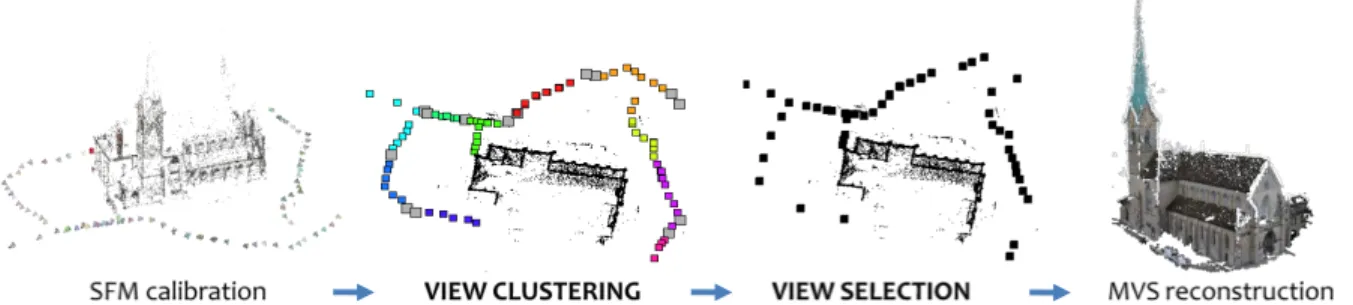
Figure 1. Outline of the view clustering and selection for scalable MVS reconstruction. Different colors indicate different clusters while gray squares are the overlaps. For view selection, black squares show removed cameras.

SFM scalability. Snavely et al. [24] find skeletal sets of images from a given unordered collection which pro-vide a good approximation of the SFM reconstruction us-ing the whole image set. They first estimate reconstruc-tion accuracy between pairs of overlapping images, from which they form a graph and find the skeletal by means of a maximum-leaf t-spanner algorithm. Li et al. [14] find a small subset of iconic images comprising all the impor-tant part of the scene. They initially proceed by applying 2D appearance-based constraints to loosely group images, and progressively refining these groups with geometric con-straints to select iconic images giving a sparse visual sum-mary of the scene. Crandall et al. [3] introduce a Markov Random Field (MRF) formulation for SFM which finds a coarse initial solution and then improve that solution us-ing bundle adjustment. Their formulation incorporates vari-ous sources of information such as noisy geotags or vanish-ing point estimates. Contrary to these, our work deals with the scalability for MVS and exploits the information about 3D points and cameras derived from SFM. Hence, the pre-sented approach could be potentially combined with any of the above methods.

MVS scalability. Clustering and selection techniques have been proposed for addressing MVS scalability. In their selection method, Hornung et al. [11] rely on coverage and visibility cues to guarantee a minimum reconstruction qual-ity and then refine the most difficult regions using photo-consistency. Tingdahl et al. [26] reduce the set of initial views relying on depth maps data. Goesele et al. [9] and Gallup et al. [8] select viewpoints relying on simple prop-erties of the input images such as resolution or baseline. Ladikos et al. [13] propose a spectral clustering approach which incorporates scene and camera geometry to build a similarity matrix and then use mean shift to automatically select the number of clusters. Recently, Riemenschneider et al. [19] provide a partial view selection method which se-lects parts of an image for the goal of optimizing scene un-derstanding.

Most closely related to our work of view clustering and selection method are the works of Furukawa et al. [6] and Mauro et al. [15]. Furukawa et al. [6] model the problem

as an iterative optimization. At first they remove redundant images, then they build a graph representation of remaining cameras and divide them into clusters through normalized-cuts while respecting a constraint on the maximum size of clusters. As a final step, an image addition process creates overlaps between clusters to respect a coverage constraint.

In contrast to them, we place clustering before selection. In this way selection is run on a smaller camera set, and both selection and reconstruction can be parallelized. Since our clustering finds very precise overlaps on cluster borders, selection can be safely parallelized: being careful not to re-move overlapping cameras, the creation of holes between clusters can be reliably avoided. As a second difference from Furukawa et al. [6], our ILP selection model is not it-erative: it jointly evaluates all cameras and constraints find-ing an optimal global solution.

Mauro et al. [15] also build a graph based on camera angle similarity and find regular overlapping clusters using dominant sets [18] (DS). View selection is not included in their work. The DS approach requires an iterative proce-dure: a single run of DS divides the graph in two, a dom-inant set and a ”remaining set”. Multi-cluster subdivision is then obtained by iterating on the remaining set. In some cases, this process may isolate some cameras leading to a wrong assignment of cameras to clusters (Figure2).

Conversely, we adopt Affinity Propagation clustering [5] which considers all data points at once and avoids the above problem. For large image sets, we use Leveraged AP, a ver-sion of AP which finds a solution on sampled subset of data and then infers cluster assignment for the whole set.

Hence, the contributions of our paper are the following: 1. a novel optimal formulation of selection with Integer

Linear Programming,

2. a novel overlapping cluster assignment exploiting Leveraged Affinity Propagation,

3. the integration of our ILP selection and clustering in a joint system of which we release the code.

2. Overlapping view clustering with AP

The goal of camera clustering is to produce an appro-priate number of groups to be processed independently and in parallel. Additionally to the inherent intra-similarity re-quirements, we want to satisfy the following constraints:

• minimum size constraint: every cluster must be greater than Nmin cameras (with Nmin 2 for making

matching possible).

• maximum size constraint: every cluster must be smaller than Nmax. This constraints allows to run

memory expensive dense reconstructions on machines with limited memory capabilities.

• overlap constraint: every cluster must indicate a num-ber Noverlap of overlapping cameras with other

clus-ters. This procedure improves the density of the recon-struction at the ”borders” of a cluster.

We divide the presentation of the clustering algorithm in three sub-parts: the point cloud pre-processing, the defini-tion of the camera similarity matrix, our novel multi-cluster solution with constraints.

2.1. Pre-processing of the SFM point cloud

We are given a set C of NC cameras and a 3D sparse

point cloud P of size NP resulting from

Structure-from-Motion (SFM). Considering a camera Ci, we note as VCi

the set of points which are visible from the camera (camera visibility). Dually, considering a point Pi, we note as VPi

the set of cameras looking at the point (point visibility). Cloud scaling. As a first step, the input point cloud is normalized. The normalization scales the point cloud to have a unit distance ( ¯R = 1) as average distance between its points and their nearest neighbor. This allows the conse-quent methods to use distances regardless of scale. Also the camera positions are scaled accordingly.

Merging visibility information. As also noted by [6], undetected or unmatched image features may lead to errors in the visibility estimates: adjacent points may have dif-ferent point visibility sets, leading to imperfect similarity estimates. We thus simplify the structure with a 3D grid voxelization: the new merged points are positioned at the centroids of voxel cells with side dimension L, while the point visibilities becomes the union of the point visibilities inside each voxel. Reducing the size of the PSF M cloud

lowers the computational effort of the subsequent steps.

2.2. Similarity matrix

The N ⇥ N symmetric matrix S of pairwise similarities between cameras takes into account both angle and distance information and is defined as S = S↵· Sd, where S↵is the

angle matrix and Sdis the distance matrix.

(a) Dominant Sets

(b) Affinity Propagation

Figure 2. Clustering results with line connections on Fraumunster dataset [15]. Wrong cluster assignments due to the iterative DS clustering are solved with AP.

Angle matrix. Given a pair of cameras (Ci, Cj), the

angle similarity s↵i,j is defined as:

s↵i,j =

P

p2(VCi\VCj)s↵ijp

| VCi\ VCj |

(1) where p 2 P and s↵ijp is dependent on the angle ↵ijp

be-tween the viewing directionsCi !pandCj !pdefined as

s↵ijp = exp( ↵2 ijp 2 ) (2) ↵ijp= arccos (Ci p) T_(C j p) k Ci pkk Cj pk (3)

There is an angle limit between 30 and 40 beyond which the same point is difficult to match among different images [17]. We thus set = 30 in our experiments.

Distance matrix. All the values in S↵are in the range

[0, 1]. To have the same range in Sd we first evaluate the

median distance ¯d, i.e. the median value of the distances between every camera and all the other cameras. Then we define the distance similarity sdi,j as:

sdi,j = 8 < : 1 if i = j 1 1+exp ✓ (D(Ci,Cj ) ¯d) ¯ d ◆ otherwise (4)

where D is the L2norm between the camera centers.

2.3. Affinity Propagation for overlapping clusters

Affinity Propagation (AP) considers all given data points at once. As already said, this solves a potential issue of the DS approach [15]. In some situations, such as ordered or semi-ordered camera sets, the iterative process involved by DS may isolate some cameras leading to a wrong assign-ment of cameras to clusters. An example is in Figure2.

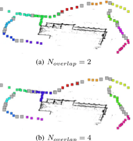
(a) Noverlap= 2

(b) Noverlap= 4

Figure 3. Affinity propagation clustering with increasing overlap constraints on Fraumunster dataset. Note the presence of overlaps on both borders of all clusters.

AP takes as input the similarities between data points and simultaneously considers all data as potential exem-plars (i.e. cluster centers). Real-valued messages are ex-changed between data points until a high-quality set of exemplars and corresponding clusters gradually emerges. Affinity propagation also considers a real p(k) for each data point k so that data points with larger values of p(k) are more likely to be chosen as exemplars. These values are referred to as preferences. The number of identified exem-plars (i.e. the number of clusters) is influenced by the values of the input preferences (usually taken as the median of the affinities), but more importantly it also emerges from the message-passing procedure.

Two kinds of message are exchanged between data points, called responsibility and availability. When the al-gorithm terminates, the responsibility r(i, k), between data point i and exemplar point k, reflects how well-suited the data point is as a member of its cluster (how much the point ”likes” its exemplar). The availability a(i, k) between ex-emplar point k and point i, reflects how good the candidate exemplar is for the point. We refer to [5] for more details.

Cluster constraints. The original AP algorithm auto-matically finds the appropriate number of exemplars, and all the cluster form disjoint groups. Instead we need over-lapping clusters with pre-determined sizes.

Size constraint. First, too small cluster are merged to nearest clusters i.e. clusters with the nearest exemplar -until the minimum size constraint is satisfied. Second, for too large clusters, we increase preference values by forcing large clusters to be split into two.

Overlap constraint. In the similar vein as [15], we im-plement a diverse overlapping approach and find a specified number of cluster borders. The first cluster border is se-lected as the most dissimilar camera to the cluster exemplar, according to S. The next borders are iteratively chosen as the least similar cameras to the previous selected ones. A

0 1000 2000 3000 4000 5000 6000 7000 8000 9000 0 100 200 300 400 500 600 700 800 Number of samples Seconds AP LAP (a) Speed 0 20 40 60 80 100 1.8 1.9 2 2.1 2.2 2.3 (b) AP Clusters (1000 points) 0 20 40 60 80 100 1.8 1.9 2 2.1 2.2 2.3

(c) LAP Clusters (1000 points)

Figure 4. Speed and cluster comparison between Average Propa-gation and Leveraged AP.

diverse selection ensures that in semi-structured scenarios both cluster borders are covered by overlaps, see Figure3.

Leveraged Affinity Propagation. For a large number of cameras, we adopt the so-called Leveraged Affinity Propa-gation. This is a better option w.r.t. sparse AP, since it is not known a priori if the similarity matrix S is sparse. Lever-aged Affinity Propagation samples from the full set of po-tential similarities and performs several rounds of affinity propagation, iteratively refining the samples. A compari-son of AP and LAP methods is done in Figure4: the speed is compared for randomly generated data of different sizes, while the clustering results are shown for a set of 1000 ran-dom points. LAP delivers the same clustering results yet provide a speedup for large datasets.

3. The ILP model for View Selection

Integer Linear Programming (ILP) is an optimization model where both the objective function and the constraints are linear, and the variables are integer numbers. The prob-lem of view selection fits perfectly into an ILP model: our variables are the cameras which could be selected or not, reducing ILP to a binary combinatorial problem.

The previous clustering step with precise overlaps allows to run the selection independently on every cluster. As a re-sult the complexity of the ILP optimization problem, which depends on the number of variables, is reduced. We note as {Cn} the set of cameras associated with cluster n, and

{Pn} the set of seen points (the union of camera

visibili-ties). Three constraints are specified for view selection: • coverage constraint: image selection must not create

holes or missing parts in the structure;

• size constraint: the resulting number of images in a cluster must satisfy the minimum size constraint Nmin

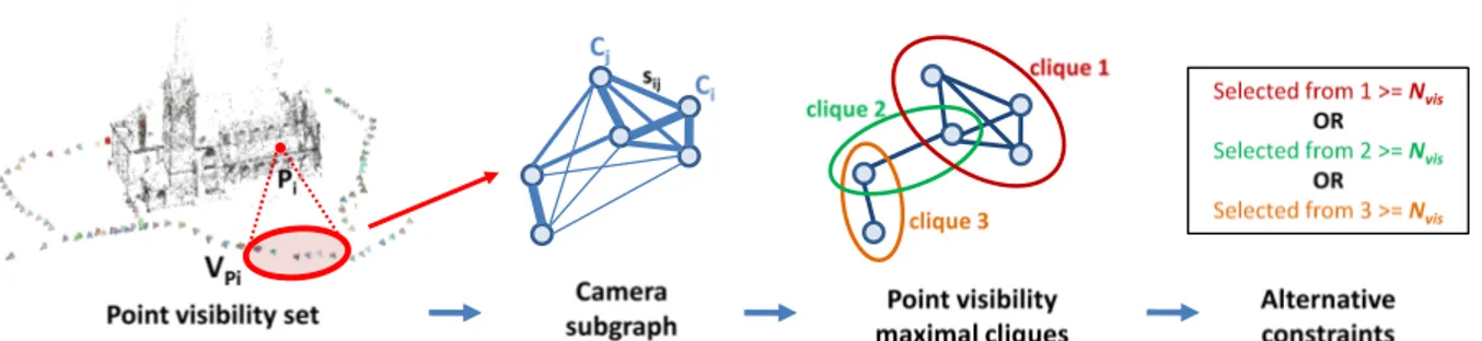
Figure 5. Scheme of the needed process for the formulation of the coverage constraint. Different edge widths in the camera subgraph represent the associated similarities. See text for explanation.

• overlap constraint: overlapping cameras in a cluster must be selected, to maintain the reconstruction quality at cluster borders.

All the constraints are explained as linear inequalities in the ILP model. The resulting ILP problem is formalized as:

minimize cTx (objective function) subject to Ax b (coverage constraint)

Cx d (size constraint) Ex = f (overlap constraint) and x_{2 0, 1}

Vectors x and c are the camera vector and the cost vector respectively, both of length NCn=|{Cn}|. The cost vector

cis filled with 1s, so that the total cost is simply the number of selected cameras. However, any other cost attribution can be used, e.g. by attributing different importance according to the estimated saliency [16,22].

Coverage constraint. Coverage is the most critical among the three constraints. Given the set of cameras in a cluster, one could express the coverage constraint by en-suring that all the NPnpoints of cluster n are seen by at least

Nviscameras in their point visibility sets (with Nvis 2).

Such a constraint is potentially dangerous, because it im-plicitly assumes that all cameras in the point visibility set can be matched to each other. This may not be true: es-pecially in semi-structured scenarios where cameras are al-most along a line, the angle between cameras at different borders of the same cluster may be too wide for a success-ful matching. What the coverage constraint then needs to ensure is that all the NPnpoints of cluster n are seen by at

least Nvismatchable cameras in their point visibility sets.

For a linear formulation, we extract for each point Pi

the subgraph Gi of cameras in point visibility set {VPi}.

Graph Gi is edge-weighted, with weights assigned

accord-ing to values in S. From Giwe derive an unweighted graph

˜

Giby placing a threshold Tmatchon edge values, such that

cameras which are connected in ˜Gi can be assumed to be

matchable. We then extract all maximal cliques from ˜Gi

with the Bron-Kerbosch algorithm [2].

The coverage constraint is defined by ensuring that every point in Pn is seen by (at least) Nviscameras in one of its

point visibility maximal cliques. Since in a maximal clique every node is connected to all other nodes by definition, re-taining Nvis cameras from one of the cliques is the

mini-mum condition to guarantee the coverage. The condition for coverage requires the use of alternative constraints: for ev-ery point Pithere will be a number of alternative constraints

equal to the number of maximal cliques Ncl in its camera

subgraph Gi, reflecting the fact that the condition needs to

be respected indifferently for only one of the cliques. The definition of either - or conditions in an ILP model is made possible with the introduction of auxiliary binary variables y1, ..., yNcl into the constraint equations.

X j2NCn a1jxj b1+ M1(1 y1) . . . X j2NCn aNcljxj bNcl+ MNcl(1 yNcl) X k2[1...Ncl] yk 1 yk2 0, 1

where ak,j = 1only when camera Cjbelongs to the point

visibility maximal clique of the considered point (otherwise ak,j = 0), and bk= Nvis. By specifying Mk= Nvisand

with yk = 0, the constraint on clique k is weakened as the

right-hand side of the inequality renders the condition al-ways true. Conversely, an yk = 1”activates” the constraint.

We then impose that at least one of alternative constraints is ”active” to guarantee the coverage for the point. A graphi-cal representation of the needed steps for the coverage con-straint is in Figure5.

Size constraint. Size constraint is set such that the sum of xi 2 x is greater then the minimum cluster size. Hence,

Cis filled with 1s and d = Nmin.

Overlap constraint. This condition forces the overlap-ping cameras to be selected. Matrix E reduces to a vec-tor where ei,j = 1 for overlapping cameras (otherwise

(a) CMVS (b) DS (c) AP

Figure 6. Affinity propagation clustering compared to CMVS [6] and DS [15] on Fraumunster dataset.

(a) CMVS (b) DS (c) AP

Figure 7. Affinity propagation clustering compared to CMVS [6] and DS [15] on Notredame dataset.

4. Experimental Evaluation

In this section, we experimentally validate the cluster-ing and selection methods. For clustercluster-ing, we highlight the regularity of clusters and overlaps compared to other two recent methods: CMVS [6] and DS [15]. As to selec-tion we compare the full CMVS tool based on heuristics for selection and evaluate the coverage of the obtained 3D models and the runtime gains to a reconstruction run on the full set. We test on four different datasets corresponding to four different scenarios: Fraumunster [15] (structured land-mark), Yotta [21] (streetside), Notre Dame (unstructured landmark) [23], and Wundschuh [10] (aerial).

Parameters Settings. There a few parameters to define in our method. The parameter that most affect the the final results is the voxel dimension L (Section2.1): increasing this value, the selection algorithm has more room for re-moval since the camera subgraph associated to every point is bigger. After some preliminary experiments, we set a L = 15 ¯Ras we found to guarantee good coverage perfor-mances for all datasets. We set Nmax= 40, Nmin= 3and

Noverlaps = 2as clustering parameters. As regards

selec-tion, we use Tmatch= 0.7as threshold for the derivation of

the edge-unweighted graph in Section3, and Nvis = 2as

the minimum number of cameras seeing every point.

4.1. Clustering

Clustering results are shown for Fraumunster and NotreDame in Figures3,6,7. In Figure3clustering results are shown using two different Noverlapsvalues,

highlight-ing the precise positions of cluster overlaps on borders. In Figure6and7cameras in each cluster are connected with a line to better compare the regularity of the clusters in the three different methods. In general, our clusters and over-laps always show a better cluster configuration w.r.t. CMVS

as we model angle and distance and not just pure shared visibility. DS improves upon CMVS, but still some wrong assignments remain due to the iterative problem. Cluster compactness is beneficial during selection, since every clus-ter has little influence on the others and thus selection can be run independently on each of them. Moreover, the pre-cision of overlaps avoids any problem of incomplete recon-structions between clusters.

4.2. Selection

To quantitatively evaluate image selection, we would re-quire a ground truth, which is not readily available for these experiments as there is no best minimal set of images with an optimal point cloud. In this work, for every dataset we reconstruct a 3D point model with the Patch-based Multi-View Stereo (PMVS) method [7] using the complete set of images. This most complete point cloud reconstruction serves as reference.

We define coverage as a metric for evaluation. Given a ground truth point cloud G, and a point cloud P, coverage is computed as follows: for every point giin G, we evaluate

the distance dGP to the nearest point in P. The point gi is

”covered” if such distance is below a given threshold dGP.

The coverage metric is given by the percentage of covered points in G. We set dGP = 4 ¯R.

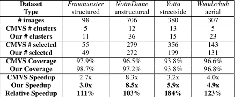
Quantitative results are shown in Table1. We obtain al-most complete coverage with respect to the PMVS com-puted on the full set. Compared to CMVS, we generally improve on coverage performances. At the same time, we achieve important speed-up factors, overall up to 8.5x achieved on the NotreDame and up to 84% faster than CMVS for Yotta dataset. Gains are obtained without paral-lelization, thus much greater speedup are easily achievable by splitting the reconstruction on multiple machines.

Dataset Fraumunster NotreDame Yotta Wundschuh Type structured unstructured streetside aerial

# images 98 706 380 307 CMVS # clusters 5 12 13 5 Our # clusters 11 36 15 23 CMVS # selected 55 279 356 143 Our # selected 49 272 199 131 CMVS Coverage 97.9% 96.5% 93.8% 96.6% Our Coverage 98.7% 97.2% 93.8% 96.8% CMVS Speedup 2.7x 8.3x 3.2x 4.0x Our Speedup 3.0x 8.5x 5.9x 4.9x Relative Speedup 111% 103% 184% 123%

Table 1. Quantitative results on four different datasets.

The ILP optimizations are modeled and solved with the LP-solve package[12]. The runtime of the entire sys-tem is between 0.5min (Fraumunster, smallest) and 3min (NotreDame, largest dataset) which is negligible w.r.t. the full PMVS reconstruction with 0.75 hour (Fraumunster) and 8 hours (NotreDame), respectively.

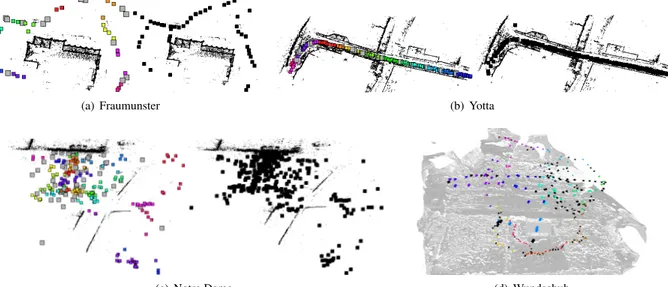
For a qualitative evaluation of the selection method, Fig-ure8shows cluster subdivisions and removed cameras af-ter selection for all datasets, highlighting the regularity of removed cameras. The good coverage properties of our method are also confirmed by a visual analysis of 3D re-constructions: in Figure9the 3D models obtained by using the full image set and our subset are nearly identical.

5. Conclusions

In this work we presented an approach for joint camera clustering and selection, in order to improve Multi-View-Stereo (MVS) scalability.

Two novel methods are introduced. First, we exploit Leveraged Affinity Propagation for clustering, extending the original algorithm to manage cluster and overlaps con-straints. The resulting clusters and diverse overlaps are reg-ular and well-defined, comparing favorably with other state-of-the-art methods [6,15]. Second, we introduce an Integer Linear Programming formulation for view selection. The ILP model treats cameras as binary variables and jointly handles all necessary constraints finding a global solution.

The two methods are combined and it is shown that the final set of clustered and selected cameras ensures a nearly-perfect coverage of the 3D scene and leads to large speedup factors (up to 8x, without parallel processing) compared to MVS reconstructions computed on the full image set.

As future work, we plan to reason about regions of in-terest within the images rather than always considering the full images during selection.

References

[1] S. Agarwala, Y. Furukawaa, N. Snavely, I. Simon, B. Cur-less, S. M. Seitz, and R. Szeliski. Building rome in a day. Commmunications of ACM, 54(10), 2011.1

[2] C. Bron and J. Kerbosch. Algorithm 457: finding all cliques of an undirected graph. Communications of the ACM, 16(9):575–577, 1973.5

[3] D. Crandall, A. Owens, N. Snavely, and D. Huttenlocher. Discrete-continuous optimization for large-scale structure from motion. In CVPR, pages 3001–3008. IEEE, 2011.2

[4] J.-M. Frahm, P. Georgel, D. Gallup, T. Johnson, R. Ragu-ram, C. Wu, Y.-H. Jen, E. Dunn, B. Clipp, S. Lazebnik, and M. Pollefeys. Building rome on a cloudless day. In ECCV. 2010.1

[5] B. J. Frey and D. Dueck. Clustering by passing messages between data points. science, 315(5814):972–976, 2007. 1,

2,4

[6] Y. Furukawa, B. Curless, S. M. Seitz, and R. Szeliski. To-wards internet-scale multi-view stereo. In CVPR, 2010.1,2,

3,6,7

[7] Y. Furukawa and J. Ponce. Accurate, dense, and robust multi-view stereopsis. In CVPR, 2007.1,6

[8] D. Gallup, J.-M. Frahm, P. Mordohai, and M. Pollefeys. Variable baseline/resolution stereo. In CVPR, 2008.1,2

[9] M. Goesele, N. Snavely, B. Curless, H. Hoppe, and S. Seitz. Multi-view stereo for community photo collections. In CVPR, 2007.1,2

[10] C. Hoppe, A. Wendel, S. Zollmann, K. Pirker, A. Irschara, H. Bischof, and S. Kluckner. Photogrammetric Camera Net-work Design for Micro Aerial Vehicles. In CVWW, 2012.

6

[11] A. Hornung, B. Zeng, and L. Kobbelt. Image selection for improved multi-view stereo. In CVPR, 2008.2

[12] http://lpsolve.sourceforge.net/.7

[13] A. Ladikos, S. Ilic, and N. Navab. Spectral camera cluster-ing. In ICCV, 2009.2

[14] X. Li, C. Wu, C. Zach, S. Lazebnik, and J.-M. Frahm. Mod-eling and recognition of landmark image collections using iconic scene graphs. In ECCV, pages 427–440. Springer, 2008.2

[15] M. Mauro, H. Riemenschneider, L. Van Gool, and R. Leonardi. Overlapping camera clustering through dom-inant sets for scalable 3d reconstruction. In BMVC, 2013.1,

2,3,4,6,7

[16] M. Mauro, H. Riemenschneider, L. Van Gool, A. Signoroni, and R. Leonardi. A unified framework for content-aware view selection and planning through view importance. In BMVC, 2014.5

[17] K. Mikolajczyk, T. Tuytelaars, C. Schmid, A. Zisserman, J. Matas, F. Schaffalitzky, T. Kadir, and L. Van Gool. A

(a) Fraumunster (b) Yotta

(c) Notre Dame (d) Wundschuh

Figure 8. Selection results on the four datasets. Removed cameras in black.

(a) Fraumunster (b) NotreDame

(c) Yotta (d) Wundshcuh

Figure 9. Comparison of reconstruction results obtained on the four datasets when using the full set (left) and the selected set (right). comparison of affine region detectors. IJCV, 65(1-2):43–72,

2005.3

[18] M. Pavan and M. Pelillo. Dominant sets and pairwise cluster-ing. Pattern Analysis and Machine Intelligence, IEEE Trans-actions on, 29(1):167–172, 2007.2

[19] H. Riemenschneider, A. Bodis-Szomoru, J. Weissenberg, and L. Van Gool. Learning Where To Classify In Multi-View Semantic Segmentation. In ECCV, 2014.2

[20] S. Seitz, B. Curless, J. Diebel, D. Scharstein, and R. Szeliski. A comparison and evaluation of multi-view stereo recon-struction algorithms. In CVPR, 2006.1

[21] S. Sengupta, P. Sturgess, L. Ladicky, and P. Torr. Automatic Dense Visual Semantic Mapping from Street-Level Imagery. In IROS, 2012.6

[22] E. Shtrom, G. Leifman, and A. Tal. Saliency detection in large point sets. In ICCV, 2013.5

[23] N. Snavely, S. Seitz, and R. Szeliski. Modeling the World from Internet Photo Collections. IJCV, 80(2):189–210, 2007.6

[24] N. Snavely, S. M. Seitz, and R. Szeliski. Skeletal graphs for efficient structure from motion. In CVPR, volume 1, page 2, 2008.2

[25] C. Strecha, W. von Hansen, L. Van Gool, P. Fua, and U. Thoennessen. On benchmarking camera calibration and multi-view stereo for high resolution imagery. In CVPR, 2008.1

[26] D. Tingdahl and L. Van Gool. A public system for image based 3d model generation. In Computer Vi-sion/Computer Graphics Collaboration Techniques, pages 262–273. Springer, 2011.1,2