Calibration of Parallel Kinematic Machines: theory and applications

Calibration of Parallel Kinematic Machines:

Theory and Applications

Giovanni Legnani

1

_{, Diego Tosi}

1

_{, Riccardo Adamini}

1

_{, Irene Fassi}

2

1

_{Dip. Ing. Meccanica -- Università di Brescia Via Branze 38, 25123 Brescia -- Italy}

giovanni.legnani@ing.unibs.it

2

_{ITIA-CNR Institute of Industrial Technology and Automation,}

National Research Council V.le Lombardia 20/A 20131 Milano - Italy

1. Introduction

As already stated in the chapter addressing the calibration of serial manipulators, kinematic calibration is a procedure for the identification and the consequent compensation of the geometrical pose errors of a robot. This chapter extends the discussion to Parallel Manipulators (also called PKM Parallel Kinematic Machines). As described in the following (Section 2) this extension is not obvious but requires special care.

Although for serial manipulators some procedures for the calibration based on automatic generation of a MCPC (Minimum Complete Parametrically Continuos) model exist, for PKMs only methodologies for individual manipulators have been proposed but a general strategy has not been presented since now. A few examples of the numerous approaches for the calibration of individual PKMs are proposed in (Parenti-Castelli & Di Gregorio, 1995), (Jokiel et al., 2000) for direct calibration and (Neugebauer et al., 1999), (Smollett, 1996) for indirect or self calibration techniques. This paper makes one significant step integrating available results with new ones and reordering them in simple rules that can be automatically applied to any PKM with general kinematic chains. In all the cases a MCPC kinematic model for geometrical calibration is automatically obtained.

In Section 2 the main features of PKMs calibration is pointed out and the total number of the necessary parameters is determined; this is an original contribution. In Sections 3 and 4 two novel approaches for the generation of a MCPC model are described. Sections 5 and 6 are dedicated to the analysis of the singular cases and to the procedure for the elimination of the redundant parameters respectively; actual cases are discussed. Section 7 presents several examples of application of the two proposed procedures to many existing PKMs. Section 8 eventually draws the conclusions.

Note: in this chapter it is assumed that the reader has already familiarised himself with the notation

and the basic concepts of calibration described in the chapter devoted to serial manipulators.

2. PKMs Calibration

2.1 Differences with respect to serial robots

The identification of the parameter set to be utilized for parallel manipulators can be performed generalizing the methodology adopted for the serial ones. However some remarkable differences must be taken into account, namely:

Source: Industrial Robotics: Programming, Simulation and Applicationl, ISBN 3-86611-286-6, pp. 702, ARS/plV, Germany, December 2006, Edited by: Low Kin Huat

Open

Access

Database

• most of the joints are ‘unsensed’, that is the joint motion is not measured by a sensor; • PKMs make use of multi-degree of freedom joints (cylindrical, spherical);

• some links have more than two joints;

• links form one or more closed kinematic loops;

• PKMs can be calibrated by ‘internal calibration‘ which does not require an absolute external measuring system.

Internal calibration (also called indirect or self calibration) is performed using the measure of extra-sensors monitoring the motion of non actuated joints and comparing the sensor readings with the values predicted using the nominal manipulator kinematics (Parenti-Castelli & Di Gregorio, 1995), (Ziegert et al., 1999), (Weck et al, 1999). In these cases, some of the manipulator parameters cannot be identified and just a partial robot calibration can be performed. A typical full internal calibration is able to identify all the ‘internal parameters’ (relative position of the joints, joints offsets) but not the location of the arbitrary ‘user’ frames of the fixed and of the mobile bases (6 parameters for the base and 6 for the gripper).

External calibration (also called direct calibration) mainly consists in calibrating the pose of the frame attached to the mobile base with respect to that of the fixed base, and it is similar to the calibration of serial manipulators (Neugebauer et al., 1999), (Smollett, 1996). To perform it, it is necessary to measure the 6 absolute coordinates (3 translations and 3 rotations) of the mobile base. When the instrumentation measures less than 6 coordinates (e.g. when calibration is performed using a double ball bar - DBB), some of the robot parameters cannot be identified and a proper complete external calibration is not possible.

2.2. Identification of the number of the parameters

The number of the parameters necessary to describe a PKM can be very high (e.g. up to 138 for a 6 d.o.f. Stewart-Gough platform). However with standard geometrical dimension of the links, the effect of some of them is usually small and so the corresponding parameters can be neglected. A complete discussion of this ‘reduction’ is outside the scope of this paper which is devoted to identify all the parameters theoretically necessary. However some of the most common situations will be mentioned in Sections 5.2, 6.2 and 7.8.

The first result that should be achieved is the identification of the number of the parameters necessary to construct a MCPC model.

R revolute joint P prismatic joint SS number of singular links

S spherical joint C cylindrical joint F number of reference frames

L number of kin. loops Ji i-th joint E number of encoder (or position sensors)

Table 1 Symbols and abbreviations.

For convenience we report the formula that gives the total number N of the parameters for a generic serial robot

6 2 4 = R+ P+

N (1)

while the number of the internal ones is

6 2 4 = 12 =N− R+ P− Ni (2)

In literature, the only available general result for PKMs is due to Vischer (Visher, 1996) who suggests to generalize Eq.s (1) and (2) as

1) 6( 6 3 = R+P+SS+E+ L+ F− N (3)

where SS is the number of the links composed simply by two spherical joints connected by a rod, E is the number of the encoders (or of the joint sensors), L is the number of the independent kinematic loops and F is the number of the arbitrary reference frames. However Vischer does not give a proof of Eq. (3) but simply states that ‘this equation has been empirically tested on several examples and seems to be valid...’. However some cases are not included and in the following we prove that the correct equation is

1) 6( 6 2 3 = R+P+ C+SI+E+ L+ F− N (4)

where C is the number of cylindrical joints and SI is the number of ‘singular’ links which include the SS links with SI=+1 (Section 5.1) and the SPS legs with SI=−1 (Section 5.2). As proved in the following, spherical joints do not require any parameter and their number is not present in Eq. (4).

Eq. (4) which works both for serial and parallel manipulators can be explained generalizing the Eq. (1) and Eq. (2) given for serial robots. First of all, in the case of serial manipulators we get SS=0, E=R+P, L=0 and F=2 for external calibration while F=0 for internal calibration and so Eq. (3) reduces to Eq.s (1) and (2).

Moreover it is evident that, after choosing an absolute reference frame, each further ‘user’ frame needs 6 parameters (3 rotations and 3 translations) to calibrate its pose; this explains the term 6(F−1).

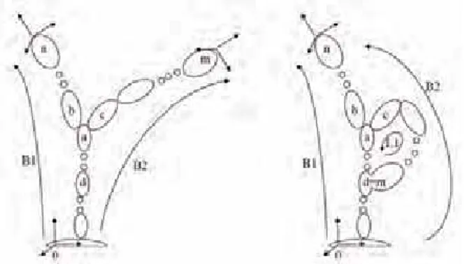
To explain the term L6 we initially consider a serial robot with two ‘branches’ (Fig. 1 left). Its calibration can be performed considering two kinematic chains 1B and 2B from the base frame to the two gripper frames (Khalil et a., 1991). Each joint requires the usual number of parameters, however since we have two grippers the total number of external parameters is incremented by 6 and Eq. (1) is transformed as N=6+6+4R+2P. If now we ‘weld’ link

m

to link d , the number of the parameters is clearly unchanged because the parameters describing the links geometry are still the same and the 6 parameters just added are used to describe the location of the ‘welding’ between the links d− . We conclude that m for each closed loop we add 6 parameters to Eq. (1).

Fig. 1. A serial robot with two branches (left) and one with a closed loop (right).

As a further step we remember that for serial manipulators using the ED&H approach one parameter for each link corresponds to the joint variable. Now since in general in the PKMs

most of the joints are unsensed, we must remove one parameters for each of them; so the term 4 +R 2P of Eq. (1) transforms to 3R+P+E (if all the joints are sensed it is E=R+P). A cylindrical joint can be considered as composed by a revolute joint plus a prismatic one so, apparently, it would require 3 +1=4 parameters. However the direction of the two joint axes coincides and so two parameters must be removed; this explains the term C2 .

Universal joints are kinematically equivalent to a sequence of 2 revolute joints, and can be modelled accordingly.

Spherical joints (ball and socket) can be realised with high accuracy and so they can be often considered ideal and their modellisation requires only three coordinates to represent the location of their center. However spherical joints have 3 DOF and are always unsensed and so we must subtract three parameters. As a result we get zero and so S joints do not appear in Eq. (4). The explication of term SI is more complex and will be analysed in Section 5. At the moment we just observe that for SS links it is evident that the rod length has to be counted as parameter. We also observe that PKMs with SS links hold internal degrees of freedom because the rods can freely rotate about their axes. Other ‘singular links’ will be analyzed in Section 5.

2.3 Comparison between different approaches

By extending the discussion given for serial manipulators in the first part of the work it follows that, since generally in any PKM there are unsensed joints, the Incremental approach will produce a model which is not minimum. It is so necessary to refer to the ED&H or to the Modified Incremental ones.

The adoption of ED&H approaches has the good point that the joint variables are explicitly present in the model and it is then easy to eliminate the joint offsets of the unsensed joints. However it is necessary to define new rules to fix the frames onto the links to take into account the presence of S and C joints. Some manipulators present singular cases that must be treated in a special way. They may result in the temporary insertion of redundant parameters to be removed in a second time.

On the other side, with the modified incremental approach it is nearly impossible to develop an algorithm for a general PKM that automatically generates a ‘minimum’ model. It is always necessary to generate a model that contains some redundancy and then eliminate them. This operation can be difficult because the jacobian to be analyzed could be quite large since it has a number of columns equal to the number of the parameters and a number of rows equal to the number of the scalar equations (6(L+ F−1)). As already mentioned a Stewart-Gough PKM with URPU legs has 138 parameters and 5 loops producing a jacobian matrix with 36 rows and 138 columns. However this procedure can be automatized and it is sometime possible to work just on a part of the jacobian as explained for the serial robots in the relative chapter and extended to PKMs in Section 6 of this chapter.

3. An Extended D&H Approach for PKMs

3.1 Description of the procedure

The extension to PKMs of the ED&H methodology proposed for serial manipulators is based on the adoption of the multi frame approach (Section 9) which requires the definition on each link (fixed and mobile bases included) of a frame for each joint. One of them will be called ‘intrinsic‘ frame of the link and the other ‘auxiliary‘ frames of the joint. The univocal definition of the intrinsic frame, discussed further on, allows to verify once for all the minimality of the parameters used to describe the relative position of the joint auxiliary frames.

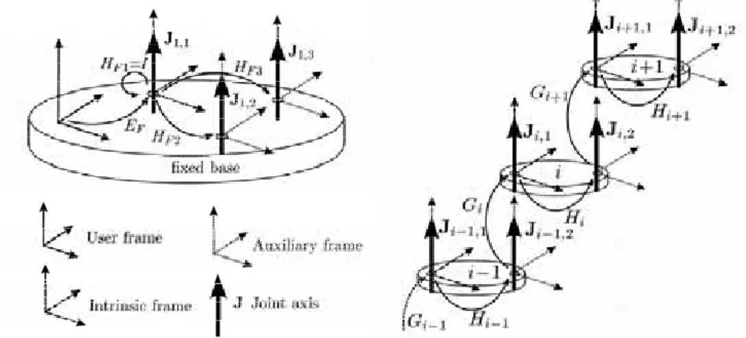
We indicate with H the matrices that describe the relative position of two frames embedded onto the same link (link transformation) while matrices G describe the relative location of the frames of two links connected by a joint, that is the assembly an the motion of the joint (Fig. 2 and Fig. 3). The matrices H depend on some geometrical parameters called ‘link parameters‘.

The fixed base and the mobile base have an extra ‘user‘ frame. Their pose with respect to the intrinsic frame will be described by matrices E (fixed base) and _F E_M (mobile base).

A PKM with F user frames and L loops requires L+ F−1 kinematics equations: one for each (closed) loop and one for each user (gripper) frame to represent its pose with respect to the fixed one (‘branch’ or ‘open loop’). For each PKM different alternative choices are possible. For example for the PKM of Fig. 1-right three alternatives are possible: one equation for each of the two branches 1B and 2B , or one equation for loop 1L and one equation for one of the two branches ( 1B or 2B ).

Fig. 2. Transformation matrices between user, intrinsic and joint auxiliary frames for the fixed base (example of a PKM with 3 legs). The auxiliary frame of the first leg coincides with the intrinsic frame and so HF1=I. The matrices of the mobile base are similar.

Fig. 3. Transformation matrices between the frames of three consecutive links with 2 joints. The pose of the joint frame J_i+1,2 with respect to J_i−1,1 is obtained as M =Hi₋₁GiHiGi₊₁Hi₊₁.

The kinematic equations are obtained in matrix form by multiplying all the matrices that describe the relative position of the frames encountered by travelling along the considered branches or loops. For each branch we follow this path:

• Start from the absolute user frame and move to the intrinsic reference frame of the fixed base. This transformation is described by the matrix E_F

• Move to the joint frame of the first joint of the branch (matrix H ).F

• Move to the joint frame embedded on the next link (matrix G ). • Move to the last joint frame of the same link (matrix H ). • Repeat the two previous steps until the last link (mobile base). • Move to the user frame of the mobile base (matrix E ).M

When a loop is considered only the joint frames must be considered: • start from the last joint frame of an arbitrary link of the loop. • move to the first joint frame of the next link (matrix G ). • move to the last joint frame of the same link (matrix H ).

• repeat the two previous steps for all the joints of the kinematic loop. The kinematics equations result as:

M Mk nk k k k k Fk F k E H G H G H G H E

M = _{1 1 2 2} ! for the k-th branch k=1,b

mj j j jH G H

G

I= _{1 1 2} ! for the j-th loop j=1,A (5)

1

= + −

+ L F

b A

where I denotes the identity matrix, M is the pose of the gripper at the end of the k k -th

branch, n is the number of the joints encountered on the branch and m is the number of the links composing the j -th loop. b and A are the number of equations for branches and loops (b≥ F−1, A≤L). Subscripts k and

j

will be often omitted for simplicity. Matrices

F

E and E are identical for all the branches. _M

A complete set of rules to assign the location of the frames is given in the following Sections which also discuss the singular cases.

3.2 Definition of the intrinsic frames

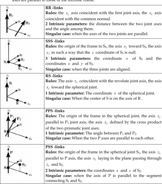
As already mentioned, on each link it is necessary to fix an ‘intrinsic frame’. The procedure is conceptually equivalent to that adopted for serial manipulators when frames are embedded on links with the D&H approach. The rules used for the positioning of the intrinsic frame avoid the use of redundant parameters. However, those rules must be generalized to consider also cylindrical and spherical joints. The necessary rules are summarized in Table 2 where the type of the link is identified by the group of its joints used to define the intrinsic frame. Table 2 also presents the intrinsic parameters of the links and the condition of singularity that may happen.

In links having several joints, different choices may sometimes be performed to define the intrinsic frame all resulting in a different but equivalent model. For example, in a link with two revolute joints (R) and a spherical one (S), it is possible to adopt the rules for RR -links or that for RS ones. Some considerations must be done. C joints are not explicitly mentioned because they follow the rules given for the R ones. Moreover PS -joints (spherical joints that move on a straight line) also follows the rules of R joints; no parameters are defined in this case for the prismatic joint offset which is assumed to be null. Finally, if a link is composed by two R or

Cparallel joints only, the Hayati representation has to be adopted. When on one link more joints of the same type are present, they can be arbitrary numbered.

The geometry of some links does not allow a complete automatic definition of the intrinsic frame (‘singular cases’). In these cases, some parameters that define the origin position and/or the attitude of the intrinsic frame can be partially freely assigned and they do not enter in the calibration model. All these singular cases are described in Table 3.

3.3 Definition of the auxiliary joint frames ( H matrices)

For each joint of each link, an auxiliary joint frame must be defined following some rules dependent on the joint type:

• R and C joints: the axis

z

is chosen coincident to the joint axis. The axis

x

is chosen to lay on the common normal to the joint axis and one axis (generally

_z

) of the intrinsic frame which is not parallel to it.

• P joints: the axis

z

is parallel to the joint axis. The axis

_x

is defined as for revolute joints. Like the standard D&H links the origin of the frame can be freely translated so that in the assembly configuration it coincides with the origin of the frame associated to the first revolute or spherical joint which follows it in the kinematic chain.

• S joints: the origin of the frame coincides with the center of the joints and the frame axes are parallel to those of the intrinsic frame.

RR -links

Rules: the z axis coincident with the first joint axis, the _i x axis _i coincident with the common normal.

2 Intrinsic parameters: the distance between the two joint axes and the angle among them.

Singular case: when the axes of the two joints are parallel.

SSS -links

Rules: the origin of the frame in S1, the axis x toward S_i 2, the axis

i

y in such a way that the z coordinate of S3 is null.

3 Intrinsic parameters: the coordinate x of S2 and the coordinates x and y of S3.

Singular case: when the three joints are aligned.

RS -links

Rules: The axis z coincident with the revolute joint axis, the axis i i

x toward the spherical joint.

1 Intrinsic parameter: The coordinate x of the spherical joint.

Singular case: When the center of S is on the axis of R .

PPS -links

Rules: The origin of the frame in the spherical joint, the axis z_i parallel to P1 joint axis, the axis x defined by the cross product _i of the two prismatic joint axes.

1 Intrinsic parameter: The angle between P1 and P2.

Singular case: When the two P axes are parallel to each other.

PSS -links

Rules: the origin of the frame in the spherical joint S1, the axis z_i parallel to P axis, the axis x laying in the plane passing through _i

i

z and S2.

2 Intrinsic parameters: the coordinates x and z of S2.

Singular case: when the axis of P is parallel to the segment connecting S1 and S2.

SS -links

Rules: the origin of the frame in S1, the axis

z

toward S2, the orientation of x and y axis arbitrary but orthogonal to the

z

axis.

1 Intrinsic parameter: the coordinate z of S2.

1 Free parameter: the rotation around

z

axis.

PS -links

Rules: the origin of the frame in S, the axis z parallel to P , the orientation of x and y axis arbitrary but orthogonal to z axis.

None intrinsic parameter

1 Free parameter: the rotation around z axis.

RP -links

Rules: the axis z coincident to the R joint axis, the axis

x

in such a way that the P axis is parallel to the yz plane.

1 Intrinsic parameter: the angle between the joint axes.

1 Free parameter: the translation along z.

PP -links

Rules: the axis z parallel to the P1 joint axis, the axis x in such a way that the P2 axis is parallel to the yz plane ( =x P2× P1).

1 Intrinsic parameter: the angle between the joint axes.

3 Free parameters: the translations along x , y and

z

. Table 3. Rules to position the intrinsic frames on a link with free parameters (singular cases). In all the mentioned cases a constant matrix H (the ‘link matrix’) can be built to represent the location of the auxiliary joint frame with respect to the intrinsic one. This matrix has generally the form of D&H-like standard matrices defined by two translations and two rotations. However for

Sjoints three translations are required. As usual when a prismatic joint is present, its location can be arbitrary assigned and so two redundant parameters are inserted.

During the construction of the matrices H for the joints which have been involved in the definition of the intrinsic frame some parameters have necessarily a constant null value and so they are not inserted in the calibration parameter set Λ . For instance in a link with ns>3 spherical joints labelled

s n

S S

S1, 2,", where the intrinsic frame is assigned with the rules of Table 2, the matrices describing the joint frames locations are:

) , ( ) , ( = ) , ( = = 2 2 3 3 3 1 I H T xx H T xx T y y H s i i i i T x x T y y T zz i n H = ( , ) ( , ) ( , ) =4!

where I is the identity matrix. So we need 3(ns−2) parameters to describe their relative position.

As a further example, in a link with 3 revolute joints R1, R2and R3and a spherical one (labelled 4), assuming that the intrinsic frame have been defined using the revolute joints R1 and R2, we get

) , ( ) , ( ) , ( ) , ( = ) , ( ) , ( = = 2 2 2 3 3 3 3 3 1 I H T xl Rxϕ H T zh Rzθ T xl Rxϕ H ) , ( ) , ( ) , ( = 4 4 4 4 T x x T y y T zz H

Note: for all the link types the frame of the first joint coincides with the intrinsic one and so I

H =1 .

3.4 Joint assembly and joint motions ( G matrices)

If all the mentioned joint frames are defined with the given rules, R, C and P joints axes will coincide with the

z

axes of a frame (intrinsic or auxiliary). The relative assembly and motion of contiguous links can be then described by the ‘joint matrices’ G defined as_i

joints for ) , , , , , ( = joints and , for ) , ( ) , ( = 2 1 S C R P + + i i i i i i i q q q z y x R G z R c z T G γ

where

c

_i and γ_i are joint coordinates or assembly condition in dependence of the joint type (Table. 10 in Section 9) while R(x,y,z,qi,qi+1,qi+2) is often represented by the product of three elementary rotations around orthogonal axes.

3.5 Parameters set for the ED&H approach

The complete set of parameters to be included in the MCPC calibration model is composed by increments of all the parameters describing the matrices

E

, G ,

H

necessary to write the

1 − + F

L kinematics equations (Eq. (5)).

From the set of the parameters must be removed the offsets of the unsensed joints and the redundant parameters due to the P joints or the singular SS links. The elimination can be performed applying the methodology described for the serial robots in relative chapter and adapted to PKMs in Section 6.

When the external calibration is to be performed it is not necessary to define the intrinsic frame of the fixed and of the mobile base. If this alternative is chosen, a joint frame must be defined for each joint connected to the base and their position is assigned with respect to the user frame.

4. Modified Incremental Approach

When an external calibration is required, the identification of the parameters set to form the calibration model can be performed upgrading the modified incremental approach developed for the serial manipulators in the first part of this work.

It is possible to define on each link a number of frames equals to the number of its joints minus one (n_j−1) and then representing the nominal kinematics of the PKM by a suitable number of matrix equations as already indicated by Eq. (5)

1 = 1, = loop each for = 1, = branch each for = 2 1 2 1 0 − + + L F b j A A A I b k A A A A M mj j j nk k k k k A A ! ! (6)

These matrix equations are equivalent to Eq. (5) with A0k =EFHFk, A =ik GikHik and M

nk nk nk G H E

A = . Eq.s (6) are then updated adding the matrices B describing errors in _i the joint location, matrices E_F′ and EM′ describing the errors in the location of the frames

of the fixed and of the mobile frames and the matrices D describing the offset in the joint _i coordinates. Assuming that the intrinsic frame is attached to the first joint of each link encountered travelling from the base to the gripper we get

loop each for = branch each for = 2 2 2 1 1 1 1 1 1 2 2 1 1 1 0 0 m m m M n n n n n n F B A D B A D B A D I E A B D B A D A D B A D B A E M ! ! _{− − − ′} ′ ₍₇₎

where the subscripts k and j have been omitted for simplicity. If the intrinsic frame is attached to the second joint of the link or for i=n the product A_iB_i commutes to B_iA_i. Matrices EF′ and EM′ are identical for all the branches.

Assuming that the frames are created in such a way that the axes of R, P and C joints coincide with

z

axes, the matrices B ,_i E′ and F E′ are as followsM

) , ( ) , ( ) , ( ) , ( = i i i i i R x R y T x a T y b B Δα Δβ Δ Δ if Ji+1=R or C ) , ( ) , ( = i i i R x a R y b B Δ Δ if Ji+1=P ) , ( ) , ( ) , ( = i i i i T x a T y b T z c B Δ Δ Δ if Ji+1=S ) , ( ) , ( ) , ( ) , ( ) , ( ) , ( = k k k k k k k T x a T y b T z c R x R y R z E ′ Δ Δ Δ Δα Δβ Δγ base frame k=F,M

and B has the same form but depends on J_n n.

Matrices D assume the following form_i ) , ( = _i i R z q D Δ if Ji=R ) , ( = _i i T z q D Δ if Ji=P ) , ( ) , ( = Δ i Δ i+1 i R z q T z q D if Ji=C ) , ( ) , ( ) , ( = Δ i Δ i+1 Δ i+2 i R x q R y q R z q D if Ji=S

Then the Eq.s (7) are analyzed in order to remove from matrices B the parameters which _i are redundant to the joint offsets of matrices D (Section 6). Finally all the parameters _i describing the joint offsets of the unsensed joints are also removed.

To reduce from the beginning the number of the redundant parameters to be removed, the matrices B can be defined taking in account some concepts developed in the _i ED &H methodology. On each link it is necessary to define the intrinsic and the joints frames, a matrix B is defined for each joint frame but some of its parameter can be immediately i

removed. The parameters removed are those whose value is implicitly fixed to zero by the definition of the intrinsic frame.

For instance in a link with ns>3 spherical joints Si, we get

s i i i i T x a T y b T z c i n B b y T a x T B a x T B I B ! 4 = ) , ( ) , ( ) , ( = ) , ( ) , ( = ) , ( = = 2 2 3 3 3 1 Δ Δ Δ Δ Δ Δ

or in a link with 3 revolute joints (R1, R2and R3) and a spherical one (labelled 4), assuming that the intrinsic frame was defined using the revolute joints R1 and R2, we get:

) , ( ) , ( ) , ( = ) , ( ) , ( ) , ( ) , ( = ) , ( ) , ( = = 4 4 4 4 3 3 3 3 3 2 2 2 1 c z T b y T a x T B x R a x T z R c z T B x R a x T B I B Δ Δ Δ Δ Δ Δ Δ Δ Δ α γ α

Note that for all the links we have B =₁ I (see for analogies Section 3.3).

5. Singular Links

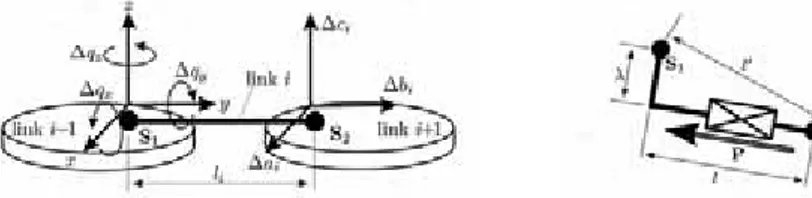
5.1 SS links

The Fig. 4 shows a SS link connecting link i−1 with link i+1. Adopting the modified Incremental approach, among the other parameters, it could be necessary to consider 3 joint offsets Δq_x,i−1, Δq_y,i−1 and Δq_z,i−1 in the joint i−1 and 3 translation parameters Δa_i+1,

1 +

Δbi and Δci+1 in the joint i+1.

An infinitesimal analysis (Section 6) of the error propagation in the kinematic chain gives the following results. The error Δ is equivalent to -ai Δqzi−1li and Δ is equivalent to ci

i xi l

q −1

Δ ; therefore, Δ and ai Δ must be ignored. The joint rotations ci Δqx,i−1, Δqy,i−1, and 1

,−

Δqzi , are to be discharged because the joint is unsensed. And so only Δ survives. The bi

result is that SS -links require just one parameter (the link length); that is SI= +1.

Fig. 4. Redundant parameters on a SS -link. Fig. 5. An actuated SPS leg (λ<<l).

5.2 SPS legs

Fig. 5 represents a simplified scheme of a SPS leg which is often employed in PKMs. According to the general formula (Eq. (4)) such a structure would require two parameters to be described in fact the prismatic link is actuated (P=1, E=1). The two parameters are the link offset λ and the length l . The total link length (the distance between the two spheres) is l′= λ2+l2). However in general it is λ<<l and so l ≅′ l. In these circumstances the parameters λ could be neglected, this is taken into account assigning the value SI= −1 to each SPS leg.

6. Elimination of the Redundant Parameters of PKMs Models

6.1 Analytical reduction

As explained in the chapter devoted to serial manipulators, the relation between the error S

Δ of the gripper pose and the errors in the manipulator geometry Λ can be expressed by means of the jacobian J_Λ

ΔΛ

ΔS=[dx,dy,dz,dα,dβ,dγ]T =JΛ (8)

For PKM, the identification of the redundant parameters to be removed can be performed using the methodology developed for serial robots (see relative chapter). The only difference with the case of serial manipulators is that in general each parameter can be present in more than one of the L+ F−1 kinematic equations (Eq. (7)) and so the redundancy analysis must

be performed analyzing an extended jacobian J formed by the Λ L+ F−1 jacobian J_Λ,k (k=1,L+ F−1) generated from each matrix equation (Eq. (5))

» » » ¼ º « « « ¬ ª Λ Λ ! ! k J J = _,

The matrix JΛ has 6(L+ F−1) rows. The

_i

-th parameter is considered redundant to others if the

i

-th column of J can be expressed as a linear combination of those of the quoted parameters. Λ 6.2 Numerical reduction of the parameters set

The algorithms described in the previous sections lead to a theoretically minimum and complete parametrically continuous set of parameters. For some PKMs, the number of parameters can be very high. However, as already mentioned in the paper, with particular dimensions of the links or when calibration is performed in a limited portion of the working area, some of the parameters may have a very limited effect on the manipulator motion and also considering the measuring errors their value cannot be reliably identified by calibration. We will call them ‘numerically unobservable’ parameters. In other cases two or more parameters may have nearly the same numerical effect on the collected data. In these cases it is not possible to separate their effects and estimate the correct value of all of them. In practice one (or more) of these parameters is considered ‘numerically redundant’. A remarkable example is the link offset λ of SPS legs (Section 5.2).

In general, it is advisable to remove numerically unobservable and redundant parameters from the model to improve the calibration effectiveness because their presence degrades the identification of the numerical value of the parameters especially in presence of measuring noise or in case of not modelled sources of error.

A deep analysis of this topics is outside the scope of this paper but it is worth mentioning how this subject can be addressed. The basic idea is that, as already mentioned, one parameter is redundant if its column of the jacobian matrix can be expressed as linear combination of others. The methodology proposed in Section 6.1 based on an analytical analysis of the jacobian guarantees the elimination of all the redundant parameters. However, in the case of ‘numerically unobservable’ parameters, some columns are theoretically independent to each other but their numerical values is very close to this condition. In this case the elimination algorithm must be based on a numerical analysis of the jacobian and of Eq. (8) evaluated for all the measured poses. One possible approach has been presented in (Tosi & Legnani, 2003). The methodology is based on the analysis of the singular values of the jacobian which assume the meaning of amplification factors of the geometrical errors. A singular value equal to zero means that there is a certain linear combination of parameters which has no effect on the pose of the robot. A singular value whose numerical value is different from zero but lower than a prescribed threshold indicates that there is a parameter (or a group of parameters) that is ‘nearly’ redundant and whose effect is numerically indistinguishable from the others.

Indicating with S the position of the mobile base, with Q the joint positions and with Λ the geometrical parameters we can write

) , ( =F QΛ S ΔΛ ΔΛ Λ ∂ ∂ ≅ ΔSi F =JSi

where F is the direct kinematics and J is the jacobian evaluated in the i-th configuration. _Si The different jacobians evaluated for all the considered m poses as well as the variations in the mobile base pose coordinates can be merged in one global equation

ΔΛ ΔΛ » » » » » ¼ º « « « « « ¬ ª » » » » » ¼ º « « « « « ¬ ª Δ Δ Δ Δ _Stot Sm S S m tot J J J J S S S S = = 2 = 1 2 1 # # (9)

The global jacobian can be splitted in three matrices by Singular Value Decomposition (Press et al. 1993) J_Stot =US_sV converting Eq. (9) in

* * _{= ΔΛ} ΔS_tot S_S with T N T tot T tot U S V S »¼ º «¬ ª_{Δ Δ Δ} ΔΛ ΔΛ ΔΛ Δ Δ * = * = * = λ*₁ λ*₂! λ*

where ΔΛ represents the combined parameters, * ΔS_tot* represents the pose error in the considered configurations and the diagonal matrix Ss contains the singular values of J_Stotthat can

be interpreted as amplification coefficients. If one singular value is lower than a suitable threshold, the corresponding combined parameter can be neglected. The threshold σS depends on the

sensors precision, the manufacturing tolerance and the required final precision. We can define two diagonal weight matrices P containing the maximum acceptable error for the _S

i

-th coordinate of the pose and P containing the maximum expected parameter error for the parameter _Λ λi.

These matrices can be used to normalize the vectors ΔS_tot, and ΔΛ as

ΔΛ Λ Δ Δ Δ − Λ − 1 1 = = P S P Stot _{S tot} (10) Λ

Δ is called ‘scaled’ parameters vector. Merging Eq.s (10) and Eq.(9) it can be found that the proposed procedure based on SVD must be applied to the normalized matrices

Λ Δ Δ Λ − Stot tot Stot S Stot J S P J P J = = 1 (11) In this case, a proper threshold values σS for the singular values depends only on the

dimension of vector Δ . Indeed, the maximum expected parameter error ΛΛ Δ may cause an error on a coordinate

s

_i of the platform smaller than the acceptable one. We can write

2 || || || || = Λ Δ Δ tot ∞ S S σ

where, for a generic vector A , the norms are defined as ||A||∞=max(|ai|) and ||A||2=

¦

ai2.

N ≤ Λ Δ ||2

||

where N is the number of the parameters. From the definition of matrix P we have _S 1

= || ||ΔStot ∞

then, a proper threshold value is

N S= 1 σ R P C SI E L F N Reference 3 1 2 ±1 1 6 6

Stewart-Gough 6[ SPS ] (Jokiel et al., 2000) 0 6 0 0 6 5 2 _{48 (42}♣₎

Stewart-Gough 6[URPU] (Wang et al., 1993) 30 6 0 0 6 5 2 138

3[ CCR ] (Callegari & Tarantini, 2003) 3 0 6 0 3 2 2 40

3[( RP )( RP ) R ] Section 7.4 9 6 0 0 3 2 2 46

6[ PSS ] (Ryu & Rauf, 2001) 0 6 0 6 6 5 2 54

Cheope 3[ P (2 S /2 S )] (Tosi & Legnani, 2003) 0 3 0 6 3 5 2 48

Hexa 6[ RSS ] Fig. 10 6 0 0 6 6 5 2 66

Delta4 3[ R (2 S /2 S )] (Clavel, 1991) 3 0 0 6 3 5 2 54

Table 4. Number of parameters for external calibration (F=2) of some serial or parallel manipulators (Eq. (4)). For Internal calibration subtract 12 parameters (F=0). For extra sensors add the suitable number of parameters. ♣ generally one parameter for each of the 6 SPS leg can be numerically neglected.

7. Examples: Analysis of Some PKMs

This Section analysis some PKMs to clarify the presented methodology for the automatic identification of the parameter set. The discussion refers to Table 4. The manipulators are identified by a code containing the number of legs and the sequence of their joints.

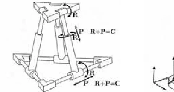
7.1 External calibration of the Stewart-Gough platform with SPS legs

The parameters set of a standard Stewart-Gough platform with spherical joints (Fig. 6) can be identified as follows.

• Fixed base: an ‘user frame’ is created on the fixed base requiring 6 parameters. Then the intrinsic frame is defined using the rules given in Table 2 for SSS -links. The joint frames are created on the spherical joints requiring 0+1+2+3+3+3=12 parameters (Section 3.3). We get a total of 6+12=18 parameters.

• Mobile base: as for the fixed base we get 18 parameters.

• Legs: each leg is composed by two spherical joints connected by a prismatic joint. Each leg then requires P +E=2 parameters.

• Total number of parameters: N = 2*18+6*2 = 48. As a check using Eq. (4) we get R=0, 6

=

h1=h2=0 (nominal values)

Fig. 6 Stewart-Gough platform. The ‘intrinsic frames’ defined on the joints are dashed, the ‘user frames’ are continuous.

Fig. 7 A six-joints URPU leg.

As a control, in this simple case, the same results can be obtained observing that we need 3 coordinates for each spherical joints (their coordinates on the bases) plus the prismatic joint offsets and inclination errors (λ in Fig. 5).

In the common case in which λ<<l, λ can be neglected reducing the number of the parameters by 6 (SI= −6). Total number of parameters ignoring λ is then: N=42. This parameter set has been adopted during the external calibration of several PKMs (e.g., J kiel et al., 2000).

7.2 External calibration of Stewart-Gough platform with URPU legs

Stewart-Gough platforms are usually realized using universal joints in spite of spherical ones, due to their limited performances. Generally, the joints of one base are realized with universal joints plus rotational joints, while the others with bare universal joints (Fig. 7). We assume that also in this case we are interested in representing the mobile base motion with respect to the fixed one in the more general case and so the user base frames can be freely assigned on them. On each of the 6 legs there are 5 not actuated revolute joints and one actuated prismatic joint. Using Eq. (4) it is R=30, P=6, C=0, SI=0, E=6, L=5, F=2 and we get N=138.

Calibrating a so large number of parameters can be a problem but some of them can be neglected because URPU legs are usually realized with intersecting and orthogonal joints axes; referring to Fig. 7, their nominal value is h₁=h₂ =0, (Wang & Masory, 1993), (Wang et al., 1993). In this case, little errors in some of the structural parameters do not affect significantly the mobile base pose (e.g. the relative orientation between joints J −₁ J₂ or

) 6

5 J

J − . As a further example, if the joint inclination changes just a little during PKM operation, errors on h are un-distinguishable from the offset error of the P joint coordinate. _i These parameters are sometimes neglected during external calibration and the URPU leg is modelled as a SPS leg (Patel & Ehmann, 1997). This is not possible when indirect calibration is performed using extra-sensors measuring the leg rotations because, for example, the value of the joint coordinate of J is affected by its orientation with respect to ₂ J .₁

7.3 Stewart-Gough platform calibrated by a double ball bar

Consider the SPS platform of Section 7 and assume that calibration is performed by a double ball bar (DBB) (Ryu & Rauf, 2001). No user frames are defined on the fixed and mobile bases. The number of the parameters is then decreased by 12. Since errors can be also present in the DBB or in its connection to the bases, 8 further parameters are needed (a DBB is cinematically equivalent to an actuated SPS leg). We get: Total number of parameters: N = 48-12+8=44.

If the parameter set is composed by the coordinates of the center of the spherical joints and by 2 parameters for each leg (joint offset and )λ , this would give 56 parameters. To achieve minimality, the number of parameters can be reduced to 44 with a proper choice of the reference frames on the two bases: the origin is located on one sphere S₁, being the

_x

axis directed toward a second sphere S₂, and y axis chosen in such a way that a third sphere

S₃ lies in the x − plane. As a results, the following coordinates error must be neglected y for each base: xΔ , yΔ and zΔ for S₁, Δ and zy Δ for S₂ and zΔ for S₃.

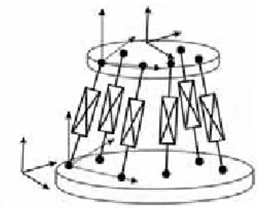
7.4 3[ CCR ] PKM

Fig. 8 represents a 3-dof PKM (Callegari & Tarantini, 2003) witch has three legs with two cylindrical and one revolute joint. If the axes of the cylindrical joints of each leg is orthogonal to the axes of the joints connecting the leg to the fixed and mobile bases, then the motion of the mobile platform is a pure translation. This PKM can be actuated by the prismatic joint located in the legs or those located in the base. We get a total of 40 parameters (Table 2).

The cylindrical pairs can be realized with true C pairs or by a combination of a R and a P joints; in this case it is not possible to assure that their joint axes are exactly parallel and so the number of parameters increases to 46 (see manipulator 3[( RP )( RP ) R ] in Table 4).

Fig. 8 A 3 DOF PKM with CCR. _{Fig. 9. A PKM with PSS legs.}

7.5 6-dof PKM with PSS legs

The analyzed PKM is described in (Ryu & Rauf, 2001). It is similar to the Stewart-Gough platform but the legs have constant length (Figure 9). The mobile base is actuated by moving the ends of the legs on prismatic joints of the fixed base.

For the external calibration 5 parameters are necessary to define the position of the moving end of each leg (4 to define the joint axis, 1 to define the position of the spherical joint on the line), 1 parameter is necessary for each leg (its length), 3 parameters are necessary for each spherical joint on the mobile base. Total number of parameters: N =6*(5+1+3)=54. This number is confirmed by eq. Eq. (4) and Table 4.

If indirect calibration is performed by a DBB, in analogy with what discussed for the Stewart-Gough platform, we get: Total number of parameters: N =54-12+8=50.

If we have only 3 slides each one moving 2 spherical joints we get the Cheope manipulator (Tosi & Legnani, 2003) which has 48 parameters (Section 7.8).

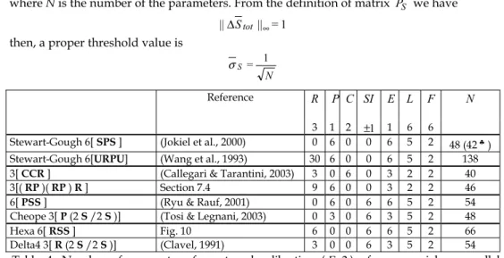
7.6 PKM with RSS legs (Hexa manipulator)

Equations: Let us consider a generic 6[ RSS ] PKM with rotational actuated joints. The

i

-th leg is shown in Fig. 10-left. According to Eq. (4) and to Table 4, the model requires 66 parameters. Adopting an ED&H model, the complete transformation matrix M , describing the position and the orientation of the gripper with respect to the reference frame, comprehensive of all possible geometrical and joint offset error parameters of the

i

-th leg, is (Eq. (5), Fig. 10-right):

M Mi i i i i i Fi F H G H G H G H E E M = ⋅ ⋅ _{1 1} ⋅ _{2 2} ⋅ ₃ ⋅

while for the modified incremental approach we need for each leg

M i i i i i i i i i i F A B D A B D A B B A E E M = ⋅ 0 0 ⋅ 1 1 1 ⋅ 2 2 2 ⋅ 3 3 ⋅

If internal calibration is performed, some error parameters, modelled by matrices B and D , can be neglected, and E_F =E_M =I . For a comparison between the available alternatives see Table 5, Table 6, Table 7 and Table 8.

Internal calibration: An intrinsic frame is defined on the fixed base considering the revolute joints of leg 1 and leg 2 and on the mobile base considering the spherical joints of legs 1, 2 and 3.

Fig. 10. Reference frames and transformation matrices for nominal kinematics on

i

-th leg of a

RSSPKM. The actuator is on the R joint.

Internal Parameters

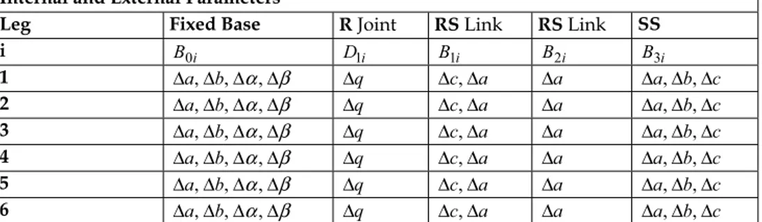
Leg Fixed Base R Joint RS Link RS Link SS

i _{HFi G1i H1i H2i HMi} 1 - Δ ,c Δq Δa Δa -2 Δ ,lΔϕ Δ ,c Δq Δa Δa Δa 3 Δh,Δθ,Δl,Δϕ Δ ,c Δq Δa Δa Δ ,a Δb 4 Δh,Δθ,Δl,Δϕ Δ ,c Δq Δa Δa Δa,Δb,Δc 5 Δh,Δθ,Δl,Δϕ Δ ,c Δq Δa Δa Δa,Δb,Δc 6 Δh,Δθ,Δl,Δϕ Δ ,c Δq Δa Δa Δa,Δb,Δc External Parameters Fixed Base _EF Δa,Δb,Δc,Δ_α,Δ_β,Δ_γ Mobile Base E_M Δa,Δb,Δc,Δα,Δβ,Δγ Table 5. The 66 parameters (54 internal, 12 external) of the RSS PKM (ED&H Model).

Internal and External Parameters

Leg Fixed Base RJoint RSLink RSLink SS

i H_Fi G_1i H_1i H_2i H_Mi 1 Δh,Δθ,Δl,Δϕ Δ ,c Δq Δa Δa Δa,Δb,Δc 2 Δh,Δθ,Δl,Δϕ Δ ,c Δq Δa Δa Δa,Δb,Δc 3 Δh,Δθ,Δl,Δϕ Δ ,c Δq Δa Δa Δa,Δb,Δc 4 Δh,Δθ,Δl,Δϕ Δ ,c Δq Δa Δa Δa,Δb,Δc 5 Δh,Δθ,Δl,Δϕ Δ ,c Δq Δa Δa Δa,Δb,Δc 6 Δh,Δθ,Δl,Δϕ Δ ,c Δq Δa Δa Δa,Δb,Δc

Table 6. The 66 parameters of the RSS PKM (ED&H Model, no intrinsic frames on the fixed and mobile bases).

Internal Parameters

Leg Fixed Base R Joint RS Link RS Link SS

i B_0i D1i B1i B2i B3i 1 - qΔ Δ ,c Δa Δa -2 Δ ,a Δα Δq Δ ,c Δa Δa Δa 3 Δa, bΔ ,Δα,Δβ Δq Δ ,c Δa Δa Δ ,a Δb 4 Δa, bΔ ,Δα,Δβ Δq Δ ,c Δa Δa Δa,Δb,Δc 5 Δa, bΔ ,Δ_α,Δ_β Δq Δ ,c Δa Δa Δa,Δb,Δc 6 Δa, bΔ ,Δα,Δβ Δq Δ ,c Δa Δa Δa,Δb,Δc External Parameters Fixed Base E_F Δa,Δb,Δc,Δα,Δβ,Δγ Mobile Base E_M Δa,Δb,Δc,Δα,Δβ,Δγ

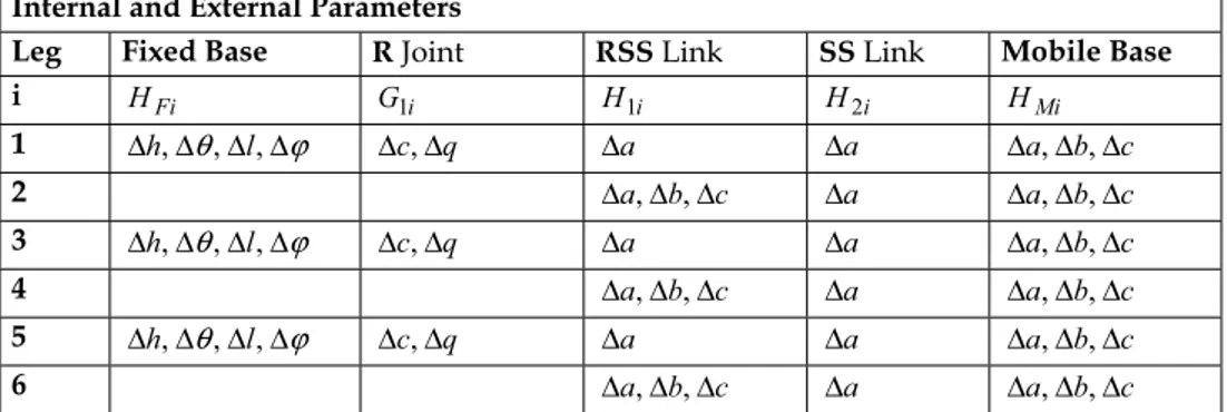
Table 7. The 54 internal and the 12 external parameters of the RSS PKM (Modified Incremental Model).

Internal and External Parameters

Leg Fixed Base R Joint RS Link RS Link SS

i B_0i D_1i B_1i B_2i B_3i 1 Δa, bΔ ,Δα,Δβ Δq Δ ,c Δa Δa Δa,Δb,Δc 2 Δa, bΔ ,Δα,Δβ Δq Δ ,c Δa Δa Δa,Δb,Δc 3 Δa, bΔ ,Δα,Δβ Δq Δ ,c Δa Δa Δa,Δb,Δc 4 Δa, bΔ ,Δα,Δβ Δq Δ ,c Δa Δa Δa,Δb,Δc 5 Δa, bΔ ,Δα,Δβ Δq Δ ,c Δa Δa Δa,Δb,Δc 6 Δa, bΔ ,Δα,Δβ Δq Δ ,c Δa Δa Δa,Δb,Δc Table 8. The 66 parameters of the RSS PKM (ED&H Model, no intrinsic frames on the fixed and mobile bases).

On the RS links an intrinsic frame is constructed with the rules given in Section 3.2. The parameter error aΔ is the link length. Each revolute joint requires the parameter cΔ (translation along the joint axis) and the joint coordinate offset qΔ . On the SS link only the link length error aΔ is to be considered because the spherical joints are not actuated and they do not require any parameter.

External calibration: For external calibration, 12 more parameters are added to describe matrices E and F E containing the errors in the pose of the user frames with respect to the M

intrinsic ones (compare Table 5 and Table 7).

As a second alternative, we can omit to define the intrinsic frames on the two bases and errors of the joints can be defined with respect to the user frame (E_F =E_M =I, Table 6 and Table 8).

7.7 Delta 4 PKM

The delta robot (Clavel, 1991) can be obtained by merging two-by-two the contiguous RS links of the 6[ RSS ] PKM described in Section 7.6. In this case we get R=3, P=0, SI=6,

5 =

L , E=3, C=0, SI= −6 giving a total number of parameters

54 = 1) (2 6 5 5 3 6 0 0 3 * 3 = + + + + + ⋅ + ⋅ −

N for external calibration (Table 9).

Internal and External Parameters

Leg Fixed Base R Joint RSS Link SS Link Mobile Base

i _{HFi G1i H1i H2i HMi} 1 Δh,Δθ,Δl,Δϕ Δ ,c Δq Δa Δa Δa,Δb,Δc 2 Δa,Δb,Δc Δa Δa,Δb,Δc 3 Δh,Δ_θ,Δl,Δ_ϕ Δ ,c Δq Δa Δa Δa,Δb,Δc 4 Δa,Δb,Δc Δa Δa,Δb,Δc 5 Δh,Δθ,Δl,Δϕ Δ ,c Δq Δa Δa Δa,Δb,Δc 6 Δ_a,Δ_b,Δ_c Δa Δa,Δb,Δc

Table 9. The 54 parameters of the Delta4 PKM (ED&H Model, no intrinsic frames on the fixed and on the mobile bases).

7.8 Calibration of the Cheope manipulator

The Cheope manipulator (Fig. 11) has three slides. Each one moves two spherical joints on a linear track. Six spherical joints are located on the mobile platform and 6 rods connect the spherical joints of the platform with those of the slides. The PKM has three translational DOF. Other configurations, not described in this paper, may use the forth slide and an optional seventh rod (Tosi & Legnani, 2003).

As already mentioned in Table 4 Cheope requires 48 parameters for external calibration and 36 for internal. In practice, as mentioned in Section 6.2, many of these parameters may have a limited influence on the manipulator motion and so they can be eliminated from the calibration process. This is quite useful especially in presence of noise in the measures. It is important to note that in many circumstances it is more important to consider the combined effects of some parameters rather than their individual effects. For example in Cheope, the average (and the difference) of the length error of each pair of rods are more significant than the individual length errors. The calibration will then be performed using suitable linear combinations of the parameters rather that using the individual parameters.

The extraction of the reduced set of parameters to be considered as well as the generation of the combined parameters can be automatically performed on the bases of the procedure explained in Section 6.2.

Fig. 11. Photo of the hybrid robot ‘CHEOPE’ and scheme of the parallel kinematic part.

Figure 12 and Figure 13 show the singular values of Cheope respectively for external and internal calibration. For each case three different situations are investigated: a) when both position and rotational errors of the mobile base are important, b) when only position errors are of interest, c) when only rotational errors are considered.

a) S=[x_p y_p z_pθϕψ]T b) S=[x_p y_p z_p]T c) S=[θϕψ]T

Fig. 12. Singular values of matrix JStot in the case of external calibration: (a) complete pose,

(b) position only, (c) rotation only; σS=1/ 48=0.14

a) S=[xp yp zpθϕψ]T b) S=[xp yp zp]T c) S=[θϕψ]T

Fig. 13. Singular values of matrix JStot in the case of internal-calibration: (a) complete pose,

(b) position only, (c) rotation only; σS=1/ 36=0.17.

The dashed line represent the threshold σS , only the parameters associated to the higher

concern, the external calibration requires 30 combined parameters (Figure 12-a) while the internal one can be performed with 24 combined parameters only (Figure 13-a).

The thresholds have been evaluated considering manufacturing errors and joint sensor offsets with a maximum magnitude of 10-5 _{m, required PKM accuracy of 10}-4 _{m, measuring} error of 10-5 _{m for linear sensors and 10}-5 _{rad for the rotational ones.}

8. Conclusions

The paper has presented a complete methodology for the identification of the geometrical parameter set necessary to describe inaccuracy in the kinematic structure of a generic parallel manipulator.

The methodology, that can be applied to any existing PKM, supplies a minimum, complete and parametrically continuous model of the manipulators. It can be applied both to intrinsic (internal) and extrinsic (external) calibration.

The methodology identifies the parameters describing geometric errors of the manipulator, joint offset errors and errors in the external devices used for calibration (e.g. double ball bar). Furthermore, a general formula to determine the total number of necessary parameters has been presented and discussed.

The paper shows how for some manipulators the number of parameters that are theoretically necessary is quite large and a numerical methodology to remove the less significant is mentioned. The final methodology is general and it is an algorithm, this means that it can be automatically applied to any given PKM.

Numerous practical explicative examples are also given.

9. Appendix. D&H Notation: the Multiple Frames Extension

In the first part of this work it has been mentioned how the four D&H parameters of one link represent its geometry, the assembly condition with the previous link and the relative motion with respect to it (joint coordinate). In some situations it is advisable to separate these factors (Sheth & Uicker, 1971) defining a notation with a constant part representing the rigid link and its assembly and a distinct variable part describing (the joint) motion. This is particularly necessary in the calibration of PKMs where there are links with more than two joints. Standard D&H notation for a link with n joints requires the definition of j nj−1

frames attached to it and the so n_j−1 sets of parameters are generated. As an example the case of a ternary link is reported in Fig. 14.

In the quoted example, the frame i is embedded on link A, while frames j and k are placed on link B. The link assembly and the joint motion between the links A - B are represented by the link offsets h and _j h plus the rotations _k θ_j and θ_k. The shape of the link is described by the two lengths l , and j l plus the two twists k ϕj and ϕk and

by the difference between the two rotations θ_B =θ_k−θ_j and of the two link offsets

j k B h h

h = − . To separate the constant and the variable parts Sheth and Uicker propose the adoption of a further frame to be attached on the link B in a free location with the only constrain to have its

z

axis coincident with the joint between the links A - B . In this paper we give rules to assign the location of this frame in a convenient way for calibration purposes (Section 3.2).

Fig. 14 The Denavit and Hartenberg parameters for a ternary link.

In the case of R , P and C joints, the transformation between the frames

i

- j and

i

- k can then be represented as

(

)

(

)

°¯ ° ® ­ ) , ( ) , ( ) , ( ) , ( ) , ( ) , ( = = ) , ( ) , ( ) , ( ) , ( = = k k B B j j Bk j ik j j j j Bj j ij x R l x T h z T z R h z T z R H G M x R l x T h z T z R H G M ϕ θ θ ϕ θ (12) The term Gj=R(z,θj)T(z,hj) is common to both equations and is called ‘joint transformation’.

The product of the other terms is called ‘link transformation’ and will be indicated by H . Each joint has one joint transformation and each link has nj−1 link transformations. If we define on the link B a frame labelled (B) having its axis

z

coincident with the joint between the links A - B and its

x

axis coincident with axis

x

_j, we can interpret the common term G of Eq. (12) as the transformation between frames

i

- B and the others ( H ) as description of the link shape. For simplicity, the frame B is not shown in the figure. The exact interpretation of θ_j and h depends _j on the joint type as shown in Table. 10.

J Type θ_j h_j

R Joint Variable Assembly

P Assembly Joint Variable

C Joint Variable Joint Variable

Table. 10 Meaning of coordinates θ_j and h in the joint matrix _j G of Eq. (12)._j

In this paper, the frame B is called intrinsic frame of the link while j and k are (auxiliary) jointframes. Depending on the number and on the type of the joints of the links, the rules to assign the intrinsic frames must be adapted for calibration purposes in order to avoid singularities and redundancy (Sections 3.2 and 3.3).

10. Acknowledgment

This research work has been partially supported by MIUR grants cofin/prin (Ministero Università e Ricerca, Italia).

11. References

Besnard, S. & Khalil, W. (2001). Identifiable parameters for Parallel Robots kinematic calibration, ICRA 2001, Seoul.

Callegari, M. & Tarantini, M. (2003). Kinematic Analysis of a Novel Translation Platform, Journal of Mechanical Design, Trans. of ASME, Vol. 125, pp. 308-315, June 2003. Clavel, R. (1991) Conception d'un robot parallè le rapide à 4 degrés de liberté, Ph.D. Thesis,

EPFL, Lausanne, Switzerland, 1991.

Denavit, J. & Hartenberg, R. S. (1955). Transactions of ASME Journal of Applyed Mechanics, Vol. 22, pp. 215 - 221, June 1955.

Everett, L. J.; Driels, M. & Mooring, B.W. (1987). Kinematic Modelling for Robot Calibration, Procedeengs of IEEE International Conferenc on Robotics and Automation, Raleig, NC, Vol. 1, pp. 183-189.

Hayati, S. & Mirmirani, M. (1985). Improving the Absolute Positioning Accuracy of robot manipulators, Journal of Robotic Systems, Vol. 2, No. 4, pp. 397-413.

Jokiel, B.; Bieg, L. & Ziegert, J. (2000). Stewart Platform Calibration Using Sequential Determination of Kinematic Parameters, Proceedings of 2000-PKM-IC, pp. 50-56, Ann Arbor, MI, USA.

Khalil, W.; Gautier, M. & Enguehard, C. (1991). Identifiable parameters and optimum configurations for robot calibration, Robotica, Vol. 9, pp. 63-70.

Khalil, W. & Gautier, M. (1991). Calculation of the identifiable parameters for robot calibration, IFAC 91, pp. 888-892.

Legnani, G.; Casolo, F.; Righettini P. & Zappa, B. (1996). A Homogeneous Matrix Approach to 3D Kinematics and Dynamics. Part 1: theory, Part 2: applications, Mechanisms and Machine Theory, Vol. 31, No. 5, pp. 573-605.

Meggiolaro, M. & Dubowsky, S. (2000). An Analytical Method to Eliminate the Redundant Parameters in Robot Calibration, Procedeengs of the International Conference on Robotics and Automation (ICRA '2000), IEEE, San Francisco, CA, USA, pp. 3609-3615. Mooring, B. W.; Roth, Z. S. & Driels M. R. (1991). Fundamentals of manipulator calibration, John

Wiley & Sons, Inc., USA.

Neugebauer, R.; Wieland, F.; Schwaar, M. & Hochmuth, C. (1999). Experiences with a Hexapod-Based Machine Tool, In: Parallel Kinematic Machines: Theoretical Aspects and Industrial Requirements, pp. 313-326, Springer-Verlag, C.R. Bor, L. Molinari-Tosatti, K. S. Smith (Eds).

Omodei, A.; Legnani, G. & Adamini, R, (2001). Calibration of a Measuring Robot: Experimental Results on a 5 DOF Structure, J. Robotic Systems Vol. 18, No. 5, pp. 237-250.

Parenti-Castelli, V. & Di Gregorio, R. (1995). Determination of the actual configuration of the general Stewart platform using only one additional displacement sensor. In: Proc. of ASME Int. Mechanical Engineering Congress & Exposition, Nov. 12-17 1995, San Francisco, CA, USA.

Patel, A. & Ehmann, K. F. (1997). Volumetric Error Analysis of a Stewart Platform Based Machine Tool, Annals of CIRP, Vol. 46, No. 1, pp. 287-290.

Press, W.H.; Flannery, B.P.; Teukolsky, S.A.; Vetterling, W.T. (1993). Numerical Recipes in C/Fortran/Pascal, Cambridge University Press.

Reinhar, G.; Zaeh, M. F. & Bongardt, T. (2004). Compensation of Thermal Errors at Industrial Robots, Production Engineering, Vol. XI, No. 1.