Accepted Manuscript
Assessment of air quality microsensors versus reference methods: The EuNetAir Joint Exercise – Part II
C. Borrego, J. Ginja, M. Coutinho, C. Ribeiro, K. Karatzas, Th Sioumis, N. Katsifarakis, K. Konstantinidis, S. De Vito, E. Esposito, M. Salvato, P. Smith, N. André, P. Gérard, L.A. Francis, N. Castell, P. Schneider, M. Viana, M.C. Minguillón, W. Reimringer, R.P. Otjes, O. von Sicard, R. Pohle, B. Elen, D. Suriano, V. Pfister, M. Prato, S. Dipinto, M. Penza
PII: S1352-2310(18)30543-0
DOI: 10.1016/j.atmosenv.2018.08.028
Reference: AEA 16196
To appear in: Atmospheric Environment Received Date: 27 December 2017 Revised Date: 6 August 2018 Accepted Date: 12 August 2018
Please cite this article as: Borrego, C., Ginja, J., Coutinho, M., Ribeiro, C., Karatzas, K., Sioumis, T., Katsifarakis, N., Konstantinidis, K., De Vito, S., Esposito, E., Salvato, M., Smith, P., André, N., Gérard, P., Francis, L.A., Castell, N., Schneider, P., Viana, M., Minguillón, M.C., Reimringer, W., Otjes, R.P., von Sicard, O., Pohle, R., Elen, B., Suriano, D., Pfister, V., Prato, M., Dipinto, S., Penza, M., Assessment of air quality microsensors versus reference methods: The EuNetAir Joint Exercise – Part II, Atmospheric
Environment (2018), doi: 10.1016/j.atmosenv.2018.08.028.
This is a PDF file of an unedited manuscript that has been accepted for publication. As a service to our customers we are providing this early version of the manuscript. The manuscript will undergo copyediting, typesetting, and review of the resulting proof before it is published in its final form. Please note that during the production process errors may be discovered which could affect the content, and all legal disclaimers that apply to the journal pertain.
M
AN
US
CR
IP
T
AC
CE
PT
ED
1Assessment of Air Quality Microsensors Versus Reference Methods: the EuNetAir
1
Joint Exercise – part II
2
C. Borregoa,b, J. Ginjaa, M. Coutinhoa, C. Ribeiroa, K. Karatzasc, Th. Sioumisc, N. Katsifarakisc,
3
K. Konstantinidisc, S. De Vitod, E. Espositod, M. Salvatod, P. Smithe *, N. Andréf , P. Gérardf, L.
4
A. Francisf, N. Castellg, P. Schneiderg, M. Vianah, M.C. Minguillónh, W. Reimringeri, R.P.
5
Otjesj, O. von Sicardk, R. Pohlek, B. Elenl, D. Surianom, V. Pfisterm, M. Pratom, S. Dipintom, M.
6
Penzam
7
a IDAD – Institute of Environment and Development, Campus Universitário, 3810-193 Aveiro, Portugal
8
b CESAM & Department of Environment and Planning, University of Aveiro, 3810-193 Aveiro, Portugal
9
c Department of Mechanical Engineering, Aristotle University, 54124 Thessaloniki, Greece
10
dSmart Networks and Photovoltaic Division, ENEA, C.R. Portici, 80055 Portici (NA), Italy
11
e Department of Chemistry, University of Cambridge, UK* now at IQFR-CSIC, Calle de Serrano 119, Madrid 28004, Spain
12
fInstitute of Information and Communication Technologies, Université Catholique de Louvain, Belgium
13
gNILU Norwegian Institute for Air Research, Instituttveien 18, 2027 Kjeller, Norway
14
hIDAEA-CSIC, Spanish National Research Council, Jordi Girona 18, 08034 Barcelona, Spain
15
i3S – Sensors, Signal Processing, Systems GmbH, 66121 Saarbruecken, Germany
16
jECN – Energy Research Center of the Netherlands, Petten, Netherlands
17
kSiemens AG, Corporate Technology, Germany
18
lVITO – Vlaamse Instelling voor Technologisch Onderzoek, Mol, Belgium
19
m
ENEA, Laboratory of Functional Materials and Technologies for Sustainable Applications, 72100 Brindisi, Italy
20
Abstract
21
The EuNetAir Joint Exercise focused on the evaluation and assessment of environmental
22
gaseous, particulate matter (PM) and meteorological microsensors versus standard air quality
23
reference methods through an experimental urban air quality monitoring campaign. This work
24
presents the second part of the results, including evaluation of parameter dependencies,
25
measurement uncertainty of sensors and the use of machine learning approaches to improve the
26
abilities and limitations of sensors. The results confirm that the microsensor platforms,
27
supported by post processing and data modelling tools, have considerable potential in new
28
strategies for air quality control. In terms of pollutants, improved correlations were obtained
29
between sensors and reference methods through calibration with machine learning techniques
30 for CO (r2=0.13-0.83), NO2 (r 2 =0.24-0.93), O3 (r 2 =0.22-0.84), PM10 (r2=0.54-0.83), PM2.5 31 (r2=0.33-0.40) and SO2 (r 2
=0.49-0.84). Additionally, the analysis performed suggests the
32
possibility of compliance with the data quality objectives (DQO) defined by the European Air
33
Quality Directive (2008/50/EC) for indicative measurements.
34
35
Keywords: Air quality monitoring; Reference methods; Low-cost microsensors; Experimental campaign; 36
Measurement uncertainty; Machine learning
37
1. Introduction
38
Air pollution is a very significant environmental and social issue. At the same time, it is a
39
complex problem posing multiple challenges in terms of management and mitigation of harmful
40
pollutants. Air pollutants have numerous impacts on health, ecosystems, built environment and
41
climate; they may be transported or formed over long distances, and they may affect large areas.
42
Air pollution continues to affect the health of Europeans, particularly in urban areas. It also has
43
considerable economic impacts; cutting lives short, increasing medical costs and reducing
44
productivity through working days lost across the economy (EEA, 2017; WHO, 2018).
45
According to The World Health Organization (WHO), in 2016, 91% of the world population
M
AN
US
CR
IP
T
AC
CE
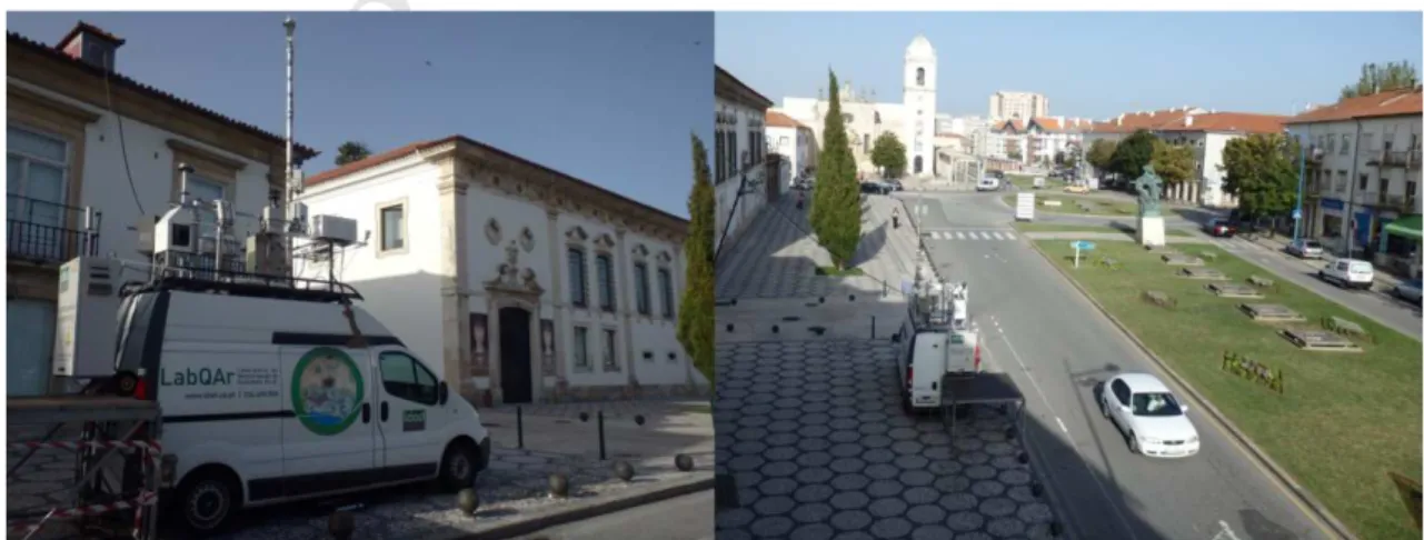
PT
ED
2were living in places where the WHO air quality guidelines limits were not met. Additionally,
47
outdoor air pollution in both cities and rural areas was estimated to cause 4.2 million premature
48
deaths worldwide in 2016 (WHO, 2018).
49
Europe's most problematic pollutants in terms of health are PM, NO2 and ground-level O3.
50
In 2015, about 7 % of the EU-28 urban population was exposed to PM2.5 levels above the EU's
51
annual limit value. Considering the stricter WHO guidelines, approximately 82 % were exposed
52
to levels exceeding the limit values. Exposure to PM2.5 caused the premature death of
53
estimated 428 000 people in 41 European countries in 2014. Regarding NO2, around 9 % of the
54
EU-28 urban population was exposed to levels above the EU's annual limit value and WHO
55
guidelines in 2015. Exposure to NO2 caused the premature death of an estimated 78 000 people
56
in 41 European countries in 2014. For O3 levels, 30 % of the EU-28 urban population was
57
exposed to concentrations above the EU's target value in 2015. Considering the stricter WHO
58
guidelines, approximately 95 % were exposed to levels exceeding the limit value. Exposure to
59
O3 caused the premature death of an estimated 14400 people in Europe in 2014 (EEA, 2017).
60
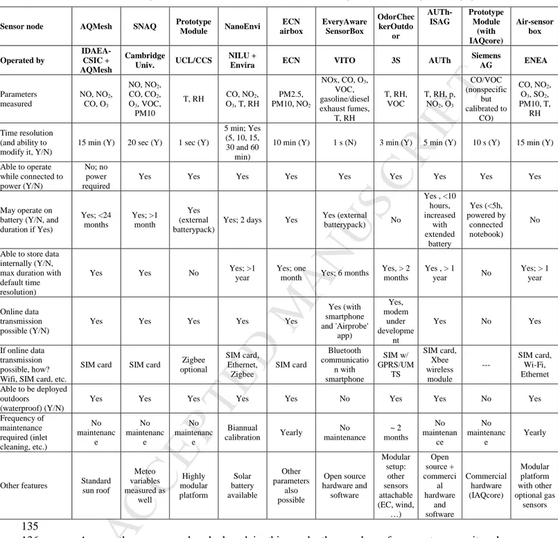
A wide range of adverse effects of ambient air pollution on health has been well
61
documented in multiple studies (Pascal et al., 2013; Wu et al. 2016). By working to reduce air
62
pollution levels, countries can lower the burden of stroke, heart disease, lung cancer, and both
63
chronic and acute respiratory illness, with long-term benefits to the population (WHO, 2018).
64
However, there is significant inequality in exposure to air pollution and related health risks:
65
air pollution combines with other aspects of the social and physical environment to create a
66
disproportionate disease burden in less affluent parts of society. The WHO guidelines address
67
all regions of the world and provide uniform targets for air quality that would protect the vast
68
majority of individuals from the adverse effects on health. More than 80% of the population in
69
the WHO European Region (including the European Union, EU) lives in cities with levels of
70
PM exceeding WHO Air Quality Guidelines. Since even at relatively low concentrations the
71
burden of air pollution on health is significant, effective management of air quality that aims to
72
achieve WHO Air Quality Guidelines levels is necessary to reduce these risks to a minimum.
73
Exposure to air pollutants is largely beyond the control of individuals, requiring action by public
74
authorities at the national, regional and international levels. A multisector approach, engaging
75
transport, housing, energy production and industry is needed to develop and effectively
76
implement long-term policies that reduce the risks of air pollution to health (WHO, 2013).
77
The evaluation of the status of air quality (AQ) is based on ambient air measurements, in
78
conjunction with data on anthropogenic emissions and their trends. Holistic solutions must be
79
found that involve technological development, and structural and behavioural changes. Air
80
quality policies have delivered, and continue to deliver, many improvements. However,
81
substantial challenges remain and considerable impacts on human health and on the
82
environment persist (EEA, 2017).
83
The increasing availability of low cost sensors employing various monitoring principles
84
creates the need to identify which are the most appropriate to be further refined and calibrated.
85
For this purpose, it is necessary to estimate the overall performance of a large number of
86
collocated sensors (Kotsev et al., 2016). This not only calls for the application of standard time
87
series analysis and comparison methods, but also the incorporation of overall measurement
88
profile and behaviour, so that a sensor network may generate reliable AQ data. Calibration
89
methods have been based on sensor intercomparison, as well as on overall sensor network
90
calibration (Jiao et al., 2016) and self-calibration (Fishbain and Moreno-Centeno, 2016). Recent
91
studies indicate that machine learning technologies may significantly improve the performance
92
of air quality sensor nodes reducing the impact of cross-sensitivity issues (Spinelle et al., 2015;
93
De Vito et al., 2018). Most of them however, have been carried out on single systems,
94
developed by the same company or research institutions, limiting the understanding and
95
potential about their general applicability.
M
AN
US
CR
IP
T
AC
CE
PT
ED
3In the first part of this work, the overall results of an intercomparison of AQ microsensors
97
with reference methods during an AQ monitoring campaign in Aveiro, Portugal, were presented
98
(Borrego et al., 2016). The overall performance of the diverse sensors in terms of their statistical
99
metrics and measurement profile indicated significant differences in the results. In terms of
100
pollutants, the following results were observed: O3 (r2: 0.12-0.77), CO (r2: 0.53-0.87) and NO2
101
(r2: 0.02-0.89) with some promising results, but equally sensors showing no correlation with the
102
reference method. For PM (r2: 0.07-0.36) and SO2 (r 2
: 0.09-0.20) the results showed a poor
103
performance with low correlation coefficients between the reference and microsensor
104
measurements.
105
The purpose of this study is to present the second part of the results of the intercomparison
106
campaign in Aveiro for two weeks in October 2014, complementing the analysis performed by
107
Borrego et al. (2016). More specifically, it is intended to (a) understand parameter
108
dependencies, (b) measurement uncertainty of sensors, (c) the use of machine learning
109
approaches to improve the abilities and limitations of sensors, contributing to their calibration
110
and further development.
111
The paper is organized into the following sections: Section 2 gives a description of the
112
experimental campaign and methodology; Section 3 presents the results obtained with the
113
different data analysis strategies; finally, Section 4 provides the conclusions.
114
2. Experimental Design
115
2.1.Characterization of the study site
116
In this exercise, the AQ microsensor systems were installed side-by-side on the IDAD Air
117
Quality Mobile Laboratory (LabQAr), supplied with standard equipment and reference
118
analysers for CO (Infrared photometry), NOx (Chemiluminescence), O3 (Ultraviolet
119
photometry), SO2 (Ultraviolet fluorescence), particulate matter PM10 / PM2.5 (Beta-ray
120
absorption), and meteorological variables (Vaisala WXT520). During the exercise, LabQAr was
121
parked on Avenue Santa Joana, near the Cathedral of Aveiro, in an urban traffic location in
122
Aveiro city centre. The sensors were mainly installed between 2.5 and 3 m above ground on the
123
roof of the mobile laboratory, with the reference meteorological measurements at ~ 5 m on a
124
telescopic mast (Fig. 1).
125
126
Fig. 1. Set-up of the AQ mobile station and micro-sensors during the 1st EuNetAir campaign.
127
2.2.Comparison of technical requirements of the sensor nodes
128
Aside from the performance of the sensor nodes with regard to comparability with
129
reference instruments, discussed in Borrego et al. (2016), the selection of a specific sensor node
130
should also consider a number of technical parameters as well as data quality and uncertainty.
M
AN
US
CR
IP
T
AC
CE
PT
ED
4These include; size, power, connectivity requirements, and number of pollutants monitored
132
(Table 1).
133
Table 1. Technical requirements and features of the sensor nodes evaluated during the Aveiro intercomparison campaign. 134
Sensor node AQMesh SNAQ Prototype
Module NanoEnvi ECN airbox EveryAware SensorBox OdorChec kerOutdo or AUTh-ISAG Prototype Module (with IAQcore) Air-sensor box Operated by IDAEA-CSIC + AQMesh Cambridge Univ. UCL/CCS NILU +
Envira ECN VITO 3S AUTh
Siemens AG ENEA Parameters measured NO, NO2, CO, O3 NO, NO2, CO, CO2, O3, VOC, PM10 T, RH CO, NO2, O3, T, RH PM2.5, PM10, NO2 NOx, CO, O3, VOC, gasoline/diesel exhaust fumes, T, RH T, RH, VOC T, RH, p, NO2, O3 CO/VOC (nonspecific but calibrated to CO) CO, NO2, O3, SO2, PM10, T, RH Time resolution (and ability to modify it, Y/N)
15 min (Y) 20 sec (Y) 1 sec (Y)
5 min; Yes (5, 10, 15, 30 and 60 min)
10 min (Y) 1 s (N) 3 min (Y) 5 min (Y) 10 s (Y) 15 min (Y) Able to operate while connected to power (Y/N) No; no power required
Yes Yes Yes Yes Yes Yes Yes Yes Yes
May operate on battery (Y/N, and duration if Yes) Yes; <24 months Yes; >1 month Yes (external batterypack)
Yes; 2 days Yes Yes (external batterypack) No
Yes , <10 hours, increased with extended battery Yes (<5h, powered by connected notebook) No
Able to store data internally (Y/N, max duration with default time resolution)
Yes Yes No Yes; >1
year
Yes; one
month Yes; 6 months
Yes, > 2 months Yes , > 1 year No Yes; > 1 year Online data transmission possible (Y/N)
Yes Yes Yes Yes Yes
Yes (with smartphone and 'Airprobe' app) Yes, modem under developme nt Yes No Yes If online data transmission possible, how? Wifi, SIM card, etc.
SIM card SIM card Zigbee optional SIM card, Ethernet, Zigbee SIM card Bluetooth communicatio n with smartphone SIM w/ GPRS/UM TS SIM card, Xbee wireless module --- SIM card, Wi-Fi, Ethernet Able to be deployed outdoors (waterproof) (Y/N)
Yes Yes Yes Yes Yes No Yes Yes No Yes
Frequency of maintenance required (inlet cleaning, etc.) No maintenanc e No maintenanc e No maintenanc e Biannual calibration Yearly No maintenance ~ 2 months No maintenan ce No maintenanc e Yearly
Other features Standard sun roof Meteo variables measured as well Highly modular platform Solar battery available Other parameters also possible Open source hardware and software Modular setup: other sensors attachable (EC, wind, …) Open source + commerci al hardware and software Commercial hardware (IAQcore) Modular platform with other optional gas sensors 135
Among the sensor nodes deployed in this work, the number of parameters monitored
136
ranged between one and seven, also covering meteorological variables. Time resolution ranged
137
from 1-second up to 15-minute averages, suggesting different potential applications. For
138
example, the 1-second time resolution of the EveryAware sensor box is well suited to personal
139
exposure, while the 15-minute averages produced by the AQMesh and ENEA nodes would be
140
more representative of ambient pollutant concentrations. However, this does not preclude the
141
different sensor nodes being deployed for the same application, as was the case in this exercise.
142
One of the goals for widespread use of sensor technologies for air quality monitoring is to
143
maximise spatial data coverage (Castell et al., 2013; Schneider et al., 2017), by deploying dense
M
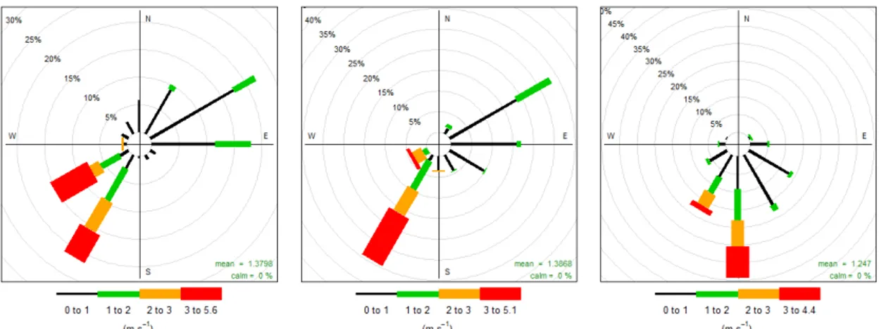
AN
US
CR
IP
T
AC
CE
PT
ED
5networks of sensors, e.g. across urban areas. However, this is not feasible if the nodes present
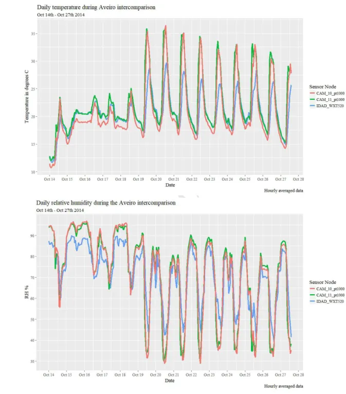
145
limitations with regard to connectivity or power requirements. As shown in the Table 1 most of
146
the nodes (7 out of 8) are able to operate on battery, minimising the need to provide mains
147
power at the measurement locations. Also, all of them are able to transmit data, either directly to
148
“cloud” platforms or through apps on mobile phones. Only one of the nodes requires Wi-Fi
149
access, which is a potentially limiting factor for large scale deployment across urban areas.
150
Finally, 7 out of the 8 nodes may be deployed outdoors (only one of them requiring additional
151
protection to be built), being resistant to weather conditions. The latter requirement would be
152
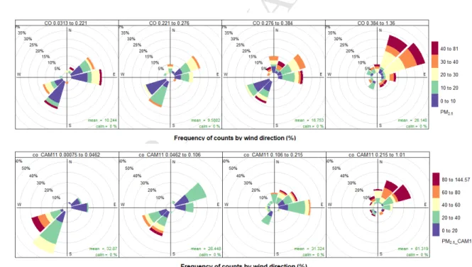
irrelevant when dealing with indoor air quality monitoring.
153
For outdoor air quality monitoring, the frequency of maintenance is a relevant parameter.
154
Whereas most of the nodes require no or limited (yearly) maintenance, one node requires
155
maintenance or calibration every 2-6 months. In terms of operation and data availability,
156
frequent maintenance may be an issue for sensor node selection.
157
2.3.Calibration strategies
158
Some of the installed AQ microsensors output results in concentration units while others
159
provide voltage or frequency data. Therefore, a pre-processing of raw data was necessary to
160
proceed to concentration units. All sensor nodes (with the exception of the Siemens node) have
161
hence been pre-calibrated. Each team was responsible for their own unit conversion, including
162
different calibrations and conversion strategies, depending on the sensors used. Additional
163
information is presented in Supplementary Material (Table S1).
164
The gas sensors used for the AUTh-ISAG node were off-the-shelf metal-oxide sensors that
165
did not undergo a specialized calibration procedure by their manufacturer. In this case it was
166
decided to apply a simple signal correction procedure in order to calibrate the readings received,
167
assuming a linear calibration approach as suggested by Balzano and Nowak (2008).
168
The NanoEnvi node did not undergo a specialized calibration procedure by their
169
manufacturer. The data was not post-processed to correct for temperature and humidity effects
170
or cross-interference with other gases. For the analysis, only the negative concentration values
171
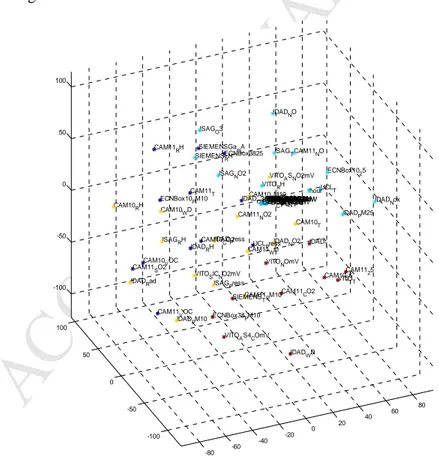
were removed. Negative values were only registered for the NO2 sensors and represented about
172
20% of the total data.
173
The two ECN-Airbox were calibrated before the Aveiro campaign carrying out co-located
174
measurements with reference equipment at an official monitoring station in Amsterdam
175
(NL49014 GGD Vondelpark). The ECN sensors were developed to minimize cross
176
contamination and meteorology interference. For the NO2 sensor this was established by
177
introduction of a differential measurement technique enforced by a pre-processing step prior to
178
the sensor by switching frequently to zero ambient airflow (NO2 removed). Moreover, the
179
sample flow was stabilized by a patented RH delaying cartridge.
180
The AQMesh v 4.0 pods used in this experiment reported NO, NO2, CO and O3
181
concentrations which are the result of a two-stage process, following the AQMesh standard
182
operating procedure (SOP). In the first stage, the AQMesh algorithm (a fixed mathematical
183
formula which does not use machine learning) is applied to the raw data in counts, which are
184
converted to ambient concentration units, along with compensation for various environmental
185
effects upon the sensors, providing precision of measurement. The AQMesh SOP requires that
186
pods are deployed 2 weeks prior to the actual measurements for stabilization and application of
187
scaling using reference data. Given that the logistics did not allow doing so in this field
188
campaign, the calibration via scaling was done in this study using the reference data from the
189
trial period.
190
The EveryAware SensorBox (EA SB) is a portable, low-cost measurement device, which
191
allows measurements of the personal exposure to traffic pollution. The EA SB combines a
M
AN
US
CR
IP
T
AC
CE
PT
ED
6number of low-cost electrochemical and metal oxide sensors to measure concentrations of CO,
193
NO2, gasoline exhaust and diesel exhaust. Furthermore, additional sensors have been added to
194
allow correction for meteorological influences (T and RH sensor) and for cross sensitivities (O3
195
and VOC sensor).
196
The ENEA-Air-Sensor Box used in the Aveiro campaign consisted of commercial low-cost
197
electrochemical sensors for gas (NO2, O3, CO, SO2) detection and commercial cost-effective
198
optical particle counter (OPC) for particulate matter (PM10) detection, including miniaturized
199
sensors for meteorology parameters (T and RH). Before the Aveiro campaign, ENEA calibrated
200
the prototype Airbox by co-located measurements with reference analysers in an official air
201
quality monitoring station at JRC, located in Ispra, Italy.
202
During the Aveiro Intercomparison Exercise, two SNAQ (Sensor Networks for Air Quality)
203
boxes were deployed (hereafter referred to as CAM). Both units utilised Alphasense
204
electrochemical cell (ECC, model B4/BH) for species NO, NO2, O3, CO, SO2 and Total VOC.
205
Measurements of CO2 (SenseAir K30) and particulate matter (University of Hertfordshire
206
CAIR) were also undertaken. The CAM boxes employ Gill WindSonic 2-D sonic anemometers
207
to assist in source attribution. Before deployment, each sensor box was fitted with new
208
Alphasense electrochemical cells. Throughout the campaign and subsequent data analysis, only
209
the raw signal data from the sensors was used, correcting for temperature and humidity effects
210
as per Popoola et al., (2016). In addition to the factory calibration of the ECC sensors, a second
211
calibration was employed based on a comparison of both CAM sensor boxes with reference
212
instruments of the Department of Chemistry in Cambridge.
213
2.4.Data analysis and quality control
214
2.4.1 Meteorological measurements
215
One of the most important benefits of AQ monitoring networks is the ability to pinpoint
216
pollution sources, and account for regional (> 50 km), meso-scale (500 m to 50 km) and
micro-217
scale (< 500 m) influences. This requires suitable meteorological data to support the
218
measurements. Due to the influence of urban topography and traffic at the micro-scale it is
219
beneficial to have meteorological measurements in the same place as the AQ sensors (Popoola
220
et al., 2013). During the Aveiro campaign, principal meteorological variables were measured by
221
the IDAD LabQAr van using a Vaisala WXT 520 weather station (Borrego et al., 2016). The
222
CAM_10 and CAM_11 boxes measured wind speed, wind direction, temperature and humidity,
223
allowing comparison of meteorological variables and source apportionment.
224
2.4.2 Measurement uncertainty
225
The European Air Quality Directive (EU, 2008) defines the Data Quality Objective (DQO)
226
that monitoring methods need to comply with to be used as indicative measurement for
227
regulatory purposes. The DQO is a measure of the acceptable uncertainty for indicative
228
measurements. According to the Directive, allowed uncertainties are 50% for PM10 and PM2.5,
229
30% for O3 and 25% for CO, NOx, NO2 and SO2.
230
To assess the performance of each sensor and of the sensor platform as a whole, the
231
measurement of uncertainty has been calculated following the methodology described in JCGM
232
(2008) and Spinelle et al. (2015). The relative expanded uncertainty was estimated using
233
Equation 1, where indicates the reference measurement, the candidate method (sensor),
234
and are the slope and intercept of the orthogonal regression, respectively, RSS is the sum of
235
squares of the residuals (Equation 2), and is the uncertainty of the reference instrument.
236
Further details on the calculation of the expanded uncertainty can be found in the Guide for the
237
demonstration of equivalence (EC WG, 2010).
M
AN
US
CR
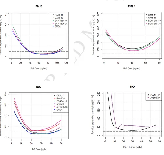
IP
T
AC
CE
PT
ED
7=
!(1) 239 "## = ∑ − − (2) 240
2.4.3 Multidimensional data visualization
241
In order to investigate the behaviour of the AQ nodes in terms of the monitored parameters,
242
it was decided to visualize all meteorological and gaseous data in a way that can reveal
243
dependencies and similarities of patterns; information that can be of value for the node
244
validation and calibration. For this reason, the T-distributed Stochastic Neighbour Embedding
245
(t-SNE) method was employed. This is a relatively new nonlinear mapping technique that is
246
capable of preserving both the local and global structure of a high dimensional dataset (van der
247
Maaten and Hinton, 2008). As multiple parameters (like air pollutant concentrations and
248
meteorological conditions) are produced from the operation of the sensor boxes, it is impossible
249
to simultaneously visualize them and thus investigate possible relationships. The t-SNE method
250
is capable of visualizing this high dimensional feature space in a lower dimensional (2-D or
3-251
D) space. The main characteristic of the method is that the groups or clusters of features (here
252
consisting of AQ nodes and reference measurements) appearing in t-SNE reflect similarities,
253
thus the closer the attributes are to each other forming a group, the more they can be considered
254
as similar or as belonging to the same cluster. Although the method itself requires multiple
255
iterations and tests and should be only be used for data exploration purposes, ideally,
256
measurements for the same parameter (e.g. NO2) should be close to each other, regardless of the
257
measuring unit (sensor) producing them.
258
2.4.4 Multivariate calibration
259
Air quality multisensor device suffer from several limitations that have their basis in the
260
technological nature of the transducers they rely on. Cross sensitivities make the sensor
261
response depend not only on the target gas, but also on the concentrations of so called
262
interferent species. Environmental parameters like temperature, relative humidity and pressure
263
have similar influence on the sensor to target gas response curve. A calibration that does not
264
take into account these parameter values is prone to failure. Laboratory based calibration
265
procedures use a limited number of combinations of target gas and interferent concentrations.
266
The difficulties in replicating the exact conditions that a calibrating node will encounter in its
267
operating life represent a significant limit to these procedures. In particular, the number of
268
different configurations of target gases and interferent concentrations together with
269
environmental conditions may undergo a “combinatorial” expansion. In order to overcome these
270
limitations, several researchers (De Vito et al., 2008; Kamionka et al., 2006) proposed the use of
271
field measurements taken with a gas multisensor device, as well as a collocated reference
272
analyser, to build a data-driven, multivariate calibration procedure with the aid of neural
273
networks (Webb, 2005). Recently, the use of machine learning approaches has become common
274
practice in the field, primarily for the performance and cost benefits that can be obtained with
275
respect to classic approaches (Vidnerová and Neruda, 2016). Those pioneering results were
276
confirmed by Spinelle et al. (2015), in a series of multinode studies, highlighting the significant
277
benefits of this approach when dealing with real world deployments to the point of partially
278
reaching the DQO set by the EU directive for indicative measurements.
279
Another driver of sensor node performance limitation is the dynamic behaviour of the
280
sensors. It is usually characterized by a limited responsiveness, thus minimising their ability to
281
deal with rapid transients of pollutants concentrations that may occur in pervasive near-to-road
M
AN
US
CR
IP
T
AC
CE
PT
ED
8or mobile deployments. In addition, the responsiveness of a single sensor to different gases may
283
differ. To tackle this issue, Esposito et al. (2016) have shown the effectiveness of machine
284
learning approaches, improving the dynamic and overall performances of fast sampling nodes.
285
The manufacturing variability is a significant limitation to the scalability of each calibration
286
procedure. As previously mentioned, calibration operation for each different node may be
287
required, since their response behaviour to target gases as well as interferents may differ
288
significantly as also shown by Castell et al. (2017). Drift effects, and specifically those related
289
with ageing and poisoning may affect the long term performance of the sensor node requiring
290
relatively frequent recalibration actions (Tsujita et al., 2005; S. Marco et al., 2012). Data driven
291
approaches have been proposed for the improvement of long term performances, but the
292
problem remains open (S. Marco et al., 2012; De Vito et al., 2012).
293
The univariate calibration approach was implemented with the aid of a simple linear
294
regression (LR). For each sensor, a calibration function was established by assuming the
295
linearity of the sensor response with the reference measurement for each pollutant. Orthogonal
296
linear regression with the minimization of square residuals of the sensor response versus
297
reference measurement was also used.
298
The multivariate calibration approach was implemented with the aid of Computational
299
Intelligence (CI) methods from the Machine Learning field. Preliminary computational
300
experiments, and literature methods (Spinelle et al., 2015; De Vito et al., 2018) led to use of two
301
CI algorithms; Random Forests (RF) (Tin Kam Ho, 1995) and shallow Feed Forward Neural
302
Networks (FFNN) (Bishop, 2006). Model results were evaluated with the aid of appropriate
303
model performance indices as described in detail in Borrego et al., 2016.
304
Random Forest (RF) is an algorithm belonging to the ensemble-based classifiers that makes
305
use of decision trees and then estimates the value of the target parameter as the average of the
306
forecasts of each individual tree of the ensemble (Breiman, 2001). The RF algorithm uses
307
bootstrapping; the initial feature space consisting of M observations of N input parameters
308
(features) sampled with replacement to generate a number of M training sets. Each set is then
309
used to train a decision tree. For each tree, a random number of features, n, is selected with
310
replacement (the so called bagging procedure) thus formulating a random subset of the initial
311
instances and then a decision tree is fitted (trained) on each subset and is therefore used in order
312
to predict the parameter of interest. Here the random number of features is calculated as
313
n=int(log2(N+1)), where int is the integer part of a real number, according to Breiman, 2001.
314
An unlimited number of levels and nodes are used for each of the aforementioned random trees.
315
The final prediction is calculated as a (voted or averaged) sum of individual predictions, thus
316
making RF an ensemble-based meta-classifier. It should be noted that node split per tree, i.e.,
317
the splitting per node based on feature threshold values, was the optimum among a random
318
subset of the features of size n. On this basis, the variance decreases due to the averaging in the
319
ensemble, leading to an overall improvement in results.
320
Following the same modelling approach, shallow Feed Forward Neural Networks (FFNN)
321
(Bishop, 2006) have been trained and tested for each of the AQ nodes. FFNN has become a
322
reference tool for multivariate regression in the machine learning community making it a useful
323
comparison method. Given its small operative computational complexity, it is arising as a tool
324
of choice for implementing on board embedded intelligence when availability of computational
325
resources is scarce e.g. when targeting mobile/wearable deployments (De Vito et al., 2018). In
326
our implementation, we made use of 5 sigmoidal neurons in the single hidden layer for the 1-h
327
dataset, and a three layer FFNN with 5 hidden layer neurons and a single output for the 1-min
328
dataset. The reported performance indices are averaged along multiple implementations of the
329
cross validation procedure, due to the inherent dependence of the performance on the random
330
choice of the initial network weights parameter. No hyper parameter optimization procedure
331
(Bishop, 2006) has been implemented.
M
AN
US
CR
IP
T
AC
CE
PT
ED
9Performance estimation for both RF and FFNN was done on the basis of a 10-fold cross
333
validation procedure: the initial data set was randomly divided into 10 equal subsets. Nine of
334
them were used for model training while the tenth was used for model evaluation. This
335
procedure is repeated ten times, each time leaving a different subset out, to be used for model
336
evaluation. In this way, ten models were trained and evaluated, and the overall prediction scores
337
were calculated as averages of the individual models.
338
Sensor responses and IDAD reference values have been used for the cross validation based
339
training and performance assessment. It is worth noting that for each sensor box, all available
340
and meaningful raw sensor responses have been used to provide the multivariate input to the
341
above mentioned CI methods. For the purposes of the present study, the WEKA computational
342
environment was employed (Hall et al., 2009) for RF while Matlab was used as the
343
computational environment for ANNs.
344
3. Results and discussion
345
3.1.Identification of pollutant sources
346
As mentioned in section 2.4 during the Aveiro campaign, principal meteorological variables
347
were measured by the IDAD LabQAr van, using a Vaisala WXT 520 weather station.
348
Additionally, CAM_10 and CAM_11 boxes included direct observations of wind speed, wind
349
direction, temperature and humidity. The results are presented in Fig. 2 and Fig. 3, allowing
350
comparison of meteorological variables and source apportionment.
351
352
Fig. 2. Wind speed and wind direction measured (from left to right) by IDAD LabQAr and CAM_11 and CAM_10 sensors. Wind 353
speeds are split by the coloured intervals shown in each panel, the grey circular lines show the directional frequency (%).
354
From the wind speed and direction data, it can be seen that both the CAM_11 and IDAD
355
sensors capture the split between west/south-westerly (W/SW) and east/north-easterly (E/NE)
356
winds in terms of frequency, with the strongest winds from a SW direction during the first
357
week. The sonic anemometer on CAM_11 was partially blocked to the west by the telescopic
358
pole, hence it has missed the frequent winds to the WSW measured by the WXT520. In
359
contrast, CAM_10 measured predominantly southerly winds (S) throughout the study period –
360
possibly as a result of its mounting position lower down on the van roof.
361
In Fig. 3 CAM sensor boxes demonstrate good agreement with the WMO certified
362
WXT520, well capturing the diurnal trends. Nevertheless, there is a clear positive bias of 5°C in
363
temperature readings from both CAM boxes relative to the WXT520, which is especially
364
prevalent during the second week of measurements when the diurnal range was around 20°C. A
365
smaller positive bias (~ +2 – 3%) is also observed in relative humidity readings compared to the
366
WXT520.
M
AN
US
CR
IP
T
AC
CE
PT
ED
10The temperature bias appears to be systematic with the PT1000 thermocouples used in this
368
study, and for future measurements will need to be corrected, especially under periods of high
369
insolation as experienced during the second week of the campaign (Borrego et al., 2016). It is
370
possible that the lack of an adequately ventilated and screened enclosure for the temperature and
371
humidity sensors could contribute to these biases, although this requires further investigation.
372
373
374
Fig. 3. Temperature °C (top) and relative humidity % (bottom) measured by IDAD LabQAr, CAM_10 and CAM_11 sensor boxes. 375
Nevertheless, the wind speed and direction data can be used to highlight local or regional
376
sources of pollution. For example, Fig. 4 and Fig. 5 show pollution rose plots1 of NO2 and
377
PM2.5 conditioned with CO. This process effectively plots x and y variables against a third
378
1
M
AN
US
CR
IP
T
AC
CE
PT
ED
11variable, in this case CO, as concentrations increased during the period of monitoring. As CO
379
can be used as a tracer for combustion processes, this helps to pinpoint clean and polluted air.
380
381
382
Fig. 4. Pollution rose plots of NO2 (ppb) vs wind direction conditioned by CO. IDAD LabQAr (top) and CAM_11 (bottom). The
383
concentration of CO (ppm) increases from left-to-right. Concentration of NO2 is shown by the coloured intervals, and wind
384
directional frequency by the grey contour lines. Hourly averaged data.
385
386
387
Fig. 5. Percentile rose plots of PM10 (µg.m-3) vs wind direction derived from CAM_11 sensor data, split for day and night periods.
388
In this case, one-minute averaged data were used. The percentile intervals are shaded and are shown by wind direction, with the
389
concentration in ppbv indicated by the contours.
390
The IDAD LabQAr reference and CAM_11 sensors both indicate that as the CO+NO2
391
burden increases, greater than 60% of the highest concentrations originate in the E/NE direction.
392
Traffic flow was NE to SW alongside the measurement site (Fig. 1), so under low wind speeds
393
local emissions will dominate. In contrast under S/SW conditions (Fig. 2), the CO+NO2 burden
394
is reduced dramatically (less than 15 ppb NO2) indicating the importance of higher wind speeds
M
AN
US
CR
IP
T
AC
CE
PT
ED
12for transporting cleaner background air and subsequent mixing and transport of these local
396
emissions away from the site.
397
Similarly, the CO+PM2.5 concentrations are greatest in the E/NE direction for both sensor
398
nodes, suggesting traffic and/or other local sources of combustion. During the second week of
399
measurements, low wind speeds, high solar insolation and stagnant conditions lead to an
400
inversion and build-up of pollutants (Borrego et al., 2016). However, there is also a source of
401
PM2.5 to the WSW of the CAM_11 sensor node, seen to lesser extent in the IDAD data. The
402
CAM_11 particle sensor uses an optical, not gravimetric technique and shows enhanced
403
response under high relative humidity (experienced during the first week) and this interference
404
cannot be ruled out.
405
The examples above show how local meteorological data combined with micro-sensor
406
networks, can be of use to pinpoint pollution sources, and could be a valuable tool for policy
407
decisions regarding urban traffic control and development. However, there are caveats.
408
Meteorological sensors need to be properly sited with adequate protection from direct sunlight
409
and rain, and need to be close to the pollution sensors themselves, ideally in the same enclosure.
410
Care needs to be taken with post-processing of the data (for example, with the CAM PT1000
411
thermocouple temperature sensors used in this study) and where possible a WMO certified
412
weather station should be used for quality checks.
413
3.2.Parameter dependencies
414
The analysis with the aid of the t-SNE method led to a number of visualizations like the one
415
presented in Fig. 6.
416
417
Fig. 6. A visualisation of the Aveiro dataset based on the t-SNE method. Proximity is a measure of similarity. Labels by the dots 418
indicate the AQ node and the parameter (feature) monitored.
419
Although such graphs are not straightforward to analyse, it is possible to identify parameters
420
that are visualised as being “close” to each other, via rotation and figure magnification. This
421
“closeness” should actually be interpreted as the tendency that the data points have to organise
422 -80 -60 -40 -20 0 20 40 60 80 -100 -50 0 50 100 -100 -50 0 50 100 IDADNox CAM1125 IDADPM25 VITOT ECNBox1025 CAM1025 UCLT IDADT hour CAM10T CAM11NO IDADWD CAM11CO2 ISAGT UCLRHHz IDADNO2 IDADNO VITOASNO2mV ECNBox38PM1 IDADH2S IDADPRE VITOFigCOmV IDADSO2 VITOM5525COmV VITOO3mV VITOM2514COmV CAM11CO VITOASFCOmV VITOVOCmV CAM11WS VITOFigNO2mV IDADWS CAM10WS IDAEACO VITONOmV ECNBox10NO2 VITOMiCSNO2mV VITORH ECNBox10PM1 IDADCO UCLPress CAM10PM10 CAM11WD CAM11PM10 IDADO3 CAM11NO2 SIEMENST VITOAS4COmV ECNBox3825 ISAGNO2 IDADPress ISAGPress ECNBox38PM10 CAM10CO2 ISAGO3 SIEMENSGamA SIEMENSRH VITOSICNO2mV IDADRH CAM11T IDADPM10 ISAGRH CAM10WD ECNBox10PM10 CAM11VOC CAM11RH CAM10VOC CAM11SO2 IDADRad CAM10RH
M
AN
US
CR
IP
T
AC
CE
PT
ED
13themselves in neighbourhoods (clusters) of data, on the basis of a mathematically defined
423
similarity. On this basis, we identified that when it comes to meteorological parameters like
424
pressure, measurements of UCL as well as of AUTh-ISAG are close to the reference node of
425
IDAD. For gaseous pollutants, it was evident that CAM_11 is close to the reference node, thus
426
indicating a good overall agreement (this being suggested already by the findings of Borrego et
427
al., 2016).
428
Such similarities can also be identified regarding different sensor types belonging to the
429
same node, as it is the case with the VITO sensors for CO (MiCS-5525, MiCS-5521, Figaro
430
2201, Alphasense CO-BF), all of which produce mV as initial output: all four sensors were
431
visualised very close to each other, thus suggesting that they can be considered as similar and
432
providing “equivalent” information. Such findings are useful for selecting, in a next step, the
433
sensor that is also more easily calibrated and possesses additional characteristics like response
434
time for example, in order to deploy a node implementation in a future application.
435
3.3.Calibration of sensors
436
To transform the sensor responses into air pollutant concentrations, it is necessary to create
437
a calibration function. In some cases, the calibration function is provided by the manufacturer
438
and it is usually determined by comparing the sensor response versus reference values in a
439
laboratory environment. In the laboratory, the conditions of temperature and relative humidity
440
are controlled and the pollutant concentrations are precisely regulated. However, the laboratory
441
calibration in most cases is not enough to cope with environmental variability and unpredictable
442
interferences found in the field. In these cases, the sensor performance (in terms of
443
concentration estimation quality) often decrease dramatically; presenting in some cases biases
444
that can be partially corrected if a field calibration is employed as described in Spinelle et al.
445
(2015). In this section, the results are presented from the field calibration obtained comparing
446
the data from the sensor platforms with the data from the reference instruments in Aveiro.
447
The results from the linear regression univariate calibration, implemented with the aid of a
448
simple linear regression, highlight the need for field calibration, as most of the sensors present a
449
slope and an intercept that significantly differ from the optimal target values of 1 and 0,
450
respectively. This confirms the findings of the target diagram regarding the bias of sensor values
451
(Borrego et al., 2016). Actions also must be taken to correct both the zero and range of sensors
452
in field calibration conditions. Overall results suggest that the CO sensors are generally the most
453
effective, with intercept close to 0 and uncertainty in the slope within 35%.
454
To minimize the concentration estimation errors, we made use of the (1-h) IDAD dataset of
455
reference meteorological measurements, plus microsensor data, to construct multivariate
456
calibration models. As mentioned in section 2.4, two computational intelligence (CI) algorithms
457
were employed, namely RF and FFNN. We compared the results received with those obtained
458
via the basic lab-based and linear calibration methods. Table S2 defines all statistical indicators
459
and Table S3 shows the values of all four calibration methods used (see Supplementary
460
Material), while Fig. 7 compares all methods for all sensor nodes and pollutants in terms of
461
correlation coefficient.
M
AN
US
CR
IP
T
AC
CE
PT
ED
14 463Fig. 7. Comparison of the basic, linear, RF and FFNN oriented calibration methods in terms of reference correlation coefficient 464
achieved for all sensor nodes and pollutants based on hourly measurements. Missing values indicate insufficient data.
465
In the case of CO the good performance of the basic and linear calibration procedures
466
(max(r)=0.88) is further improved via RF and FFNN (max(r)=0.91). The latter demonstrates a
467
higher MRE and a lower FOEX (in absolute values) when compared to FFNN for AQMesh and
468
CAM_11 thus indicating that CI-based calibration procedures are sensitive to errors and require
469
further improvement.
470
Regarding NO sensors, both RF and FFNN improve the already good performance of the
471
basic and the linear calibration method in terms of almost all statistical indices. Thus basic and
472
linear methods reach a max(r)=0.84 that rises up to r=0.96 with FFNN.
473
All six NO2 sensor nodes demonstrate good performance indicators (max(r)=0.91 with basic
474
and linear methods, reaching up to max(r)=0.96). It is worth noting that the application of RF or
475
FFNN algorithms leads to a strong improvement in the correlation coefficient especially for
476
those nodes that demonstrated the worst performance in basic calibration mode, thus greatly
477
improving their operative capabilities. This is the case for AUTh-ISAG, ENEA and NanoEnvi,
478
where the calibrated values reach now r>0.7.
479
For O3 the correlation coefficient achieved for basic calibration ranges from r=0.22 up to
480
r=0.82, while with linear calibration ranges from r=0.29 up to 0.82. RF leads to very good
481
correlation coefficients ranging between r=0.89 to r=0.91 while FFNNs demonstrate a range of
482
r=0.47 to r=0.92. The MAE of both RF and FFNN calibration results is lower than basic or
483
linear calibration results. On this basis, the two CI methods improve the calibration outcomes
484
for O3.
485
For PM10, results indicate a good overall correlation between the reference and the
486
available measurements, A correlation coefficient of r=0.91 was the maximum value (for
487
ENEA) and of r=0.88 was the minimum value (for CAM_11) achieved with the use of RF. On
488
the other hand, a correlation coefficient of r=0.84 was the maximum value (for CAM_11) and
489
r= 0.7 was the minimum value (for ENEA) achieved with the use of FFNN.. In all cases, FFNN
490
surpasses basic and on field linear calibration methods, while RF performs even better than
491
FFNN, for all sensor boxes. On the other hand, the CRMSE (Centred Root Mean Square Error)
492
achieved with the use of FFNN (being in all cases below 25) is much lower than the one
493
achieved via RF (being in all cases above 145) for all sensor nodes, the best one observed for
494
CAM_11. Concerning the MBE, RF led to lower values in comparison to FFNN. The FOEX
495
index of over/under estimation is closer to the ideal one (zero) for RF results with respect to
496
FFNN results, yet both are clearly closer to zero in comparison to basic calibration, while linear
497
calibration is similar to FFNN.
498
For PM2.5, results indicate that both RF and FFNN improve the correlation coefficient
499
ranging from r=0.53 up to r=0.63 in comparison to the best one achieved with basic calibration
500
(ranging from r=0.36 up to r=0.53). The CRMSE with FFNN is again much better compared to
501
the one achieved with RF.
M
AN
US
CR
IP
T
AC
CE
PT
ED
15Both sensor boxes (CAM_11 and ENEA) with SO2 measurement demonstrate high
503
correlation coefficient (with a maximum surpassing 0.9), low MBE, and low CRMSE. The
504
FOEX index is also improved, with RF providing with the best values.
505
Considering fast sampling systems suitable for mobile and pervasive deployments, results at
506
1-min sampling rate have been computed. Basic statistical performance indicators are reported
507
for the sensors that provided 1-min data in Table 2, considering the same indices adopted by
508
Borrego et al. (2016). In this case, the sensor performance analysis was carried out using the
509
observed data from sensor platforms with 1-min sampling rate and the reference data provided
510
by the 1-min IDAD dataset. As a further comparison baseline, univariate linear regression
511
models have been applied to targeted sensors to estimate the target concentration using 1-min
512
data. Results are reported in Table 3.
513
Table 2. Basic performance indicator for target sensors using off the shelf basic calibration (1-minute sensor data used). No off the 514
shelf calibration was provided for Siemens node sensors. Acronyms are explained in Table S2 of the supplementary material.
515
Pollutant Sensor node MBE r r² CRMSE NMSE FB FOEX MAE MRE
O3 CAM_11 22.22 0.24 0.06 21.22 1.78 1.30 -2.93 24.19 1.40 O3 VITO -16.05 0.09 0.01 10.91 36.45 -1.92 -40.36 16.10 0.82 NO2 CAM_11 -2.28 0.82 0.67 6.76 0.43 -0.37 -29.04 4.56 0.34 NO2 ECN 0.93 0.87 0.75 6.56 0.26 0.14 -22.62 4.28 0.33 NO2 VITO (NO2MiCS2710) -9.28 -0.30 0.09 11.44 5.27 -1.66 -28.15 9.95 0.70 NO2 VITO (Figaro) -10.01 -0.39 0.15 11.88 9.15 -1.77 -28.49 10.86 0.81 CO CAM_11 -0.21 0.80 0.64 0.17 3.06 -1.38 -46.88 0.24 0.86 CO Siemens - - - - CO VITO (Alphasense) 1.36 0.43 0.19 0.24 0.61 1.82 48.03 1.36 5.43 CO VITO (MiCS5525) 1.81 0.30 0.09 0.25 0.69 1.88 48.03 1.82 7.11 CO VITO (MiCS5521) 2.47 0.59 0.35 0.22 0.75 1.93 47.89 2.47 9.62 CO VITO (Figaro) 1.03 0.77 0.59 0.18 0.54 1.73 47.81 1.03 3.95 NO CAM_11 9.91 0.47 0.22 20.65 1.54 1.12 27.99 15.25 8.69 SO2 CAM_11 30.14 -0.23 0.05 12.54 6.92 1.99 39.05 30.15 19.15
Table 3. Linear regression outcomes (1-minute sensor data used). Acronyms are explained in Table S2 of the supplementary 516
material.
517
Pollutant Sensor node MBE r r² CRMSE NMSE FB FOEX MAE MRE
O3 CAM_11 2.86 0.34 0.12 8.87 10.47 0.28 -19.97 6.69 0.66 O3 VITO -0.19 0.09 0.01 10.89 108.35 -0.02 -0.26 8.80 1.85 NO2 CAM_11 0.26 0.83 0.68 6.25 0.45 0.04 5.81 4.25 0.60 NO2 ECN 1.85 0.88 0.78 5.92 0.31 0.26 -6.00 3.76 0.38 NO2 (NO VITO 2MiCS2710) -0.02 0.30 0.09 10.75 9.82 0.00 11.97 8.29 1.31 NO2 VITO (Figaro) 0.00 0.39 0.15 10.38 5.64 0.00 13.22 7.72 1.12 CO CAM_11 0.02 0.80 0.64 0.16 0.58 0.12 -4.39 0.11 0.40 CO Siemens (AppSens1) 0.00 0.50 0.25 0.23 2.90 0.01 4.90 0.16 0.55 CO Siemens (AppSens2) 0.00 0.58 0.33 0.22 2.08 -0.01 4.97 0.15 0.54 CO Siemens (Ga2O3hp) 0.00 0.34 0.12 0.25 7.29 0.00 8.14 0.18 0.64 CO Siemens (Ga2O3hpHeater) 0.00 0.30 0.09 0.25 10.54 0.00 10.22 0.18 0.63 CO Siemens (MicronasPht_L) 0.00 0.26 0.07 0.26 14.69 0.00 8.67 0.18 0.65 CO Siemens (MicronasPt_L) 0.00 0.17 0.03 0.26 31.35 0.00 8.68 0.18 0.69 CO VITO (Alphasense) 0.00 0.43 0.18 0.24 4.43 0.01 5.65 0.19 0.71 CO VITO (MiCS5525) 0.00 0.30 0.09 0.25 9.25 0.00 9.58 0.18 0.70 CO VITO (MiCS5521) 0.00 0.60 0.35 0.21 1.73 -0.01 6.17 0.16 0.61 CO VITO (Figaro) 0.00 0.78 0.59 0.17 0.65 -0.01 3.02 0.12 0.46 NO CAM_11 0.26 0.40 0.16 20.05 5.15 0.04 16.85 11.00 4.53 SO2 CAM_11 -0.01 0.22 0.05 0.52 21.85 -0.003 -0.75 0.44 0.27 518
M
AN
US
CR
IP
T
AC
CE
PT
ED
16By using the same experimental design for the 1-minute data, we also report the results
519
obtained by:
520
(a) the application of the Random Forest algorithm (Table 4)
521
(b) a FFNN (three layers with 5 hidden layer neurons) (Table 5)
522
In all cases both RF and FFNN greatly improve the node performance in comparison to the
523
basic calibration and the linear correlation based-calibration.
524
Obtained results show a significant improvement of the performance indices with both CI
525
architectures. The use of RF as well as FFNN , strongly improves the performances obtained by
526
linear regression estimators: in all cases (with the exception of CAM_11 monitored CO for
527
FFNN), both RF and FFNN greatly outperform linear and basic calibration performance,
528
confirming the power of multivariate non-linear regression when coupled with field data for
529
microsensor based air quality monitor calibration. Moreover, the obtained results indicate that
530
the RF approach outperforms the Neural one in several cases. To the best of our knowledge this
531
is the first study to report this advantage in this particular field; providing an insight into on
532
field calibration for further investigation.
533
Table 4. Random Forests (RF) based non-linear multivariate regression outcomes. Acronyms are explained in Table S2 of the 534
supplementary material.
535
Pollutant Sensor node MBE r r² CRMSE NMSE FB FOEX MAE MRE
O3 CAM_11 0.00 0.98 0.97 4.20 0.03 0 0.77 1.32 0.20 O3 VITO 0.01 0.94 0.89 14.17 0.11 0 2.68 2.05 0.29 NO2 CAM_11 0.01 0.94 0.89 14.39 0.11 0 11.06 1.97 0.17 NO2 ECN -0.04 0.94 0.88 14.73 0.12 0 5.46 2.31 0.29 NO2 VITO -0.02 0.92 0.85 19.48 0.16 0 10.92 2.38 0.27 CO CAM_11 0.005 0.94 0.88 0.01 0.13 0.01 4.98 0.07 2.80 CO Siemens 0.003 0.92 0.85 0.01 0.15 0.01 0.37 0.07 4.73 CO VITO 0.002 0.79 0.62 0.03 0.38 0 4.81 0.11 6.35 NO CAM_11 0.07 0.86 0.74 112.22 0.26 0 21.47 4.76 1.27 SO2 CAM_11 -0.002 0.97 0.95 0.02 0.05 0 0.39 0.09 0.05
Table 5. Feed Forward Neural network (FFNN) based non-linear multivariate regression outcomes. Acronyms are explained in 536
Table S2 of the supplementary material.
537
Pollutant Sensor node MBE r r² CRMSE NMSE FB FOEX MAE MRE
O3 CAM_11 2.79 0.93 0.86 4.49 0.16 0.28 -27.72 2.60 0.18 O3 VITO -0.16 0.98 0.96 2.31 0.05 -0.02 0.25 1.64 0.20 NO2 CAM_11 -3.50 0.90 0.81 4.90 0.23 -0.61 -24.77 2.00 0.25 NO2 ECN 0.78 0.90 0.81 4.96 0.24 0.11 -31.69 3.25 0.31 NO2 VITO -0.03 0.91 0.84 4.50 0.19 0.00 5.15 2.84 0.30 CO CAM_11 -0.06 0.71 0.51 0.14 0.91 -0.35 -25.80 0.09 0.34 CO Siemens 0.11 0.76 0.58 0.17 0.71 0.04 1.47 0.12 0.44 CO VITO 0.00 0.86 0.74 0.13 0.33 -0.01 4.28 0.10 0.37 NO CAM_11 -6.26 0.62 0.39 7.91 1.56 -1.34 -22.37 2.39 0.84 SO2 CAM_11 -0.06 0.93 0.86 0.22 0.16 -0.07 -27.32 0.16 0.10
3.4.Measurement of nodes expanded uncertainty
538
The results for the relative expanded uncertainty (see EU, 2018; EC WG, 2010) of the single
539
sensors show that, generally, the relative uncertainty of CO targeted sensors is the lowest among
540
the different target gases under analysis. Slightly higher values have been recorded for the
541
uncertainty of some of the NO and NO2 sensors. AQMesh and ECN nodes demonstrate the
542
lower relative expanded uncertainty U_r for NO2, with U_r reaching below 30% and 60% for
543
concentrations above 20 ppb, for the two aforementioned nodes. However, the AQMesh NO2
544
sensor seems to increase the U_r for concentrations over 30 ppb. For PM10, the results vary
545
considerably from platform to platform; the ECN platform, for example, presents lower relative
546
uncertainty for concentration values above 80 µg.m-3 approaching DQO limits, while the CAM
M
AN
US
CR
IP
T
AC
CE
PT
ED
17platforms present an U_r over 600% for all the concentration range. For O3, AQMesh and
548
NanoEnvi nodes show a reduction in U_r values for concentrations over 10 ppb, while with
549
AQMesh presents the lowest relative uncertainty. SO2 sensors are generally characterised by the
550
highest relative uncertainty values for all the gas sensors analysed, with uncertainties values
551
over 5000%: it should be underlined that these results are influenced by the very low
552
concentrations recorded during the exercise. Overall, the aforementioned analysis verifies that
553
even when some of the sensors demonstrate promising uncertainty results, sensor platforms are
554
still not in compliance with the DQO imposed by the European Air Quality Directive (AQD) for
555
indicative measurements when off the shelf calibration is used (EU, 2008).
556
Considering the results of the FFNN processed multisensors response, the results show a
557
significant improvement with respect to off the shelf calibration. Figure 8 represents the relative
558
expanded uncertainty of the platforms versus reference data with the FFNN processed
559
multisensors response. As usual, figures show results obtained on test samples that have not
560
been used in the network training phase.
M
AN
US
CR
IP
T
AC
CE
PT
ED
18Fig. 8. Relative expanded uncertainty (%) of the FFNN processed multisensors versus the reference data, for PM10 (µg.m-3), PM2.5
562
(µg.m-3), NO2 (ppb), NO (ppb), O3 (ppb) and CO (ppb). Each colour identifies a specific platform: black (CAM_11), red
563
(NanoEnvi), grey (CAM_10), green (ECNBox10), magenta (ECNBox38), blue (ENEA), orchid (AQMesh), pink (AUTh_ISAG).
564
For PM10 sensors, the estimated uncertainties generally meet the AQD data quality
565
objective in part of the measurement range (40 - 100 µg.m-3). On the contrary, for PM2.5,
566
despite the improvement obtained with FFNN calibration, the estimated uncertainty is still
567
higher than the AQD objective for all values in the relevant range (1 - 80 µg.m-3).
568
With regards to NO2, the majority of platforms show results that match with the uncertainty
569
criteria defined in the AQD when concentration exceeds a node dependent threshold. In this
570
case, only the results for NanoEnvi and ISAG sensors are above the AQD objective across the
571
entire measurement range (2 - 50 ppb). For O3 sensors, an equivalent result is obtained, with
572
some of the platforms showing very promising results.
573
With the NO sensors, the limited number of data available is reflected in the uncertainty
574
results. In this case the uncertainty is below the reference value in part of the measurement
575
range when concentration exceeds 5 ppb and 18 ppb respectively for the AQMesh and CAM_11
576
node. For CO, all but the NanoEnvi and CAM11 nodes meet the AQD objective at least in a
577
small concentration interval starting from 300 ppb for AQMesh node, 400 ppb for CAM_11
578
node and 600 ppb for ENEA node. Given the usual relevant concentration range for CO (0.5-10
579
ppm) the ENEA node gives the best results.