An analysis of the effects of internal constraints application on the accuracy measures in projecting a social accounting matrix with iterative methods. The case of Italian SAM for years 2005 and 2010

(1)

AN ANALYSIS OF THE EFFECTS OF INTERNAL

CONSTRAINTS APPLICATION ON THE

ACCURACY MEASURES IN PROJECTING A

SOCIAL ACCOUNTING MATRIX WITH

ITERATIVE METHODS

THE CASE OF ITALIAN SAM FOR YEARS 2005 AND 2010

MARCO RAO, MARIA CRISTINA TOMMASINO ENEA – Unità Studi e Strategie

Servizio Analisi e Scenari tecnico e socio-economici e Prospettive Economiche per la Sostenibilità

Sede Legale, Roma

(2)

AGENZIA NAZIONALE PER LE NUOVE TECNOLOGIE, LʼENERGIA E LO SVILUPPO ECONOMICO SOSTENIBILE

AN ANALYSIS OF THE EFFECTS OF INTERNAL

CONSTRAINTS APPLICATION ON THE

ACCURACY MEASURES IN PROJECTING A

SOCIAL ACCOUNTING MATRIX WITH

ITERATIVE METHODS

THE CASE OF ITALIAN SAM FOR YEARS 2005 AND 2010

MARCO RAO, MARIA CRISTINA TOMMASINO

ENEA – Unità Studi e Strategie

Servizio Analisi e Scenari tecnico e socio-economici e Prospettive Economiche per la Sostenibilità

Sede Legale, Roma

(3)

I contenuti tecnico-scientifici dei rapporti tecnici dell'ENEA rispecchiano l'opinione degli autori e non necessariamente quella dell'Agenzia.

The technical and scientific contents of these reports express the opinion of the authors but not necessarily the opinion of ENEA.

I Rapporti tecnici sono scaricabili in formato pdf dal sito web ENEA alla pagina http://www.enea.it/it/produzione-scientifica/rapporti-tecnici

The Authors wish to thanks Dr. Cataldo Ferrarese (Openeconomics) for the SAM data and Dr. Umberto Ciorba (ENEA) for his suggestions about the constraints application scheme used in balancing.

(4)

AN ANALYSIS OF THE EFFECTS OF INTERNAL CONSTRAINTS APPLICATION ON THE ACCURACY MEASURES IN PROJECTING A SOCIAL ACCOUNTING MATRIX WITH ITERATIVE METHODS

THE CASE OF ITALIAN SAM FOR YEARS 2005 AND 2010 MARCO RAO, MARIA CRISTINA TOMMASINO

Riassunto

Questo lavoro analizza il livello di accuratezza nella proiezione di matrici di contabilità sociale, nella fattispecie di una matrice di contabilità sociale (SAM) in fase di proiezione della medesima. In particolare, l'utilizzo di una variante del metodo RAS standard consente di valutare l'effetto dell'applicazione di vincoli nella proiezione, aumentando la velocità del processo di riquadramento proporzionale. Un applicazione sviluppata in Visual Basic for Applications è stata applicata alla SAM italiana per gli anni 2005 (anno base) e 2010 (anno di proiezione).

Dopo una breve introduzione sul sistema dei conti nazionali, sulle matrici I-O e SAM, il capitolo 1 fornisce le basi metodologiche necessarie alla comprensione del metodo RAS e della variante implementata, trattata nel paragrafo 1.1, che fornisce inoltre alcuni brevi rimandi all'evoluzione storica del metodo. Il capitolo 2 presenta tabelle e grafici sui risultati principali, e le conclusioni propongono commenti e suggerimenti all'evoluzione dell'analisi.

Parole chiave: Metodo RAS, SAM, Bilanciamento vincolato, Visual Basic for Applications

Summary

This work deal with a variant of the classical method RAS used in predicting national accounts matrices like Social Account Matrix (SAM). It was demonstrate that taking into account the presence of constraint improves projection accuracy: the used variant provide an increasing speed in the balancing process and it was implemented by aVisual Basic for Application sroutine applied to data regarding the Italian Social Accounting Matrix (SAM) at 2005 (base year) and 2010 (projection year).

After a brief introduction on national account system and input - output and SAM, chapter 1 provide a methodological background focused on RAS method, while paragraph 1.1 outline a description of the used variant of standard method commented on the basis of available literature. Chapter 2 presents tables and graphs about main results, the conclusion provide some comments and suggestions for the improvement of the analysis.

(5)

(6)

5

Index

Introduction ... 7

1. Methodological background ... 9

1.1 The implemented variant for the case study ... 16

2. Results ... 21

Combined constraints ... 27

Conclusion ... 29

Bibliography ... 31

Appendix 1 - The Social Accounting Matrix for Italy for years 2005 and 2010 ... 33

General notes ... 33

The Multipliers ... 36

Distribution of the errors in the matrix areas... 40

Comparison among multipliers and contribution to error decrease ... 44

Appendix 2 - The Error Tables ... 48

Cumulated Cross-Type ... 48

Appendix3 - The code ... 55

Module 1 ... 55

Module 2 ... 66

Appendix 4 - More detail on Pearson Correlation Test between multipliers values and accuracy gain ... 71

Row test type group ... 71

Column test type group ... 77

(7)

(8)

7

Introduction

This work was developed in the context of research activities focused on thesoft-linkage between technological models, such as MARKAL-TIMES, and macroeconomic models, such as CGEM and national accounts matrices like I-O or SAM1.

A Social Accounting Matrix (SAM) is a conceptual framework to explore the effects of various exogenous shocks on changes in a socio-economic system based on its structural characteristics. Compared to input-output (IO) table, a SAM shows not only the inter-industry structure of the economy but the linkage between economic structure and income generation, distribution, redistribution and use by institutional sectors.

The SAM is constructed using a large number of statistical data sets that come from different sources,such as national accounts, trade data, input-output tables or supply-use tables, hencedata are often not consistent. Therefore, the datahaveto be made coherent.

In constructingand updating national SAM and IO tables, the RAS method has become a well-established technique. The traditional RAS approach requires that we start with a consistent SAM for a particular period and “update” it for a later period given new information on row and column sums.

The contribution of this paper is in presenting a RAS Variant with sectoral constraints and assessing the gain of the new method in terms of projectionaccuracy, quality and solution speed.

In order to test the new methodology a counterfactual analysis has been done using the Italian SAM for the year 2005 and the year 2010, provided by the University of Rome "Tor Vergata", department of economics and policy.

In order to introduce some basic concepts before the focus on the SAM, we remind that the System of National Accounts (U.N., A System of National Accounts, 1968)(U.N., System of National Accounts 2008), provides a way to represent a given economy and to define the inter-linkages between sectors. This conceptual approach dates from Quesnay and Walras and owes its formal arrangementto V. Leontief (Leontief, 1936).

In its very basic form, an Input–Output model is a system of linear equations, each one of which describes the distribution of a sector’s product throughout the economy. In the scheme of so-called Input-Output matrix, the sectors are conventionally represented allocating the value added composition by column input and the sales by row(Miller & Blair, 2009).

To introduce the reader to the basic concepts required, we propose an elementary explanation of the nature and mechanics of an input output table.

An Input–Output model is constructed from observed data for a particular economic area – a nation or a region. The economic activity in the area must be able to be separated into a number of segments or producing sectors.

1

Convenzione tra il Ministero dello Sviluppo Economico – Dipartimento per l’impresa e l’internalizzazione “Direzione Generale per la politica industriale e la competitività” (MiSE – DGPIC) l’Agenzia Nazionale per le Nuove Tecnologie, l’Energia e lo Sviluppo Economico Sostenibile(ENEA) per la realizzazione delle attività di ricerca, studio e analisi finalizzate a supportare sul piano tecnico scientifico le azioni di competenza del Ministero per lo: “ Sviluppo di metodologie innovative per l’analisi quantitativa dell’impatto sul sistema produttivo nazionale delle misure di riduzione delle emissioni di CO2”.

(9)

8 Let’s suppose that in our simple model exist only three economic sectors: Agriculture (which produces and sells wheat and consumes cloth and labor), Industry (which produces and sells cloth and consumes wheat and labor), Households (that sells labor and consumes wheat and cloth). It's important to make the distinction between intermediate consumption and final consumption: those necessary for production are defined intermediate goods/services2, the others are final consumption (e.g. households that consume wheat).

This simple economic system can be represented by a flows matrix. Rows report what each branch sells to all other branches (including itself); columns report what it buys from other branches

Table 1– Inter-sectoral table - Simplified model for a 3-sector economy (physical units)

Agriculture Industry Households Total

Agriculture (1000kg of wheat) 7.5 6 16.5 30 Industry (meters of cloth) 14 6 30 50 Households (man-year of work) 80 180 40 300

• Agriculture produces 30000 kg of wheat, of which 7.5 consumed by it (e.g. seeds), 6 by Industry and 16.5 by Households.

• Industry produces 50 meters of cloth, of which 14 are consumed by Agriculture, 6 by itself, and 30 by Households;

• Households provide a total of 300 man-years: 80 to Agriculture (farmers), 180 to Industry (workers) and 40 to themselves (Housework).

• Agriculture employs 7500 kg of wheat, 14 meters of cloth - and 80 man-years to produce 30000 kg of wheat:

• Industry employs 6000 kg of wheat, 6 meters of cloth and 180 man-years to produce 50 meters of cloth;

• Households spend their income from employment (equivalent to 300 man-years of work) to buy 16500 kg of wheat, 30 meters of cloth and 40 man-years of work.

Why there are no column totals? For the reason that the values measured by column are physically inhomogeneous (kg of wheat, yards of fabric, man-years of work).

Then, needs a price system that ensures the effective possibility of trade between the different sectors (as well as the aggregation and comparison between the sum of rows and columns): in the case of Table 1 let’s say that prices are:

20 euro per 1000 kg of wheat, 2

(10)

9 15 euro per one meter of cloth,

3 euro for a man-year of work.

Now wecan get the following table, multiplying the quantities of Table 1 for the selected prices.

Finally, we get the following table:

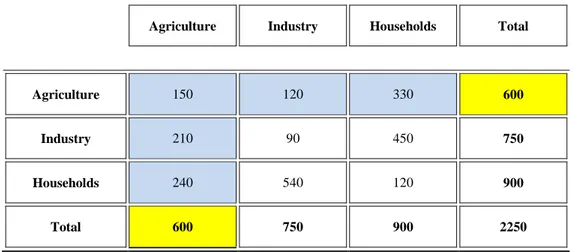
Table 2 - Simplified model for a 3-sector economy (currency units)

Agriculture Industry Households Total

Agriculture 150 120 330 600

Industry 210 90 450 750

Households 240 540 120 900

Total 600 750 900 2250

The mathematics of an input-output matrix is straightforward, but the data requirements are massive since the expenditures and revenues of each branch of the economy have to be represented. Nevertheless the Input-Output methodology is a useful tool for assessing economic impacts of policies and for investigating production relations among primary factors, intersectoral flows, final demands, and transfers.

1. Methodological background

“Economics accounting is based on a fundamental principle of economics: for every income or

receipt there is a corresponding expenditure or outlay. This principle underlies the double-entry accounting procedures that make up the macroeconomic accounts of any country. A SAM is a form of single-entry accounting. SAMs also embody the fundamental principle, but they record transactions between accounts in a square tableau or matrix format(J. F. Francois, 1997).

The Social Accounting Matrix (SAM) is a matrix that compiles all the monetary flows among agents and sectors from a particular economy. It is a systematic method of representing the flows of goods/services and factors and the corresponding payments in an economic system (Stone & Brown, 1962).

With a social accounting matrix we can perform other type of investigations not allowed using the I-O tables (Miller & Blair, 2009).

SAM's were originally developed in Cambridge, UK, by R. Stone (Stone, 1962).The first SAM in 1962 was built as a matrix representation of the National Accounts, and was adopted by the World Bank with Graham Pyatt in the 1960s (Pyatt had worked for Richard Stone at the Cambridge Growth Project). Pyatt left Cambridge and “developed SAMs, mainly at the World Bank”,

(11)

10 becoming together with Erik Thorbecke, the leading proponents and developers of SAMs. "By the

early 1980s, CGE models were heavily ensconced as the approach of the World Bank for development analysis. Social Accounting Matrices (SAMs) were similarly a mainstay of Bank analysis, which had been adopted as a presentational device by the CGE modellers" (Mitra-Kahn,

2008).

SAM is a square matrix of data (number of columns equals number of rows) in the sense that all agents (agents typically include industries, factors of production (e.g. labor and capital), household consumers, the government and the rest-of-the-world region3) are both buyers and sellers. Every economic agent in the economy has both a column account ad a row account. Columns represent buyers (expenditures) and rows represent sellers (receipts).

SAMs were created to identify all monetary flows from sources to recipients, within a disaggregated national account. The SAM is read from column to row, so each entry in the matrix comes from its column heading, going to the row heading. Finally columns and rows are added up, to ensure accounting consistency, and the sum by column equals the sum of each corresponding row.

As shown in the following Table 3, in the SAM each cell represents a flow of funds from a source (column) to a recipient (row). It includes information from most transactions, such as the wages firms pay to households, household’s consumption of goods, and taxes and transfers administrated by the Government.

Table3 - SAM for Open Economy

Activities Commodities Factors Households Government

Savings and Investment Rest of world Total Activities Domestic supply Activity income Commodities Intermediate demand Consumption spending (C) Recurrent spending (G) Investment demand (I) Export earnings (E)

Factors Value-added Total factor

income Households Factors payments to households Social transfers Foreign remittances Total household income Government Sales taxes and import tariffs Direct taxes Foreign grants and loans Government income Savings and Investment Private savings Fiscal surplus Current account balance Total savings Rest of world Import payments (M) Foreign exchange outflow

Total Gross output Total supply Total factor spending Total household spending Government expenditure Total investment spending Foreign exchange inflow

Now let’s look ata simple example to highlight the differences between the I-O and SAM accounts representation framework (Miller & Blair, 2009).

(12)

11

Table4 - I-O and SAM tables from Miller and Blair (2009)

Table 4.

Input – Output representation

Nat. Res. Manuf. Services Households Total Output

Natural Resources 50 30 0 60 140 Manufacturing 60 40 40 40 180 Services 0 0 0 100 100 Value Added Labor 10 70 10 Capital 20 40 50 Total Inputs 140 180 100 Table 5.

SAM Framework Example Using Social Accounting Conventions

Expenditures

Nat. Res. Manuf. Services Labor Capital Households Total Output Income Natural Resources 50 30 0 60 140 Manufacturing 60 40 40 40 180 Services 0 0 0 100 100 Value Added Labor 10 70 10 Capital 20 40 50 Households 90 110 Total Inputs 140 180 100 90 110 200

Source: Miller and Blair 2009.

In the SAM framework, we consider a much more detailed picture of the economy including not only the input–output table of inter-industry income and output, but also the institutional income and expenditures associated with final demand and value added sectors. The SAM framework also provides essentially a complete accounting of the circular flow of income and expenditure in an economy.

SAMs can be easily extended to include other flows in the economy, simply by adding more columns and rows, once the Standard National Account (SNA) flows have been set up. Often rows for ‘capital’ and ‘labour’ are included, and the economy can be disaggregated into any number of sectors. Each extra disaggregated source of funds must have an equal and opposite recipient. So the SAM simplifies the design of the economy being modelled.

SAMs are currently in widespread use, and many statistical bureaus, particularly in OECD countries, create both National Accountsand this matrix counterpart. A theoretical SAM always balances, but empirically estimated SAM’s never do in the first collation. This is due to the problem of converting national accounting data into money flows and the introduction of non-SNA data, compounded by issues of inconsistent national accounting data (which is prevalent for many developing countries, while developed countriestend to include a SAM version of the national account, generally accurateto within 1% of GDP).

This was noted as early as 1984 by Mansur and Whalley, and numerous techniques have been devised to ‘adjust’ SAMs, as “inconsistent data estimated with error, [is] a common experience in many countries”. The traditional method of balancea SAM is based on an iterative process that adjusts each individual cell until the row and column totals became equal.

(13)

12 The RAS method is the most widely known and commonly used automatic procedure for balancing an Input – Output matrix4: this chapter gives a formal description of such a procedure (J. F. Francois, 1997). As expected, there is considerable literature reference on the RAS method, either as part of a more general class of mathematical procedures, both as an economic statistics method (Di Palma, 2005).

The amount of statistical information required for the construction of an input-output table is significant: calculations are complex and laborious, processing time is considerable and so national statistics institutes generally perform this kind of work only every 4-5 years. The methods and evaluation procedures are extremely variable; a series of continuous operations and harmonization are performed from time to time in a patient mosaic work, using all available statistical data. The general methodology can be summarized in the following phases: firstly, it is necessary to evaluate the "marginal totals" of the table, i.e. the sum of rows and columns of the intermediate flowsmatrix: this involves the construction, for each branch, of the goods and services equilibrium account, the production account and the value added distribution account.

This work starts from the evaluation of the supply flows, namely for each sector the production xj

and the imports mj, and then the value added Vj, the total intermediate inputs (xj and mj) and

components of final demand ( Consumption C, Investment I, Export E); then, we proceed to determine the matrix of intermediate flows, which is processed by line, by analyzing by row the sales of intermediate goods and services and by column the cost structure.

The RAS method requires knowledge, for each branch, of the row totals xi. and of the column total

xj. of intermediate outputs and inputs of goods and services: such information can be determined by

knowing the totals of the “frames”, namely the final demand, the intermediate consumptions and the production level. The method also requires the knowledge of a whole matrix at the base year. Generally it is possible to assess directly the majority of the flows of intermediate goods and services, as soon as the necessary data become available. In this case, the application of the RAS method is limited only to the remaining entries.

The method is based on the assumption that the evolution of technical coefficients (see note 5) over time is due to the following factors:

• the price level of the production sector, i.e. the system of relative prices;

• the degree of “absorption” for each good, or the intensity with which a given good has been replaced by (or replaces) other intermediate goods as inputs in the production processes; • the degree of production of each good, i.e. the use of an intermediate input in the production process, as a share of the total of intermediate inputs.

The three above mentioned factors are supposed to operate in uniform way: the first acts of each row and each column, the second on each row and the third on each column of the matrix. To take account of the influence of the above factors it operates in the following way:

First of all the technical coefficients will be corrected to take into account the changes in relative prices. Each technical coefficient of the economic table referredto the year of construction of the matrix (𝑎_𝑖𝑗0_{) will be multiplied by the ratio between changes (from the reference year) of the prices} of the sectors i and j5:

4

It is curious to note that the RAS acronym is generally explained using the name of the economist sir Richard Stone (1919–1991) but this is a matter of debate.

5_{We have:}

(14)

13 1 𝑎_𝑖𝑗∗ = 𝑎_𝑖𝑗0 ∗_𝑝𝑝𝑖

𝑗

Using matrix notation we can write:

2. 𝐴∗= 𝑝̂𝐴0𝑝̂−1

where: 𝐴₀𝑖𝑠 𝑡ℎ𝑒 technical coefficients matrix of the base year 𝐴∗_{𝑖𝑠𝑡technical coefficients matrix} modified from price effect 𝑝̂diagonal matrix of the price index between base year and update year 𝑝̂−1_{inverse matrix of the above diagonal matrix Then we must take into account the system} modification due to changes in the absorption (r) and fabrication (s) degrees of each good6. To perform this, each technical coefficients modified in the previous step, 𝑎_𝑖𝑗∗_{, will be multiplied for (r)} and (s). In matrix notation we can write: 𝐴_𝑡 = 𝑟̂𝐴∗_{𝑠̂where: 𝐴}

𝑡 is the technical coefficients matrix modified from (r) and (s) effects on each good 𝑟̂ is the diagonal matrix that take account of the variations in the sales (r), 𝐴∗_{is the diagonal matrix of the price index between base year and update} year and 𝑠̂ diagonal matrix that take account of the variations in the fabrication processes (r) The updated coefficients can be writing as follow:

3. 𝑎_𝑖𝑗𝑡 = 𝑟𝑖(𝑎𝑖𝑗∗)𝑠𝑗

Substituting 𝑎_𝑖𝑗∗ with(𝑎_𝑖𝑗0 𝑝𝑖

𝑝𝑗) we have: 4.𝑎_𝑖𝑗𝑡 = 𝑟_𝑖(𝑎_𝑖𝑗0 𝑝𝑖

𝑝𝑗) 𝑠𝑗

And, then the new value added coefficients:

1. 𝑣𝑗= [1 − ∑𝑛𝑖=1𝑟𝑖(𝑎𝑖𝑗0 𝑝_𝑝_𝑗𝑖) 𝑠𝑗]

The elements of (r) and (s) matrix are obtained by an iterative procedure based on a set of economic variables at the base year: X gross production, M imports of goods and services, V value added at factors cost, T indirect taxes, C public and private expenditures, I gross investment, E exports of goods and services. On the base of the above dataset, we determine the totals of purchases and sales of intermediate goods, and the marginal distributions of the table:

6. 𝑢𝑖 = [(𝑋𝑖+ 𝑀𝑖) − (𝐶𝑖+ 𝐼𝑖+ 𝐸𝑖)] 7. 𝑧_𝑗 = [𝑋_𝑗− (𝑉_𝑗+ 𝑇_𝑗)]

that demonstrates the above expression.

6

(15)

14 where: 𝑢𝑖 IS sales of goods and services of sector i to other sectors 𝑧𝑗 purchases of goods and services of sector i from other sectors. Calculation of the above vectors starts from the matrix (A*) multiplied by the production vector with respect to the constraint represented by U, until the iterative process, after a certain number of steps, gives (r) and (s). Formally, at year t:

8. 𝐴𝑡∗ 𝑋 = 𝑢 9. 𝑋̂𝐴𝑡′ ∗ 𝐼 = 𝑧

Where the symbols are already defined and I is the identity vector. At matrix is obtained by A

*

as follow:

10. 𝐴∗∗ 𝑋 = 𝑢0

Generally 𝑢₀≠ 𝑢: to get the second term equal to 𝑢 both terms are divided by 𝑢₀ and multiplied times𝑢; so:

11. (𝑢̂𝑢̂₀−1𝐴∗)𝑋 = 𝑢

The product (𝑢̂𝑢̂₀−1_𝐴∗_{) is a further correction of the original matrix 𝐴}

0: we can satisfy the other condition (𝑋̂𝐴_𝑡′ _{∗ 𝐼 = 𝑧) operating:}

12. 𝑋̂(𝐴′∗𝑢̂𝑢̂₀−1)𝐼 = 𝑧₀

Normally 𝑧₀≠ 𝑧 and to get the equality between the two expressions we divide both the terms by 𝑧0 then multiply them times 𝑧. We get:

13. 𝑋̂(𝑧̂𝑧̂0−1𝐴′∗𝑢̂𝑢̂0−1)𝐼 = 𝑧0

At this point, A can be used as correct matrix and the iteration givesa new vector of sales: 14.(𝑢̂𝑢̂₀−1_𝐴∗_𝑧̂𝑧̂ 0−1)𝑋 = 𝑢1 then: 14. (𝑢̂2𝑢̂₀−1𝑢̂₁−1𝐴∗𝑧̂𝑧̂₀−1)𝑋 = 𝑢 repeating 13: 15. 𝑋̂(𝑧̂𝑧̂0−1𝐴′∗𝑢̂2𝑢̂0−1𝑢̂1−1)𝐼 = 𝑧1 To match with the z vector we have:

16. 𝑋̂(𝑧̂2𝑧̂0−1𝑧̂1−1𝐴′∗𝑢̂2𝑢̂0−1𝑢̂1−1)𝐼 = 𝑧

(16)

15 18. (𝑢̂𝑘+1𝑢̂0−1𝑢̂1−1… 𝑢̂𝑘−1𝐴∗𝑧̂0−1𝑧̂1−1… 𝑧̂𝑘−1−1 )𝑋 = 𝑢

19. 𝑋̂(𝑧̂𝑘+1𝑧̂0−1𝑧̂1−1… 𝑧̂𝑘−1𝐴′∗𝑢̂𝑘+1𝑢̂0−1𝑢̂1−1… 𝑢̂𝑘−1)𝐼 = 𝑧

Fixing an appropriate threshold, the iteration process will converge to a finite solution. At the last iteration, the resultingmatrix will be as follows:

20. (𝑢̂𝑘+1𝑢̂₀−1𝑢̂₁−1… 𝑢̂_𝑘−1 )𝐴(∗𝑧̂𝑘+1𝑧̂₀−1𝑧̂₀−1… 𝑧̂_𝑘−1) ≅ 𝐴_𝑡 The r and s vector will be calculated by the following expressions:

21. 𝑟̂ ≅ 𝑢̂𝑘+1𝑢̂₀−1𝑢̂₁−1… 𝑢̂_𝑘−1

22. 𝑠̂ ≅ 𝑧̂𝑘+1𝑧̂0−1𝑧̂1−1… 𝑧̂𝑘−1

The iteration process continues until the totals between rows and columns display an acceptable difference margin, an adequate correspondence threshold error between the two vectors. The research on iterative proportional fitting procedures was firstly related to a probabilistic class of problem in the first half of the last century (Deming & Stephan, 1940), then extended to a several mathematical class of problem and finally demonstrated (Fienberg, 1970) .

(17)

16

1.1 The implemented variant for the case study

Application of a modified version of the standard RAS method is not unusual (Jian, 2002). The used method fall in the so-called category of "biproportion with Known Interior Information methods" (Lahr & De Mesnard, 2004).The proposed variant follows the standard method about the object of the projection, that is the base matrix (applied on the flows and not on the coefficient) without further elaboration (Heng TOH, 1998). The analysis was focused only on historical data of Italy SAM for years 2005 and 2010 and hasn’t involved any type of simulation, like those from bootstrap or Monte Carlo techniques (Jian, 2002) or from the problem of ranking the data quality in estimation (Rodrigues, 1014), since the main focus was to obtain a first order assessment of accuracy gain like a specific type of “constraints configuration”.

The implemented variant for the canonical algorithm used,get the solution in two steps, excluding the cases in which indirect “undesired blocks”to other sectors respect the selected ones (typically when such a sectors contains all zeros but the rows/columns in common with the blocked ones) stop the balancing.

The algorithm doesn’t use a specific treatment of zero in the blocking system or in the rest of the matrix in order to incorporate known information (Paelinck & Waelbroeck, 1982). The logical scheme is based on a sort of two-stage RAS: from this point of view point, the used variant appears similar to TRAS method, (Gilchrist & St. Louis, 1999)

First of all, a RAS method simple variant has been implemented and applied starting from the Italian SAM for the year 2005 to obtain the 2010 Italian SAM. In particular, using these data we have assumed unknown the intersectoral flows, taking as known only the row and column totals and the total value of the production at the projected year.

Next, three distinguished procedure that can be identified as “row-type”, “column-type” and "cross type" has been applied. The procedureinvolves the execution ofthe RAS modified method using different set of constraints, blocking the entire cell on the rows, on the columns and on both the rows and the columns for each sector. Finally, it was performed a balancing process blocking a groups of sectors in the “cross-type configuration”and the results obtained from the different balancing were compared.

It must be noted that the "total lock" for a sector is not possible in all cases (particularly when the block of rows and cells does not coincide with the new estimated value for the total, also if only for the row or the column).

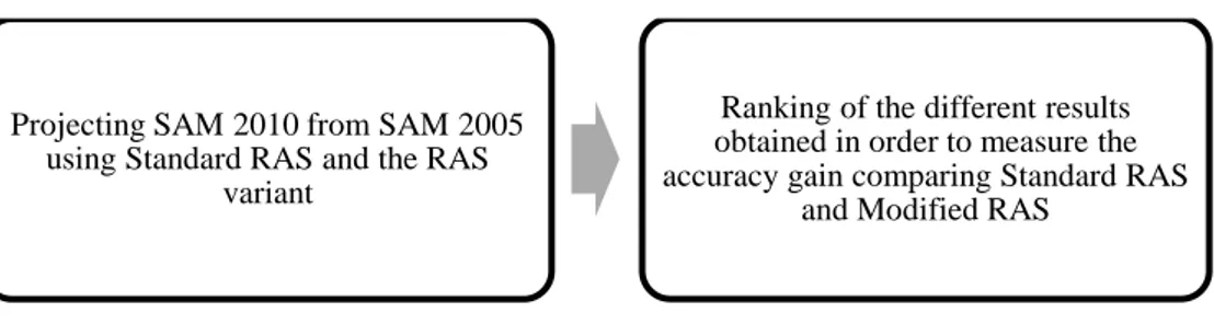
The program was created in an .xlsm file, using a set of routines developed in Visual Basic for Applications7 (see Appendix 2 for the code) under the following logical work-scheme:

7

(18)

17

Figure 1 - Logical work scheme of the analysis

The constraint systemshave beenpracticallyimplementedby means of twodifferent routines:

1.

the first creates and appliesthe constraints to the matrix, by highlighting the blocked cells with a color

2. the second performs the modified RAS(the procedure "reads" the color in each cell and "blocks" the colored cell that contain the constraints)

At the operationallevel, the algorithm, after the canonic first iterative step provided by RAS method, performsthe following operations:

1. the difference between the new total obtained by RAS iteration and the objective total (by row or by column) is calculated;

2. the number of the available free cells and their sum is calculated

3. the share of the difference assigned to each free cell on the basis of the proportion on the free cell sum represented by each cell is now added to the coefficient/flows calculated by RAS

Steps from 1 to 3 involve a simple add to the basic RAS formulas like:

23. 𝑎

_𝑖𝑗

= 𝑎

_{𝑖𝑗𝑅𝐴𝑆}

+ 𝑑𝑖𝑓𝑓 ∗ 𝑠

_𝐹𝑟𝐶

Where:

𝑎_𝑖𝑗 is the estimated final coefficient/flows

𝑎_{𝑖𝑗𝑅𝐴𝑆} is the coefficient/flows estimated by RAS

𝑑𝑖𝑓𝑓 is the difference between the new total by RAS iteration and the objective total (by row or by column)

𝑠_𝐹𝑟𝐶is the share of 𝑎_𝑖𝑗 on total free cell sum

Projecting SAM 2010 from SAM 2005 using Standard RAS and the RAS

variant

Ranking of the different results obtained in order to measure the accuracy gain comparing Standard RAS

(19)

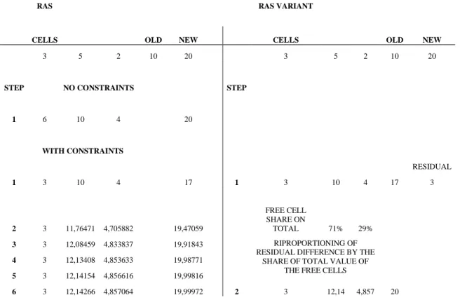
18 To illustrate the speed gain by the use of the modified procedure, consider the following example, relating to the proportional fitting of a line with only three cells:

Figure 2– An intuitive example of the speed gain in iterative proportioning between standard RAS and the used variant

RAS RAS VARIANT

CELLS

OLD NEW CELLS

OLD NEW

3 5 2 10 20 3 5 2 10 20

STEP NO CONSTRAINTS STEP

1 6 10 4 20 WITH CONSTRAINTS RESIDUAL 1 3 10 4 17 1 3 10 4 17 3 2 3 11,76471 4,705882 19,47059 FREE CELL SHARE ON TOTAL 71% 29% 3 3 12,08459 4,833837 19,91843 RIPROPORTIONING OF

RESIDUAL DIFFERENCE BY THE SHARE OF TOTAL VALUE OF

THE FREE CELLS

4 3 12,13408 4,853633 19,98771

5 3 12,14154 4,856616 19,99816

6 3 12,14266 4,857064 19,99972 2 3 12,14 4,857 20

As table 1 shows, without constraints, the standard RAS method fits the row in one step; with the constraints, the variant is balanced in 2 step, while the pure RAS requires at least 5-6 step to obtain an acceptable fit: clearlythe required number of iterations is directly correlated with the selected threshold.

The used threshold in the analysis was fixed at 5 million euros8 (total threshold: 0,00007% of total value of 2010 SAM).

The main criticalities of the variant consists in the fact that, each time the constraints application involves the total block of a row (and a/or a column), there is the possibilites that no solution is available.For example, if, blocking two sectors, another sector hasall the remaining cells (except those related to the blocked sector)set to zero, the balance will be possible only in the case of the new total and the old total results are equal. This is related also to the value of the threshold.

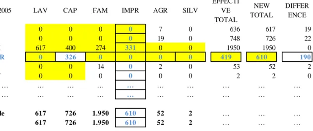
To give a look of the abovementioned situation, see figure below:

8

The threshold was fixed at a rather high level, in order to allow the evaluation of different economic activity sector that otherwise would not be assessable.

(20)

19

Figure 3–An example of infeasibility in balancing adding constraints by row - Projection of Italy SAM 2005 to 2010

Figure 3 shows an excerpt of the matrix related to a case occurred in projecting Italy SAM of year 2005 to year 2010 at the moment of blocking FAMIGLIE sector. Looking at the intersection of CAPITALE and IMPRESE: balancing CAPITALE by column (726 billion) involves the impossibility of row balancing for IMPRESE (the other value on the IMPRESE row are equal to 0; only the sell to GOVERNO sector is available to fitting procedure; but the selected method, based on conservative criteria, unable this cell to compensate the total difference residual, that is in the order of 200 billion of euros). The only value available and useful to balance, cell at the intersection of CAPITALE and IMPRESE (326 billion of euros) do not compensate simultaneously IMPRESE by row and CAPITALE by column.

This kind of problem occur when a cell have to be set to a value that balance by row totally different respect to the one needed to balance by column. This type of situation can be overcome only when the difference is very small (in the order of some million of euros), while in some cases the difference can be assume values around an hundred billions of euros. In this case, the simple practical variant implemented, do not allow the balancing.

Reminding the most basic two definitions of accuracy (partitive and holistic) we recall that the former regard the cell-by-cell accuracy, the latter the second the possibility that the updated matrix represent faithfully the real economic structure. The detail discussion of this problem can be found in (Jensen, 1980) article. In this work, the accuracy is with respectto partitive accuracy, so the considered error is equal to the distance between target matrix and estimated matrix.

Finally, in order to quantify the deviations of results between methods, among several indicators we have chosen MAE (Mean Absolute Error), MAPE (Mean Absolute Percentage Error), STPE (Standardized Total Percentage Error) and RMSE (Root Mean Square Error)9; STPE is the preferred measure indicator of error because of its stability.

The formulas of the chosen indicators are:

24. 𝑀𝐴𝐸 = ∑𝑛𝑖=1∑𝑛𝑗=1|𝑎𝑖𝑗𝑡 − 𝑎𝑖𝑗𝑓|/𝑛 9

See (Swanson, Tayman, & Bryan, 2011).

2005 LAV CAP FAM IMPR AGR SILV

EFFECTI VE TOTAL NEW TOTAL DIFFER ENCE LAV 0 0 0 0 7 0 636 617 19 CAP 0 0 0 0 19 0 748 726 22 FAM 617 400 274 331 0 0 1950 1950 0 IMPR 0 326 0 0 0 0 419 610 190 AGR 0 0 14 0 2 0 53 52 2 SILV 0 0 0 0 0 0 2 2 0 … … … … … … … … … … … … … … … … … … … … Totale 617 726 1.950 610 52 2 … … … 617 726 1.950 610 52 2 … … …

(21)

20 25. 𝑀𝐴𝑃𝐸 = ∑ ∑ |𝑎𝑖𝑗 𝑡_−𝑎 𝑖𝑗 𝑓 𝑎_𝑖𝑗𝑓 | /𝑛 𝑛 𝑗=1 𝑛 𝑖=1 26. 𝑆𝑇𝑃𝐸 = ∑𝑛_𝑖=1∑_𝑗=1𝑛 |𝑎_𝑖𝑗𝑓 − 𝑎_𝑖𝑗𝑡|/ ∑𝑛_𝑖=1∑𝑛_𝑗=1𝑎_𝑖𝑗1 27. 𝑅𝑀𝑆𝐸 = √1 𝑛∑ (𝑎𝑖𝑗 𝑡 _{− 𝑎} 𝑖𝑗𝑓) 2 𝑛 𝑖=1

Where 𝑛represent the total number of cells and |𝑎𝑖𝑗𝑡 − 𝑎𝑖𝑗𝑓| represents the elements of the target matrix and of forecast matrix, respectively.

(22)

21

2. Results

The main indicators selected to measure accuracy in projecting SAM give the following result for Standard RAS:

MAE=1266,532; MAPE= 15,200; RMSE= 15042,678; STPE=0,601

The following tables reports the data obtained from balancing processes by blocking each sector one by one in, respectively, row, column and “cross” configurations.

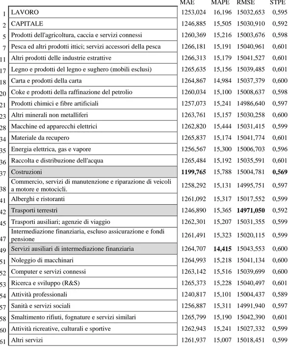
Table 5- Base results - rows blocked one by one

Row-Type Configuration

MAE MAPE RMSE STPE

1 LAVORO 1253,024 16,196 15032,653 0,595

2 CAPITALE 1246,885 15,505 15030,910 0,592

5 Prodotti dell'agricoltura, caccia e servizi connessi 1260,369 15,216 15003,676 0,598 7 Pesca ed altri prodotti ittici; servizi accessori della pesca 1266,181 15,191 15040,961 0,601 11 Altri prodotti delle industrie estrattive 1266,313 15,179 15041,527 0,601 17 Legno e prodotti del legno e sughero (mobili esclusi) 1265,635 15,156 15039,485 0,601

18 Carta e prodotti della carta 1264,867 14,984 15037,379 0,600

20 Coke e prodotti della raffinazione del petrolio 1260,034 15,100 15008,637 0,598 21 Prodotti chimici e fibre artificiali 1257,073 15,241 14986,640 0,597 23 Altri minerali non metalliferi 1263,761 15,157 15030,258 0,600 28 Macchine ed apparecchi elettrici 1262,820 15,444 15031,415 0,599

34 Materiale da recupero 1265,837 15,174 15041,774 0,601

35 Energia elettrica, gas e vapore 1256,567 15,300 15006,703 0,596 36 Raccolta e distribuzione dell'acqua 1265,484 15,192 15035,591 0,601

37 Costruzioni 1199,765 15,788 15004,781 0,569

38

Commercio, servizi di manutenzione e riparazione di veicoli

a motore e motocicli. 1258,292 15,131 14995,751 0,597

41 Alberghi e ristoranti 1261,092 15,317 15017,552 0,599

42 Trasporti terrestri 1246,890 15,365 14971,050 0,592

45 Trasporti ausiliari; agenzie di viaggio 1262,301 15,207 15031,355 0,599 47

Intermediazione finanziaria, escluso assicurazione e fondi

pensione 1261,491 15,323 15020,115 0,599

49 Servizi ausiliari di intermediazione finanziaria 1264,707 14,415 15043,553 0,600

51 Noleggio di macchinari 1264,993 15,218 15041,134 0,600

52 Computer e servizi connessi 1263,142 15,516 15039,699 0,600

53 Ricerca e sviluppo (R&S) 1265,373 15,228 15040,497 0,601

54 Attività professionali 1240,817 15,101 15004,437 0,589

57 Sanità e servizi sociali 1256,887 15,311 14991,940 0,597

58 Smaltimento rifiuti, fognature e servizi similari 1265,799 15,190 15042,390 0,601 60 Attività ricreative, culturali e sportive 1262,943 15,241 15027,332 0,599

(23)

22

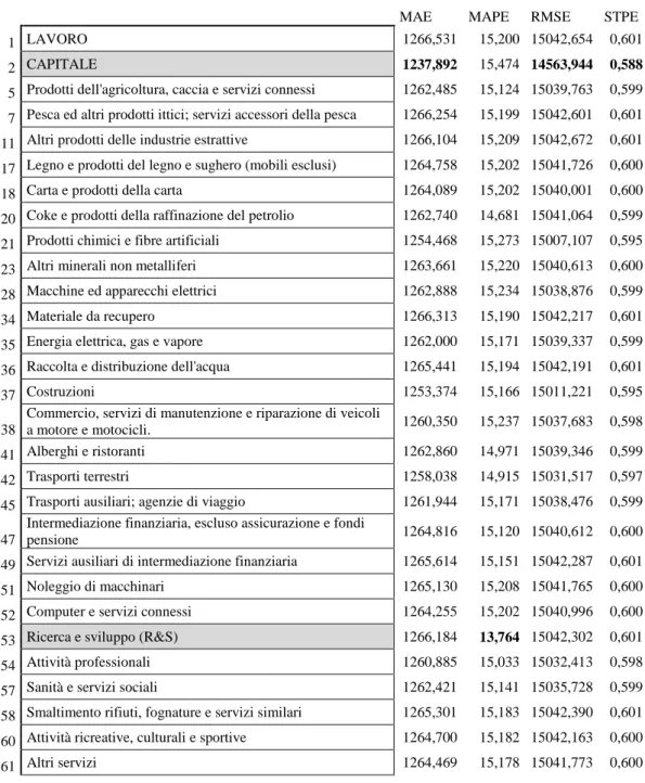
Table 6- Base results - columns blocked one by one

Column-Type Configuration

MAE MAPE RMSE STPE

1 LAVORO 1266,531 15,200 15042,654 0,601

2 CAPITALE 1237,892 15,474 14563,944 0,588

20 Coke e prodotti della raffinazione del petrolio 1262,740 14,681 15041,064 0,599 21 Prodotti chimici e fibre artificiali 1254,468 15,273 15007,107 0,595

23 Altri minerali non metalliferi 1263,661 15,220 15040,613 0,600

28 Macchine ed apparecchi elettrici 1262,888 15,234 15038,876 0,599

37 Costruzioni 1253,374 15,166 15011,221 0,595

38

42 Trasporti terrestri 1258,038 14,915 15031,517 0,597

pensione 1264,816 15,120 15040,612 0,600

49 Servizi ausiliari di intermediazione finanziaria 1265,614 15,151 15042,287 0,601

53 Ricerca e sviluppo (R&S) 1266,184 13,764 15042,302 0,601

61 Altri servizi 1264,469 15,178 15041,773 0,600

Respect to the table 1, blocking columns involves that the minimum errors move from the "middle internal area” of the SAM to the “high” part of the matrix. In particular, the “CAPITALE” sector, reports the best values for MAE, STPE and RMSE. The relationships between accuracy improvement provided by each sector and its specific position in the matrix area will be investigate in the follows, when we’ll correlatethe multipliers value10of the blocked sectors and their contribution to decreasing of error indicators.

10

The exam of the SAM multipliers matrix, both for year 2005 and year 2010, shows a concentration of the multipliers value on the diagonal and on the institutional sectors (see Appendix 1 - Multipliers).

(24)

23

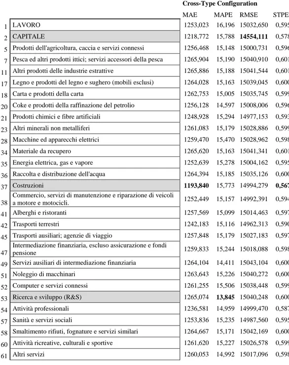
Table 7- Base results - rows and columns simultaneously blocked one by one for each sector

Cross-Type Configuration

MAE MAPE RMSE STPE

1 LAVORO 1253,023 16,196 15032,650 0,595

2 CAPITALE 1218,772 15,788 14554,111 0,578

20 Coke e prodotti della raffinazione del petrolio 1256,128 14,597 15008,006 0,596 21 Prodotti chimici e fibre artificiali 1248,928 15,294 14977,153 0,593 23 Altri minerali non metalliferi 1261,083 15,179 15028,886 0,599 28 Macchine ed apparecchi elettrici 1259,470 15,470 15028,962 0,598

37 Costruzioni 1193,840 15,773 14994,279 0,567

38

42 Trasporti terrestri 1242,183 15,116 14962,313 0,590

pensione 1259,833 15,244 15018,088 0,598

49 Servizi ausiliari di intermediazione finanziaria 1264,104 14,411 15043,104 0,600

53 Ricerca e sviluppo (R&S) 1265,074 13,845 15040,248 0,600

61 Altri servizi 1260,053 14,992 15017,096 0,598

The distribution of the errors in matrix areas is analyzed in detail in the Appendix 1 – Distribution

of the errors and suggests a prevalence of the “High” and “Middle” areas respect to the “Low” area

about the effects of the constraints application in terms of decreasing of the errors measured by MAE, MAPE, RMSE and STPE.

It’s now interesting compare the multipliers values to the error performance for each sector in the different type of constraints configuration. Before of this, its useful report the performance of each sector in terms of change of the selected indicators, in all the three constraints configuration schemes, respect to the Standard RAS method.

(25)

24 Fi g u re 4 –Co n tr ib u tio n o f e a c h b lo c k e d se cto r to p e rc e n ta g e d e cr ea sin g o f se le cte d i n d ica to rs - % R o w -Ty p e C o lu m n -Ty p e C ro s s -Ty p e M A E M A P E R M S E S TP E M A E M A P E R M S E S TP E M A E M A P E R M S E S TP E 1 -1 ,0 7 % 6 ,5 5 % -0 ,0 7 % -1 ,0 7 % 0 ,0 0 % 0 ,0 0 % 0 ,0 0 % 0 ,0 0 % -1 ,0 7 % 6 ,5 5 % -0 ,0 7 % -1 ,0 7 % 2 -1 ,5 5 % 2 ,0 1 % -0 ,0 8 % -1 ,5 5 % -2 ,2 6 % 1 ,8 0 % -3 ,1 8 % -2 ,2 6 % -3 ,7 7 % 3 ,8 7 % -3 ,2 5 % -3 ,7 7 % 5 -0 ,4 9 % 0 ,1 1 % -0 ,2 6 % -0 ,4 9 % -0 ,3 2 % -0 ,5 0 % -0 ,0 2 % -0 ,3 2 % -0 ,7 9 % -0 ,3 5 % -0 ,2 8 % -0 ,7 9 % 7 -0 ,0 3 % -0 ,0 6 % -0 ,0 1 % -0 ,0 3 % -0 ,0 2 % -0 ,0 1 % 0 ,0 0 % -0 ,0 2 % -0 ,0 5 % -0 ,0 7 % -0 ,0 1 % -0 ,0 5 % 11 -0 ,0 2 % -0 ,1 4 % -0 ,0 1 % -0 ,0 2 % -0 ,0 3 % 0 ,0 6 % 0 ,0 0 % -0 ,0 3 % -0 ,0 5 % -0 ,0 8 % -0 ,0 1 % -0 ,0 5 % 17 -0 ,0 7 % -0 ,2 9 % -0 ,0 2 % -0 ,0 7 % -0 ,1 4 % 0 ,0 1 % -0 ,0 1 % -0 ,1 4 % -0 ,2 0 % -0 ,2 4 % -0 ,0 2 % -0 ,2 0 % 18 -0 ,1 3 % -1 ,4 2 % -0 ,0 4 % -0 ,1 3 % -0 ,1 9 % 0 ,0 1 % -0 ,0 2 % -0 ,1 9 % -0 ,3 0 % -1 ,2 9 % -0 ,0 5 % -0 ,3 0 % 20 -0 ,5 1 % -0 ,6 6 % -0 ,2 3 % -0 ,5 1 % -0 ,3 0 % -3 ,4 2 % -0 ,0 1 % -0 ,3 0 % -0 ,8 2 % -3 ,9 7 % -0 ,2 3 % -0 ,8 2 % 21 -0 ,7 5 % 0 ,2 7 % -0 ,3 7 % -0 ,7 5 % -0 ,9 5 % 0 ,4 8 % -0 ,2 4 % -0 ,9 5 % -1 ,3 9 % 0 ,6 1 % -0 ,4 4 % -1 ,3 9 % 23 -0 ,2 2 % -0 ,2 8 % -0 ,0 8 % -0 ,2 2 % -0 ,2 3 % 0 ,1 3 % -0 ,0 1 % -0 ,2 3 % -0 ,4 3 % -0 ,1 4 % -0 ,0 9 % -0 ,4 3 % 28 -0 ,2 9 % 1 ,6 0 % -0 ,0 7 % -0 ,2 9 % -0 ,2 9 % 0 ,2 2 % -0 ,0 3 % -0 ,2 9 % -0 ,5 6 % 1 ,7 7 % -0 ,0 9 % -0 ,5 6 % 34 -0 ,0 5 % -0 ,1 8 % -0 ,0 1 % -0 ,0 5 % -0 ,0 2 % -0 ,0 7 % 0 ,0 0 % -0 ,0 2 % -0 ,0 7 % -0 ,2 5 % -0 ,0 1 % -0 ,0 7 % 35 -0 ,7 9 % 0 ,6 6 % -0 ,2 4 % -0 ,7 9 % -0 ,3 6 % -0 ,1 9 % -0 ,0 2 % -0 ,3 6 % -1 ,1 0 % 0 ,5 1 % -0 ,2 6 % -1 ,1 0 % 36 -0 ,0 8 % -0 ,0 6 % -0 ,0 5 % -0 ,0 8 % -0 ,0 9 % -0 ,0 4 % 0 ,0 0 % -0 ,0 9 % -0 ,1 7 % -0 ,1 0 % -0 ,0 5 % -0 ,1 7 % 37 -5 ,2 7 % 3 ,8 7 % -0 ,2 5 % -5 ,2 7 % -1 ,0 4 % -0 ,2 3 % -0 ,2 1 % -1 ,0 4 % -5 ,7 4 % 3 ,7 7 % -0 ,3 2 % -5 ,7 4 % 38 -0 ,6 5 % -0 ,4 6 % -0 ,3 1 % -0 ,6 5 % -0 ,4 9 % 0 ,2 4 % -0 ,0 3 % -0 ,4 9 % -1 ,1 1 % -0 ,2 8 % -0 ,3 3 % -1 ,1 1 % 41 -0 ,4 3 % 0 ,7 7 % -0 ,1 7 % -0 ,4 3 % -0 ,2 9 % -1 ,5 1 % -0 ,0 2 % -0 ,2 9 % -0 ,7 1 % -0 ,6 7 % -0 ,1 9 % -0 ,7 1 % 42 -1 ,5 5 % 1 ,0 8 % -0 ,4 8 % -1 ,5 5 % -0 ,6 7 % -1 ,8 8 % -0 ,0 7 % -0 ,6 7 % -1 ,9 2 % -0 ,5 5 % -0 ,5 3 % -1 ,9 2 % 45 -0 ,3 3 % 0 ,0 5 % -0 ,0 8 % -0 ,3 3 % -0 ,3 6 % -0 ,1 9 % -0 ,0 3 % -0 ,3 6 % -0 ,6 9 % -0 ,1 4 % -0 ,1 0 % -0 ,6 9 % 47 -0 ,4 0 % 0 ,8 1 % -0 ,1 5 % -0 ,4 0 % -0 ,1 4 % -0 ,5 3 % -0 ,0 1 % -0 ,1 4 % -0 ,5 3 % 0 ,2 9 % -0 ,1 6 % -0 ,5 3 % 49 -0 ,1 4 % -5 ,1 7 % 0 ,0 1 % -0 ,1 4 % -0 ,0 7 % -0 ,3 2 % 0 ,0 0 % -0 ,0 7 % -0 ,1 9 % -5 ,1 9 % 0 ,0 0 % -0 ,1 9 % 51 -0 ,1 2 % 0 ,1 2 % -0 ,0 1 % -0 ,1 2 % -0 ,1 1 % 0 ,0 5 % -0 ,0 1 % -0 ,1 1 % -0 ,2 3 % 0 ,1 7 % -0 ,0 2 % -0 ,2 3 % 52 -0 ,2 7 % 2 ,0 8 % -0 ,0 2 % -0 ,2 7 % -0 ,1 8 % 0 ,0 1 % -0 ,0 1 % -0 ,1 8 % -0 ,4 2 % 2 ,0 1 % -0 ,0 3 % -0 ,4 2 % 53 -0 ,0 9 % 0 ,1 8 % -0 ,0 1 % -0 ,0 9 % -0 ,0 3 % -9 ,4 5 % 0 ,0 0 % -0 ,0 3 % -0 ,1 2 % -8 ,9 2 % -0 ,0 2 % -0 ,1 2 % 54 -2 ,0 3 % -0 ,6 6 % -0 ,2 5 % -2 ,0 3 % -0 ,4 5 % -1 ,1 0 % -0 ,0 7 % -0 ,4 5 % -2 ,3 6 % -1 ,5 9 % -0 ,2 9 % -2 ,3 6 % 57 -0 ,7 6 % 0 ,7 3 % -0 ,3 4 % -0 ,7 6 % -0 ,3 2 % -0 ,3 9 % -0 ,0 5 % -0 ,3 2 % -1 ,0 0 % 0 ,2 3 % -0 ,3 7 % -1 ,0 0 % 58 -0 ,0 6 % -0 ,0 7 % 0 ,0 0 % -0 ,0 6 % -0 ,1 0 % -0 ,1 1 % 0 ,0 0 % -0 ,1 0 % -0 ,1 5 % -0 ,2 0 % 0 ,0 0 % -0 ,1 5 % 60 -0 ,2 8 % 0 ,2 7 % -0 ,1 0 % -0 ,2 8 % -0 ,1 4 % -0 ,1 2 % 0 ,0 0 % -0 ,1 4 % -0 ,3 9 % 0 ,1 7 % -0 ,1 1 % -0 ,3 9 % 61 -0 ,3 6 % -1 ,2 7 % -0 ,1 6 % -0 ,3 6 % -0 ,1 6 % -0 ,1 5 % -0 ,0 1 % -0 ,1 6 % -0 ,5 1 % -1 ,3 7 % -0 ,1 7 % -0 ,5 1 % S u m -1 8 ,8 0 % 1 0 ,4 2 % -3 ,8 6 % -1 8 ,8 0 % -9 ,7 5 % -1 7 ,2 0 % -4 ,0 7 % -9 ,7 5 % -2 6 ,8 3 % -5 ,4 3 % -7 ,4 8 % -2 6 ,8 3 % M e a n -0 ,6 5 % 0 ,3 6 % -0 ,1 3 % -0 ,6 5 % -0 ,3 4 % -0 ,5 9 % -0 ,1 4 % -0 ,3 4 % -0 ,9 3 % -0 ,1 9 % -0 ,2 6 % -0 ,9 3 %

(26)

25

Where the numbers of sectors follow the below scheme:

1 LAVORO 2 CAPITALE

5 Prodotti dell'agricoltura, caccia e servizi connessi 7 Pesca ed altri prodotti ittici; servizi accessori della pesca 11 Altri prodotti delle industrie estrattive

17 Legno e prodotti del legno e sughero (mobili esclusi) 18 Carta e prodotti della carta

20 Coke e prodotti della raffinazione del petrolio 21 Prodotti chimici e fibre artificiali

23 Altri minerali non metalliferi 28 Macchine ed apparecchi elettrici 34 Materiale da recupero

35 Energia elettrica, gas e vapore 36 Raccolta e distribuzione dell'acqua 37 Costruzioni

38 Commercio, servizi di manutenzione e riparazione di veicoli a motore e motocicli. 41 Alberghi e ristoranti

42 Trasporti terrestri

45 Trasporti ausiliari; agenzie di viaggio

47 Intermediazione finanziaria, escluso assicurazione e fondi pensione 49 Servizi ausiliari di intermediazione finanziaria

51 Noleggio di macchinari 52 Computer e servizi connessi 53 Ricerca e sviluppo (R&S) 54 Attività professionali 57 Sanità e servizi sociali

58 Smaltimento rifiuti, fognature e servizi similari 60 Attività ricreative, culturali e sportive

61 Altri servizi

Figure X shows clearly that blocking a sector in balancing process adds accuracy in projecting SAM. In particular, you can see that for the sectors considered one by one, the average gain in forecasting precision is around the 1% for MAE and STPE, with considerable variations between sectors: see, for MAE in row-type configuration,sector 7 (0.07%) compared to sector 37(-5.27 %).

The complete comparison of the twelve measures of performance of the figure X to the six aggregations of the multipliers (row, column, row-column for the years, 2005 and 2010) is reported in the Appendix 1 – Comparison among multipliers and contribution to error decrease. The comparison is performed, for year 2005 and 2010, correlating each scheme with the decrease of MAE, MAPE, RMSE and STPE coming from corresponding constraints configuration (so, the sum of the multipliers values by row is correlated with the decrease of indicators coming from row constraints scheme).

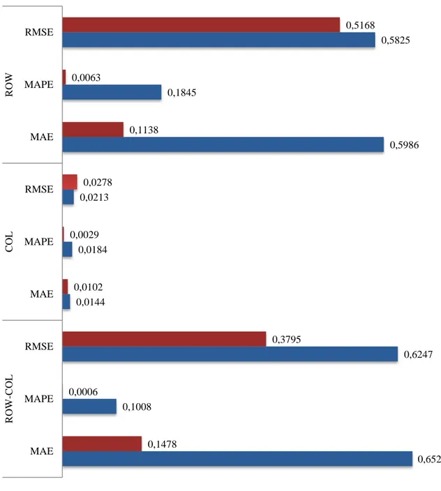
The figure X shows the comparison among the determination coefficient (R2) calculated in the test session reported in the Appendix 1 at the abovementioned section.

The Pearson test indicates that the row-column multipliers sum correlated with the decrease of error indicators coming from row-column configuration constraints show the strong correlation.

(27)

26

Figure 5–R2_{calculated correlating multipliers values for row, column, row-column with the decrease of MAE}11_,

MAPE, RMSE from balancing, for the three constraints configurations

Naturally, the results reported in the above figure are not sufficient to postulate functional relationships between multipliers values and capacity of related sectors, if blocked in RAS balancing, to resolve in accuracy gain when projecting matrix. However, the test performed, seems to indicate an interest about further investigation about this point.

11

The STPE results, in terms of percentage decrease of error to Standard RAS, are equal to MAE and, therefore, omitted. 0,6520 0,1008 0,6247 0,0144 0,0184 0,0213 0,5986 0,1845 0,5825 0,1478 0,0006 0,3795 0,0102 0,0029 0,0278 0,1138 0,0063 0,5168 MAE MAPE RMSE MAE MAPE RMSE MAE MAPE RMSE R O W-C O L C OL R OW 2010 2005

(28)

27

Combined constraints

It seems reasonable, on the basis of what previously established, investigate on the effects produced when the sectors are simultaneously blocked in a cumulative balancing iteration. The test was performed only for MAE, to get a first order assessment of the effects.

Table 8- Accuracy gain in forecasting SAM 2010 by blocking a cumulative set of sectors

MAE decrease Sum of single contribution to MAE decrease

2+37 -9,27% -9,51% 2+37+54 -11,12% -11,88% 2+37+42+54 -12,92% -13,80% 2+21+37+42+54 -14,26% -15,19% 2+21+37+38+42+54 -15,26% -16,30% 2+21+35+37+38+42+54 -16,24% -17,40% 2+21+35+37+38+42+54+57 -17,29% -18,12% 2+20+21+35+37+38+42+54+57 -17,81% -19,22% 2+6+20+21+35+37+38+42+54+57 -18,54% -20,02% 2+6+20+21+35+37+38+42+45+54+57 -19,20% -20,72%

The above table, shows what happens when we block, one by one, the sectors, adding every new sector to the initial ones. So, adding the sector 54 to the 2+37 produces a further decrease of MAE by 1,85% and so on.

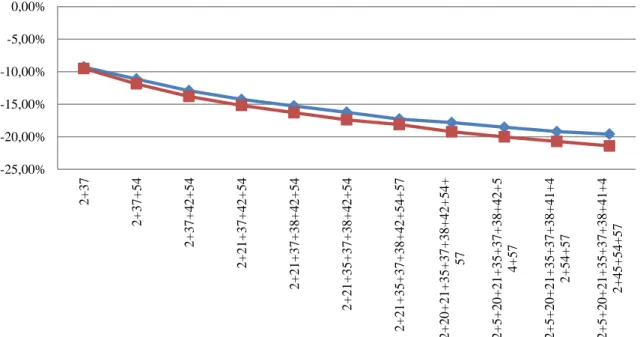
Figure 6 - MAE decreasing from combined cross constraints application compared to sum of single MAE decreasing from blocking each sector one by one

-25,00% -20,00% -15,00% -10,00% -5,00% 0,00% 2 + 3 7 2 + 3 7 + 5 4 2 + 3 7 + 4 2 + 5 4 2 + 2 1 + 3 7 + 4 2 + 5 4 2 + 2 1 + 3 7 + 3 8 + 4 2 + 5 4 2 + 2 1 + 3 5 + 3 7 + 3 8 + 4 2 + 5 4 2 + 2 1 + 3 5 + 3 7 + 3 8 + 4 2 + 5 4 + 5 7 2 + 2 0 + 2 1 + 3 5 + 3 7 + 3 8 + 4 2 + 5 4 + 57 2 + 5 + 2 0 + 2 1 + 3 5 + 3 7 + 3 8 + 4 2 + 5 4 + 5 7 2 + 5 + 2 0 + 2 1 + 3 5 + 3 7 + 3 8 + 4 1 + 4 2 + 5 4 + 5 7 2 + 5 + 2 0 + 2 1 + 3 5 + 3 7 + 3 8 + 4 1 + 4 2 + 4 5 + 5 4 + 5 7

(29)

28 Figure 6 shows the explicative capacity of combined constraints application with respect to single contribute of each sector expressed as the difference between respective trends. So, it can be noted that introducing a new sector (57) modified the decreasing trends (that suggest a greater effect of the combined constraints to the sum of single contribute), probably due to the multipliers effects in the balancing process12.

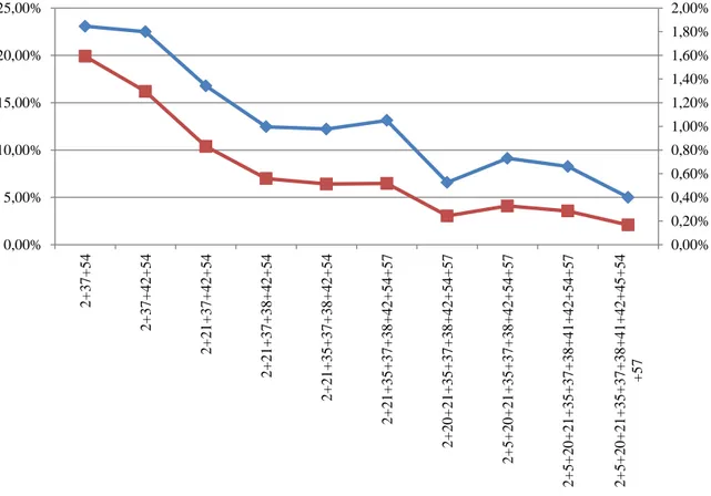
Figure 7 - Percentage difference between MAE estimated by RAS blocking several sector simultaneously

Figure 7 shows the cumulated decrease of MAE when new sectors are blocked together with the initial one. So, moving from sector 2+37+54 (blocked) to 2+37+42+54, we get a decrease of MAE of 1,80 % in absolute terms where the relative measure decreases by of 3,73% (this means that the ratio between the relateddecrease of MAE moves from 19,91% to 16,18%).

12

This type of effects indicate the possibilities of investigate on the relationships between disaggregation grade for matrix and intensity of the effects by application of the constraints, especially in the case of disaggregation focused to specific sector analysis (RAO, CIORBA, TROVATO, NOTARO, & FERRARESE, 2014).

0,00% 0,20% 0,40% 0,60% 0,80% 1,00% 1,20% 1,40% 1,60% 1,80% 2,00% 0,00% 5,00% 10,00% 15,00% 20,00% 25,00% 2 + 3 7 + 5 4 2 + 3 7 + 4 2 + 5 4 2 + 2 1 + 3 7 + 4 2 + 5 4 2 + 2 1 + 3 7 + 3 8 + 4 2 + 5 4 2 + 2 1 + 3 5 + 3 7 + 3 8 + 4 2 + 5 4 2 + 2 1 + 3 5 + 3 7 + 3 8 + 4 2 + 5 4 + 5 7 2 + 2 0 + 2 1 + 3 5 + 3 7 + 3 8 + 4 2 + 5 4 + 5 7 2 + 5 + 2 0 + 2 1 + 3 5 + 3 7 + 3 8 + 4 2 + 5 4 + 5 7 2 + 5 + 2 0 + 2 1 + 3 5 + 3 7 + 3 8 + 4 1 + 4 2 + 5 4 + 5 7 2 + 5 + 2 0 + 2 1 + 3 5 + 3 7 + 3 8 + 4 1 + 4 2 + 4 5 + 5 4 + 5 7

(30)

29

Conclusion

Searching for a better estimate of a matrix based on the structure of a previous oneand margins of another matrix is a very general problem that contain elements of interest for many applications in several research areas (Norman, 1999), (Lahr & De Mesnard, 2004).

Bi-proportional methods are efficient where information is missing, unavailable, and when econometric estimation is at least difficult if not impossible—typically where phenomena are represented by matrices.

The iterative methods proposed in this work can be applied in many fields outside the developing application to National Accounting.

This report presents a variant application, a simple algorithm developed in VBA that measure the accuracy gain in projecting a SAM through the application of different configurations of "cross-type" constraints.

The results suggest that investigatingthe information gain from constraints use is a usefulanalysis that could be improved by comparing the "cross-type" constraints, with different typology set (radial, angular, concentrated in specific areas of the matrix).

(31)

(32)

31

Bibliography

Di Palma, M. (2005). Tecniche di aggiornamento di una tavola delle interdipendenze settoriali. Roma: Università degli Studi di Roma "La Sapienza".

Gilchrist, D. A., & St Louis, L. V. (1999). Completing Input-Output Tables using Partial Information, with an Application to Canadian Data. Economic Systems Research, 185-194,. Gilchrist, D., & St. Louis, L. (1999). Completing input–output tables using partial information with

an application to Canadian data. Economic System Research, 185-193.

Heng TOH, M. (1998). Projecting the Leontief inverse directly by the RAS method. 12th

International Conference on Input-Output Techniques. New York: National University of

Singapore.

Istat. (2009). Classificazione delle Attività Economiche ATECO 2007 derivata dalla NACE rev.

2.Roma: Istat.

J. F. Francois, K. A. (1997). Chapter 4. In K. A. J. F. Francois, Applied Methods for Trade Policy

Analysis: A Handbook (pp. 94-121). 1997: Cambridge University Press.

Jensen, R. C. (1980). The Concept of Accuracy in Regional Input-Output Models. International

Regional Science Review, 139-154.

Jian, X. (2002). Distance, Degree of Freedom and Error of RAS method. Fourteenth International

Conference on Input-Output Techniques . Montreal: Chinese Academy of Science.

Lahr, M., & De Mesnard, L. (2004). Biproportional techniques in input-output analysis: table updating and structural analysis. Economic Systems Research , 115-134.

Leontief, W. (1936). Quantitative Input-Output Relations in the Economic System of the United States. Review of Economic and Statistics, 105-125.

Mesnard, L. d. (2002). Failure of the normalization of the RAS method : absorption and fabrication effects are still incorrect. The Annals of Regional Science, 139-144 .

Miller, R., & Blair, P. (2009). Appendix C Historical Notes on the Development of Leontief’s Input–Output Analysis. In R. Miller, & P. Blair, Input-Output Analysis - Foundations and

Extensions - Second Edition (pp. 724-737). Cambridge: Cambridge University Press.

Mitra-Kahn, B. (2008). Debunking the Myths of Computable General Equilibrium Models. SCEPA Working Paper.

Norman, P. (1999). Putting Iterative Proportional Fitting on the Researcher's Desk. Leeds: University of Leeds.

Paelinck, J., & Waelbroeck, J. (1982). Etude empirique sur l’evolution de coefficients ‘input– output’: essai d’application de la procedure RAS de Cambridge au tableau industriel belge.

Economie Appliquee, 81-111.

Rao, M., & Tommasino, M. C. (2014). Updating technical coefficients of an input-output matrix

with RAS– the TRIOBal software.Roma: ENEA.

Rao, M., Ciorba, U., Trovato, G., Notaro, C., & Ferrarese, C. (2014). Costruzione di una Matrice di

Contabilità Sociale allargata al settore energetico (Energy-Sam) .Roma: Enea.

Rodrigues, J. F. (1014). A Bayesian Approach to the Balancing of Statistical Economic Data.

Entropy, 1243-1271.

Stone, R. &. (1962). A computable model for economic growth. Cambridge Growth Project. Cambridge, U.K.

Swanson, D. A., Tayman, J., & Bryan, T. (2011). MAPE-R: a rescaled measure od accuracy for cross-sectional subnational population forecasts. J Pop Research, 225-243.

(33)

32 Szyrmer, J. (1989). Trade-Off between Error and Information in the RAS Procedure. In R. Miller, K. Polenske, & A. Rose, Frontiers of Input-Output Analysis (pp. 258-277). New York: Oxford University Press.

U.N. (n.d.). Retrieved February 2, 2014, from System of National Accounts 2008: http://synagonism.net/standard/economy/un.sna.2008.html

(34)

33

Appendix 1 - The Social Accounting Matrix for Italy for years 2005 and

2010

General notes

The flows, expressed in currency, reported in the tablesfor years 2005 and 2010represents the following economic activity sectors:

According to the before mentioned classification, the 1 to 4 and 63 to 65 sectors correspond to institutional sectors, the remaining to productive sectors.

1 LAVORO

2 CAPITALE

3 FAMIGLIE

4 IMPRESE

5 Prodotti dell'agricoltura, caccia e servizi connessi 6 Prodotti della silvicoltura e servizi connessi

7 Pesca ed altri prodotti ittici; servizi accessori della pesca

8 Carbon fossile

9 Petrolio e gas naturale; servizi accessori all'estrazione di olio e gas 10 Estrazione di minerali metalliferi

11 Altri prodotti delle industrie estrattive 12 Prodotti alimentari e bevande 13 Industria del tabacco 14 Prodotti tessili 15 Vestiario e pellicce 16 Cuoio e prodotti in pelle

17 Legno e prodotti del legno e sughero (mobili esclusi) 18 Carta e prodotti della carta

19 Editoria e stampa

20 Coke e prodotti della raffinazione del petrolio 21 Prodotti chimici e fibre artificiali

22 Gomma e prodotti in plastica 23 Altri minerali non metalliferi 24 Metalli e leghe

25 Prodotti metallici, eccetto macchine ed apparecchi 26 Macchine ed apparecchi meccanici

27 Macchine per ufficio e computer 28 Macchine ed apparecchi elettrici 29 Apparecchi radiotelevisivi

30 Apparecchi medicali, di precisione, strumenti ottici ed orologi 31 Veicoli a motore e rimorchi

32 Altri mezzi di trasporto

33 Mobili ed altri prodotti manifatturieri 34 Materiale da recupero

(35)

34

36 Raccolta e distribuzione dell'acqua

37 Costruzioni

38 Commercio, servizi di manutenzione e riparazione di veicoli a motore e motocicli.

39 Commercio all'ingrosso, esclusi veicoli a motore e motocicli 40 Commercio al dettaglio, esclusi veicoli a motore e motocicli 41 Alberghi e ristoranti

42 Trasporti terrestri 43 Trasporti marittimi 44 Trasporti aerei

45 Trasporti ausiliari; agenzie di viaggio 46 Poste e telecomunicazioni

47 Intermediazione finanziaria, escluso assicurazione e fondi pensione 48 Assicurazione e fondi pensione, esclusa previdenza sociale obbligatoria 49 Servizi ausiliari di intermediazione finanziaria

50 Attività immobiliari 51 Noleggio di macchinari 52 Computer e servizi connessi 53 Ricerca e sviluppo (R&S) 54 Attività professionali

55 Pubblica amministrazione e difesa; previdenza sociale obbligatoria

56 Istruzione

57 Sanità e servizi sociali

58 Smaltimento rifiuti, fognature e servizi similari 59 Organizzazioni associative

60 Attività ricreative, culturali e sportive 61 Altri servizi

62 Servizi domestici

63 GOVERNO

64 FORMAZIONE DI CAPITALE

65 RESTO DEL MONDO

The used nomenclature has been setting by the researchers of the University of Rome "Tor Vergata" and follows the ATECO(Istat, 2009)nomenclature used by Istat13.In the next page, an aggregation of the above sectors is presented to report the SAM at year 2005 and the SAM at year 2010. The reported aggregation follow the below scheme:

LABOUR LAVORO

CAPITAL CAPITALE

HOUSEHOLDS FAMIGLIE

FIRMS IMPRESE

Production sectors Sectors from 5 to 62

GOVERNMENT GOVERNO

FIXED CAPITAL FORMATION FORMAZIONE DI CAPITALE

REST OF THE WORLD RESTO DEL MONDO

13

The nomenclature is reported in Italian language to avoid some possible misunderstanding in translation from ATECO Nomenclature to aggregation operated by Tor Vergata.