Universit`a di Pisa
Ph.D. Thesis
Dynamic Voltage Scaling for Energy-Constrained
Real-Time Systems
Claudio Scordino
Supervisor Prof. Giuseppe Lipari
ReTiS Lab
Scuola Superiore Sant’Anna
Supervisor Prof. Susanna Pelagatti Dipartimento di Informatica Universit`a di Pisa October 12, 2007 Dipartimento di Informatica Largo B. Pontecorvo, 3 56127 Pisa Italy
Abstract
The problem of reducing energy consumption is dominating the design of several real-time systems, from battery-operated embedded devices to large clusters and server farms. These systems are typically designed to handle peak loads in order to guarantee the timely execution of those computational activities that must meet predefined timing constraints. However, peak load conditions rarely happen in practice, and systems are underutilized most of the time.
Modern microprocessors allow to balance computational speed versus energy consump-tion by dynamically changing operating voltage and frequency. This technique is called Dynamic Voltage Scaling (DVS). On real-time systems, however, if this technique is not used properly, some important task may miss its timing constraints. The goal of the op-erating system scheduler becomes, thus, to select not only the task to be scheduled, but also the processor operating frequency in order to reduce the energy consumption while meeting real-time constraints.
This thesis is the result of three years of research on the Resource Reservation and Energy-Aware Scheduling topics. The main contributions of this thesis can be summarized as follows. We study the problem of energy minimization from an analytical point of view and we propose a novel result in the real-time literature which integrates the concept of probabilistic execution time within the framework of energy minimization. In particular, we find the optimal value of the instant of frequency transition and of the speed assign-ment in a two-speed scheme where probabilistic information about task execution times is known. Unlike similar results presented in the literature so far, the optimal values are found using a very general model for the processor that accounts for the idle power and for both the time and the energy overheads due to voltage/frequency transition.
This thesis also includes a study about the Resource Reservation technique [104]. In particular, we investigate some anomalies in the schedule generated by the CBS [6] and GRUB [76, 75, 77] algorithms and we propose a novel algorithm, called HGRUB [11], which maintains the same features of CBS and GRUB but it is not affected by the problems described.
Finally, we develop a novel energy-aware scheduling algorithm called GRUB-PA which, unlike most algorithms proposed in the literature, allows to reduce energy consumption on
formal proof of its main properties and through a series of comparisons with the state of the art of energy-aware scheduling algorithms using an Open Source simulator.
Last but not least, we describe a working implementation of the GRUB-PA algorithm in a real test-bed running the Linux operating system and we present a series of experiments to show that the algorithm actually reduce the energy consumption of the system.
Contents
Introduction 13
1 Real-Time Systems 3
1.1 Introduction to Real-Time Systems . . . 3
1.2 Design Issues . . . 5
1.3 Real-Time Operating Systems . . . 6
1.4 Real-Time Tasks . . . 6
1.5 Scheduling Model . . . 9
1.6 Task Periodicity . . . 11
1.7 Hard and Soft Real-Time Tasks . . . 12
1.8 Other Constraints . . . 14
1.9 Taxonomy of Scheduling Algorithms . . . 16
1.10 Schedulability tests . . . 17
1.11 Summary . . . 18
2 Energy-Aware Scheduling 19 2.1 Energy Constrained Systems . . . 19
2.2 Dynamic Voltage Scaling . . . 20
2.2.1 CMOS Microprocessors . . . 20
2.2.2 Processor Speed . . . 22
2.2.3 The DVS Technique . . . 23
2.2.4 Overheads . . . 25
2.3 A Taxonomy of Energy-Aware Scheduling Algorithms . . . 25
2.3.1 Static Techniques . . . 26
2.3.2 Dynamic Techniques . . . 28
2.4 State of the Art . . . 30
2.4.1 Power Management Points . . . 30
2.4.2 The PM-Clock Algorithm . . . 31
2.4.3 The RTDVS Algorithms . . . 31
2.4.7 Prediction Mechanism by Kumar and Srivastava . . . 33
2.4.8 The DVS-EDF Algorithm . . . 34
2.4.9 PACE Algorithms . . . 35
2.4.10 Algorithm by Pouwelse et al. . . 35
2.5 Summary . . . 36
3 Optimal Speed Assignment for Probabilistic Execution Times 37 3.1 Towards a probabilistic model for energy minimization . . . 37
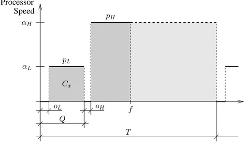
3.2 Energy management scheme . . . 38
3.2.1 Processor model . . . 40
3.3 Optimal speed assignment . . . 41
3.3.1 Average Energy Consumption . . . 41
3.3.2 Finding the minimum energy consumption . . . 46
3.4 Examples . . . 49
3.4.1 Uniform Density . . . 50
3.4.2 Exponential Density . . . 52
3.4.3 Impact of the overheads . . . 53
3.4.4 Idle power . . . 53
3.5 Summary . . . 56
4 Resource Reservations 57 4.1 An introduction to Resource Reservations . . . 57
4.1.1 Temporal isolation . . . 58
4.1.2 Qualitative comparison with Proportional share . . . 59
4.1.3 The CBS class of schedulers . . . 60
4.1.4 Algorithms based on CBS . . . 61
4.1.5 Issues with CBS . . . 62
4.2 The GRUB Algorithm . . . 63
4.2.1 Formal model of the GRUB algorithm . . . 64
4.2.2 Performance guarantees . . . 68
4.3 Coping with short periods . . . 69
4.3.1 The HGRUB algorithm . . . 70
4.3.2 Formal properties of HGRUB . . . 70
4.3.3 Considerations about HGRUB . . . 74
5 The GRUB-PA Algorithm 77 5.1 Introduction . . . 77 5.2 Algorithm GRUB-PA . . . 78 5.2.1 An example . . . 80 5.2.2 Properties of GRUB-PA . . . 82 5.2.3 Discrete frequencies . . . 84 5.2.4 Overhead . . . 86
5.3 Evaluation of the algorithm . . . 86
5.3.1 Comparison with DRA and RTDVS . . . 88
5.3.2 Comparison with DVSST . . . 92
5.4 Implementation and experimental results . . . 92
5.4.1 Test-bed . . . 95 5.4.2 Experimental results . . . 98 5.5 Summary . . . 100 6 Final Remarks 101 6.1 Conclusions . . . 101 6.2 Ongoing work . . . 103
A Supporting Real-Time Applications on Linux 105 A.1 Introduction . . . 105
A.2 Towards a Real-Time Linux Kernel . . . 107
A.2.1 Problems Using Standard Linux . . . 107
A.2.2 Classification of Linux-based RTOSs . . . 108
A.3 Interrupt Abstraction . . . 109
A.3.1 Advantages . . . 112
A.3.2 Limitations of RTLinux and RTAI . . . 112
A.3.3 The Xenomai approach . . . 113
A.4 Making the Kernel More Predictable . . . 114
A.4.1 Reducing Kernel Latency . . . 114
A.4.2 Improving Timing Resolution . . . 115
A.4.3 The PREEMPT RT patch . . . 116
A.4.4 Resource Reservations . . . 117
A.5 Summary . . . 118
List of Figures
1.1 Real-time control system. . . 4
1.2 Distribution of execution times of decoding the Star Wars movie. . . 8
1.3 A GANNT chart describing the parameters of a generic job τi,k. . . 9
1.4 A GANNT chart describing a sequence of jobs τi,k belonging to the same task τi. . . 10
2.1 Normalized power consumption of well-known microprocessors. . . 21
2.2 A GANNT chart describing the generic job τi,k on a DVS processor. . . 24
2.3 Taxonomy of energy-aware scheduling algorithms. . . 26
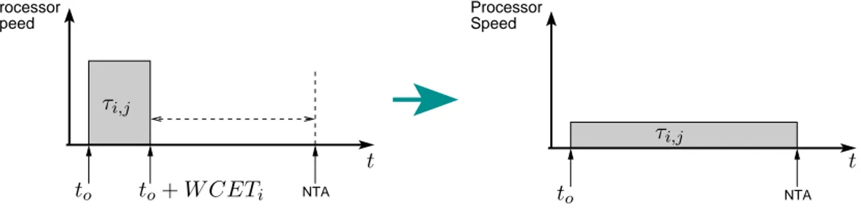
2.4 The Stretching to NTA technique. . . 29
2.5 The energy management scheme of DVS-EDF. . . 34
2.6 The PACE scheme. . . 35
3.1 The energy management scheme used throughout Chapter 3. . . 39
3.2 The active energy EA vs. the computation time c . . . 43
3.3 Eavg for uniform execution times. . . 47
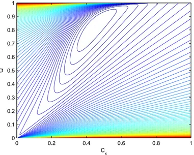
3.4 Level curves of Eavg for exponential p.d.f. . . 47
3.5 The optimal number of cycles in case of uniform density and polynomial power function. . . 50
3.6 Exponential probability density functions. . . 52
3.7 The optimal (Cx, Q) pair as function of the symmetry for exponential p.d.f. 53 3.8 Impact of the time overhead o on the average energy consumption using an exponential p.d.f. with β = −50 and a cubic power function. . . 54
3.9 Impact of the energy overhead e on the average energy consumption using an exponential p.d.f. with β = −50 and a cubic power function. . . 54
3.10 Impact of the idle power on the finishing time using an exponential p.d.f. and a cubic power function. . . 55
3.11 Impact of the idle power on the speed αL using an exponential p.d.f. and a cubic power function. . . 55
3.12 Impact of the idle power on the speed αH using an exponential p.d.f. and a cubic power function. . . 56
4.3 The “Short Period” problem of CBS and GRUB. . . 70
4.4 State transition diagram of HGRUB. . . 71
5.1 State transition diagram of GRUB. . . 80
5.2 An example of schedule produced by GRUB-PA. . . 81
5.3 Energy consumption with WCET/BCET ratio equal to two on a PXA250. . 89
5.4 Energy consumption with WCET/BCET ratio equal to two on a TM5800. . 89
5.5 Energy consumption with WCET/BCET ratio equal to four on a PXA250. 90 5.6 Energy consumption with WCET/BCET ratio equal to four on a TM5800. 90 5.7 Energy consumption with constant average workload on a PXA250. . . 91
5.8 Energy consumption with constant average workload on a TM5800. . . 91
5.9 Energy consumption with variable average workload on a PXA250. . . 93
5.10 Energy consumption with variable average workload on a TM5800. . . 93
5.11 Intrinsyc Cerfcube. . . 95
5.12 Intel PXA250 block diagram. . . 96
5.13 Decompression speed related to processor speed. . . 98
5.14 Current entering in the CerfCube system during the boot. . . 99
List of Tables
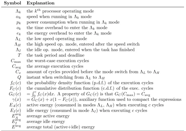
3.1 Glossary and notations used throughout Chapter 3. . . 42
5.1 Operating parameters for the Intel Xscale PXA250 processor. . . 87
5.2 Operating parameters for the Transmeta Crusoe TM5800 processor. . . 88
5.3 Average values of the input current. . . 99
A.1 Interrupt and task latency in the standard Linux 2.4 and in RTAI. All measures are in microseconds. . . 111
A.2 Average and maximum latency values using a standard Linux 2.4.17, the Preemptible Kernel and the Low Latency patches. . . 115
A.3 Latency comparison between Standard Linux, Linux with the PREEMPT RT patch, and Adeos. All numbers are in microseconds. . . 116
Introduction
The number of embedded systems operated by battery is increasing in several application domains [70], from Personal Digital Assistants (PDAs) to autonomous robots, laptop computers, smart phones and sensor networks [35]. The problem of reducing the energy consumed by these systems has become a key design issue, since they can only operate on the limited battery supply. Many of these systems, in fact, are powered by rechargeable batteries and the goal is to extend as much as possible the autonomy of the system. Battery lifetime is a critical design parameter for such devices, directly affecting system size, weight and cost. Battery technology is improving rather slowly and cannot keep up with the pace of modern digital systems. Thus, reducing the energy consumed by these devices is the only way to prolong their lifetime.
In recent years, as the demand for computing resources has rapidly increased, even real-time servers and clusters are facing energy constraints [71, 27]. In fact, the growth of computational speed in current digital systems is mostly obtained by reducing the size of the transistors and increasing the clock frequency of the main processor. Since the power consumption is related to the operating frequency, the net effect is a growth of the energy demand and (as a side effect) of the heat generated [99, 63, 81]. Conventional computers are currently air cooled, and manufacturers are facing the problem of building powerful systems without introducing additional techniques such as liquid cooling [71, 24]. Cooling is a complex phenomenon that cannot be modelled accurately by a simple model [62, 114]. Heat dissipation directly affects the packaging and cooling solutions for integrated circuits. With power densities increasing due to increasing performance demands and tighter packing, proper cooling becomes even more challenging.
Clusters with high peak power need complex and expensive cooling infrastructures to ensure the proper operation of the servers. Not surprisingly, a significant portion of the energy consumed is due to the cooling devices, which may consume up to 50 percent of the total energy in small commercial servers [71, 90]. Thus, electricity cost represents a significant fraction of the operation cost of data centers [24, 27]. For example, a 10kW rack consumes about 10MWh a month (including cooling), which is at least 10 percent of the operation cost [20], with this trend likely to increase in the future. Clearly, good energy management is becoming important for all servers. To better understand the impact of
techniques for reducing power consumption in high-end servers, consider the cost savings that can be obtained by reducing the energy consumed in large web server farms, in terms of air conditioning and cooling systems: reducing the energy consumed by the computing components would impact on the energy consumed by the cooling devices and, in the end, on the total cost of the system.
In order for all these systems to be active for long periods of time, energy consumption should be reduced to an absolute minimum through energy-aware techniques. For this reason, the current generation of microprocessors [93, 131, 58, 57, 59, 60, 55] allow the operating system to dynamically vary voltage and operating frequency to balance com-putational speed versus energy consumption. This technique is called Dynamic Voltage Scaling (DVS) [99] and is used by many energy-aware scheduling policies already proposed in the literature [112, 98, 18, 101, 141].
In real-time systems and time-sensitive applications, however, if this frequency change is not done properly, some important task may miss its timing constraints. The problem is even more difficult considering that in practice most systems consist of a mixture of critical (i.e., hard) and less critical (i.e., soft) real-time tasks. For these reasons, develop-ers typically design these systems so that they provide the highest computational power in any circumstance, in order to guarantee the timely execution of those computational activities that must meet predefined timing constraints. However, peak load conditions rarely happen in practice, and system resources are underutilized most of the time. For example, server loads often vary significantly depending on the time of the day or other external factors. Researchers at IBM showed that the average processor use of real servers is between 10 and 50 percent of their peak capacity [27]. Thus, much of the server ca-pacity remains unused during normal operations. These issues are even more critical in embedded clusters [138], typically untethered devices, in which peak power has an impor-tant impact on the size and the cost of the system. Examples include satellite systems or other mobile devices with multiple computing platforms, such as the Mars Rover and robotics platforms. Some studies have observed that the actual execution times of tasks in real-world embedded systems can vary up to 87 percent with respect to their measured worst case execution times [134].
We believe that the advantages of DVS can be exploited even in real-time systems, through a careful identification of the conditions under which we can safely slow down the processor speed without missing any predefined timing constraint. This way, the reduction of the power consumption does not affect the timely execution of important computational activities. In particular, an energy-aware scheduling algorithm can exploit DVS by selecting, at each instant, both the task to be scheduled and the processor’s operating frequency.
INTRODUCTION
Energy-Aware Scheduling topics. We focus on algorithms for uniprocessor systems, since the lack of optimal scheduling algorithms for real-time multiprocessors makes the problem of creating energy-aware algorithms with high efficiency very difficult.
The main contributions of this thesis can be summarized as follows. We start by studying the problem of energy minimization from an analytical point of view. We propose a novel result in the real-time literature which integrates the concept of probabilistic execution time within the framework of energy minimization. In particular, we find the optimal value of the instant of frequency transition (i.e., transition point) and of the speed assignment in a two-speed scheme where probabilistic information about task execution times is known. Through this study we show that saving energy while still meeting real-time constraints is actually possible. Unlike similar results presented in the literature so far, the optimal values are found using a very general model for the processor that accounts for the idle power and for both the time and the energy overheads due to voltage/frequency transition. Our result represents a net improvement over the sub-optimal mechanism used in the DVS-EDF algorithm proposed by Zhu et al. [43, 141].
This thesis also includes a study about the Resource Reservation technique [104]. In particular, we investigate some anomalies in the schedule generated by the CBS [6] and GRUB [76, 75, 77] algorithms and we propose a novel algorithm, called HGRUB [11], which maintains the same features of CBS and GRUB but it is not affected by the problems described.
Then, starting from the GRUB algorithm proposed by Lipari and Baruah [76, 75, 77], we develop a novel energy-aware scheduling algorithm called GRUB-PA which, unlike most algorithms proposed in the literature, allows to reduce energy consumption on real-time systems consisting of any kind of task — i.e., hard and soft, periodic, sporadic and even aperiodic tasks. With this algorithm we show that saving energy while meeting real-time constraints is possible even in presence of a mixture of hard and soft real-time tasks. The effectiveness of the algorithm is validated through the formal proof of its main properties and through a series of comparisons with the state of the art of energy-aware scheduling algorithms using the RTSim 0.3 [96, 4] scheduling simulator.
Last but not least, we describe a working implementation of the GRUB-PA algorithm in a real test-bed running the Linux operating system and we present a series of experiments to show that the algorithm actually reduce the energy consumption of the system.
The main results of this thesis have been already published at several conferences [111, 112, 110, 107, 78, 11] and on the IEEE Transactions on Computers journal [113], and have been accepted for publication on a special issue of the International Journal of Embedded Systems (IJES) journal [26].
This thesis is organized as follows. In Chapter 1, we introduce definitions and char-acteristics concerning real-time systems as well as the scheduling model that will be used
throughout the rest of this thesis. The interested reader can refer to Appendix A for an overview of some working implementations of real-time operating systems (RTOSs) based on Linux. In Chapter 2, we describe some architectural aspects concerning the DVS technique for CMOS circuits. Then, we propose a taxonomy of energy-aware scheduling algorithms and we provide an overview of the state of the art of the algorithms proposed in the real-time literature. In Chapter 3, we study the problem of energy minimization from an analytical point of view, finding the optimal values of transition point and speed assignments when probabilistic information about task execution times is known. The op-timal values are found using a very general model for the processor that accounts for idle power and for both the time and the energy overheads due to voltage/frequency transition. In Chapter 4, we recall some concepts about the Resource Reservation technique [104] and we propose the GRUB and HGRUB algorithms that effectively solve some drawbacks of the original Constant Bandwidth Server (CBS) algorithm [6]. These algorithms will then be used as basis for our energy-aware scheduling algorithm GRUB-PA, presented in Chap-ter 5, which reduces energy consumption on real-time systems consisting of hard and soft, periodic, sporadic and aperiodic tasks. Finally, in Chapter 6 we state our conclusions, providing an overview of the ongoing and future work.
Acknowledgments
First of all, I would like to thank Jesus Christ (my life and my peace) for making all of this possible.
Thanks with all my love to Giulia, my wife, for her love and her patience during the trips back and forth from the United States.
My special thanks are for my two supervisors, namely prof. Giuseppe Lipari and prof. Susanna Pelagatti, for their precious help and their important suggestions. Working with you was really a honor!
Thanks to Enrico Bini, co-author of Chapter 3 and master of the LaTeX language. Many thanks to prof. Daniel Moss´e, Alexandre P. Ferreira, Kirsten Ream and all the people at the University of Pittsburgh. Studying at Pitt has been a wonderful experience and I hope to have the chance of meet all of you again and soon.
Thanks to prof. Hakan Aydin for his help in the development of the code of the DRA algorithm in the RTSim environment [16, 4].
Thanks also to my colleague Paolo Gai who gave me the exciting opportunity of work-ing at Evidence.
Last but not least, many thanks to Luca Abeni and Michael Trimarchi for their precious teaching about Linux kernel internals.
Chapter 1
Real-Time Systems
This chapter introduces basic terminology, definitions and notation concerning real-time systems as well as the scheduling model that will be used throughout the rest of this thesis. The interested reader can refer to Appendix A for an overview of some existing implementations of real-time systems based on Linux.
1.1
Introduction to Real-Time Systems
Real-time systems are “systems in which the correctness depends not only on the logical result of the computation, but also on the time at which the results are produced” [125, 116]. Thus, a system can be defined real-time if “it produces the results within a finite and predictable interval of time”, which is not necessarily the fastest time possible.
The system controlling the speed of a train is an example of real-time system: once an obstacle has been detected, the action of activating the brakes must be performed within a maximum delay, otherwise the train will crash on the obstacle. Keeping the previous example in mind, a real-time system can be more precisely defined as follows:
Definition 1 [32] A real-time system is a computing system in which computational ac-tivities must be performed within predefined timing constraints.
Typically, a real-time system is a controlling system managing and coordinating the activities of some controlled environment (see Figure 1.1). The real-time system acquires information about the environment through some sensors [35], and controls the environ-ment using actuators. The adjective “real” means that the clock of the environenviron-ment and the clock of the real-time system are synchronized. The environment creates some events, and the real-time control system must respond to these events within a finite and pre-dictable period of time. The interaction is bidirectional, and is characterized by timing correctness constraints: the control — i.e., the reaction to internal or external events — must be done within finite and pre-established delays. Since a real-time system must
Environment Real−time control
Event (Re) action
Figure 1.1: Real-time control system.
provide guarantees about its response times, it must have a predictable and deterministic timing behaviour.
Notice that the concept of “real-time” is not synonymous of “fast”: having the re-sponse of the system within the timing requirements is sufficient. The objective of fast computing is to minimize the average response time of a given set of tasks. The objective of real-time computing, instead, is to meet the individual timing requirements of each task. Rather than being fast (which is a relative term), the most important goal in real-time system design is predictability — that is, the functional and timing behaviour of the system must be as deterministic as necessary to satisfy system specifications. This deter-minism allows to provide timing guarantees about the evolution of the environment. The fastness of the system (i.e., a low latency) remains in any case a desirable feature, since it allows to respond in a short time to events that need immediate attention [116] — fast computing is helpful in meeting stringent timing specifications, but it does not guarantee any predictability.
In the last decades, real-time systems have started to be used in different areas of everyday life. Nowadays, real-time capabilities can be found in several electronic devices, from simple PDAs for audio and video streaming to complex critical systems for the con-trol of nuclear power plants. Examples of use of a real-time system include the concon-trol of laboratory experiments, car engines, nuclear power plants, chemical stations, flight systems, space shuttle and aircraft avionics, robotics and rocket systems [126, 32, 116]. Real-time systems are also widely used in many areas of telecommunications and multi-media, to guarantee timely execution of applications and proper Quality of Service (QoS) to end-users.
1.2. DESIGN ISSUES 5
1.2
Design Issues
Although in the last decades, a strong mathematical theory has been successfully developed to model and formalize the behaviour of a real-time system [126, 32, 79], sometimes the development of such systems is still done in empirical ways, using heuristic assumptions. In other cases, the real-time system is sized according to the worst case scenario, resulting in a partial utilization of the available resources (e.g., the processor).
Some designers consider that a fast enough system is always able to respond in time. If an infinitely fast computer was available, we would not have any real-time problem, because the system would be capable of immediate response to any event, regardless of the current workload. However, even if advances in hardware technology will likely exploit faster processors to improve system throughput, this does not mean that timing constraints will be automatically met. Moreover, we must consider that the greater is the computational power provided by the hardware, the greater is the amount of resources needed. The amount of available computational power, in fact, affects many different aspects of the system, like the cost, the size, the energy consumption, the heat and noise produced and the fault robustness. For instance, the growth of computational power in current microprocessors is mostly obtained by reducing the size of the transistors in order to increase the clock frequency. This leads to both greater power consumption and greater heat production. Heat dissipation directly affects packaging and cooling solutions for integrated circuits, which, in turn, affect the size and the cost of the whole system.
This problem is critical especially in the field of “embedded” systems. These are special-purpose computers part of larger systems or machines that may not be of electronic kind (think, for instance, to the embedded system controlling an automotive engine). Typically, an embedded system is expected to work without human intervention, and it is housed on a single microprocessor board with the programs stored in ROM. In these systems, there is the need of reducing the resources used by the system as much as possible — brute force techniques do not scale to meet the requirements of guaranteeing real-time constraints on embedded devices. For instance, the development of operating systems for embedded devices starting from those for higher level architectures has often collided with the limited number of available resources. In an embedded system, the trade-off between the provided computational power and the amount of resources needed is very important. In particular, parameters like cost, size and energy consumption are decisive factors for the actual usability of such systems. Notice that the cost and the size are often conflicting goals, since the development of smaller devices is typically more expensive. Moreover, in embedded real-time systems there is the intrinsic trade-off between the importance to pursue such aims, and the need to have enough computational power to guarantee the real-time constraints.
re-sources needed to the minimum possible value. During the last decades several formal ap-proaches have been proposed to formalize the behaviour of a real-time system exactly [31]. However, they have been seldomly used in the design of real systems.
Currently, real-time system design is mostly ad hoc. This does not mean, however, that a scientific approach is not possible: most good science grew out of attempts to solve practical problems. For instance, the first flight of the space shuttle was delayed, at considerable cost, because of a timing bug that arose from a transient processor overload during system initialization [125]. The development of a scientific basis for verifying that a design is free of such bugs is clearly necessary.
1.3
Real-Time Operating Systems
Typically, a real-time system is implemented as a set of concurrent tasks that are exe-cuted on a Real-Time Operating System (RTOS). Each task represents a computational activity that needs to be performed according to a set of constraints. The objective of the RTOS is, thus, to manage and control the assignment of the system resources (e.g., the microprocessor) to the tasks in order to meet such constraints.
Definition 2 [3] A real-time operating system (RTOS) is an operating system capable of guaranteeing the timing requirements of the tasks under its control through some hypothesis about their behaviour and a model of the external environment.
“RTOS” is a generic term for a set of operating systems providing some kind of support for real-time applications. There is a wide range of RTOSs, from the small and simple system that fits in few kilobytes of memory and can run on simple processors, to the high-end RTOS providing full graphical user interface and requiring several megabytes of RAM and powerful processors (with MMU, protected mode, etc.).
A real-time system should be flexible enough to react to a highly dynamic and adaptive environment, but at the same time it should be able to avoid resource conflicts so that timing constraints can be predictably met. The environment may cause any unpredictable combination of events to occur, but the real-time system should be carefully built in order to predict the possibility of meeting timing constraints at any time during execution.
Desirable features of a RTOSs are the co-existence of normal and real-time tasks, low latency, and fault tolerant mechanisms [6, 48, 9, 8, 32]. Appendix A explains how these goals can be achieved in Linux in order to create a real-time operating system.
1.4
Real-Time Tasks
Real-time scheduling involves the allocation of system resources to tasks in such a way that certain predefined timing requirements are met. Scheduling has been probably the
1.4. REAL-TIME TASKS 7
most widely researched topic in the real-time literature [126].
Definition 3 [126] A real-time task is an executable entity of work which is characterized, at least, by a worst case execution time and a timing constraint. It denotes a generic scheduling entity, that can correspond to either a thread or a process on a real operating system.
Depending on the type of application, different timing constraints (like the jitter on the initial or the finishing time of execution) can be defined. A typical constraint is the deadline, which is the instant of time the task’s execution is required to be completed. A real-time task must complete before its deadline, otherwise the results could be produced too late to be useful. The deadline is the only timing constraint that we will consider throughout this thesis.
Typically, real-time tasks have a cyclic structure in which they execute some code and then they block waiting for a timer or for a particular event. For this reason, real-time tasks can be well modelled by thinking each task as consisting of a sequential stream of “jobs”.
Definition 4 [126] A job is an instance of a real-time task.
The job is the unit of work, scheduled and executed by the operating system. We say that a job arrives when the task unblocks (i.e., when the task becomes ready for execution), and that the job ends when the task blocks. Jobs of the same task must be executed sequentially — i.e., the concurrent execution of jobs of the same task is not possible.
Typically, tasks have variable execution times between different jobs. The execution time, in fact, depends on several factors like input data, current state of cache and pro-cessor pipeline, etc. As an example, consider the two branches of a typical if-then-else statement, which may have very different computation times.
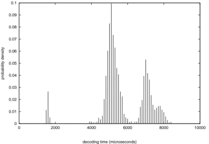
There are many real-time applications in which the worst-case scenario happens very rarely, but its duration is much longer than the average case. Some studies have observed that the actual execution times of tasks in real-world embedded systems can vary up to 87 percent with respect to their measured worst case execution times [134]. An algorithm with highly variable computation time is the decoding of a MPEG frame, where the execution time depends on the data contained in the frames.
The problem of variable execution times is typically handled in the real-time literature by defining a parameter of the task called Worst Case Execution Time (WCET), which represents the maximum possible value that the computation times of task’s jobs can assume. Another parameter, called Worst Case Execution Cycles (WCEC), represents the
0 0.01 0.02 0.03 0.04 0.05 0.06 0.07 0.08 0.09 0.1 0 2000 4000 6000 8000 10000 probability density
decoding time (microseconds)
Figure 1.2: Distribution of execution times of decoding the Star Wars movie.
maximum possible processor cycles required by the task instances, and is typically used when dealing with processors having dynamic speed.
Computing the exact value of the WCET of a task consists on computing the execution time of all the possible paths that the program may follow, then selecting the path with the maximum execution time. This computation is possible only in principle. In practice, the problem is intractable even for deterministic programs: the presence of caches, pipelines, DMA and branch prediction makes the problem of computing a constant execution time very difficult. In fact, although these mechanisms reduce the average execution time of a task, they make much more difficult the estimation of worst case execution times [32]. Moreover, the worst case path may never happen in practice (because not possible). Thus, the value estimated for the WCET in practice is affected by large errors (typically, more than 20 percent [32]). Therefore, an interesting property of the scheduling discipline is the ability of reclaiming resources used by tasks that execute less than their worst case requirements. As we will see in Chapter 5, our scheduling algorithm, GRUB-PA, has such interesting feature.
A more complete and precise information about the behaviour of a dynamic compu-tational activity like a real-time task is the probability density function (p.d.f.) derived by experimental data. Figure 1.2 shows the probability density function of the execution time of the job decoding a frame of the Star Wars movie [32]. The x axis shows the de-coding time (expressed in microseconds) whereas the y axis shows the probability density function. In Chapter 3, we will study the problem of reducing energy consumption in real-time systems where probabilistic information about execution times is known.
1.5. SCHEDULING MODEL 9 ci,j
ri,j si,j fi,j di,j
Di,j 0
ρi,j
t
Figure 1.3: A GANNT chart describing the parameters of a generic job τi,k.
1.5
Scheduling Model
We consider the processor as the only resource shared by a set of real-time tasks, reducing the scheduling problem to the choice of a possible assignment of the tasks to the pro-cessor. Furthermore, we restrict our attention to preemptive uniprocessor systems, with the assumption that processing is fully preemptible at any point. Thus, at any instant of time, the running task is the highest priority active task in the system. If a low priority task is in execution and a higher priority task becomes ready for execution, the former is preempted and the processor is given to the new arrival. This assumption is realistic on modern operating systems like Linux which, with the advent of the 2.6 kernel series, has become a fully preemptive OS [82] (refer to Appendix A.4.1 for more details).
We consider a system comprised of n real-time tasks τ1, τ2,..., τn. We refer to this set of tasks as the task set τ = {τ1, ..., τn}. Each task τi is a sequential stream of jobs (or instances) τi,1, τi,2, τi,3, ..., where τi,j becomes ready for execution (“arrives”) at time ri,j (ri,j ≤ ri,j+1 ∀i, j), and requires a computation time equal to ci,junits of time. Real-time tasks can be well described through a GANNT chart (see Figure 1.3) having an horizontal time axis for each task. The assignment of jobs to the processor is represented by filled rectangular boxes drawn along the axes. Typically, capital letters are used to represent absolute values in time, whereas small letters are used for relative values.
In particular, a job τi,k is characterized by the following parameters:
Definition 5 (Release time) The release (or activation) time ri,k is the instant of time at which the job becomes ready for execution (because it has been activated by some event or condition).
In the GANNT chart the release time is typically represented by an upward arrow (see Figure 1.3).
Definition 6 (Start time) The start time si,k is the time at which the job starts its execution for the first time (i.e., the first time the processor is assigned to the job).
t
ri,1 ri,2 ri,3
ci,1 ci,2 ci,3
fi,1 di,1 fi,2 di,2 fi,3 di,3
Figure 1.4: A GANNT chart describing a sequence of jobs τi,kbelonging to the same task τi.
Definition 7 (Finishing time) The finishing (or completion) time fi,k is the time at which the job actually completes its execution.
Definition 8 (Relative deadline) The relative deadline Di,k is the interval of time job’s execution is required to be completed with respect to its release time. Typically, this is a constant value equal for all the jobs belonging to the same task, and it is called task relative deadline Di.
Definition 9 (Absolute deadline) The absolute deadline di,k is the absolute instant of time by which job’s execution must complete. The deadline is successfully met if and only if fi,k≤ di,k, otherwise it is missed. The job deadline di,j is computed based on the relative deadline: di,j = ri,j+ Di,j.
In the GANNT chart the deadline is typically represented by a downward arrow (see Figure 1.3).
Definition 10 (Computation time) The computation time ci,k is the time required by the processor to complete job’s execution without interruption.
Definition 11 (Response time) The response time ρi,k is the time elapsed from the job release time to the finishing time (ρi,k= fi,k− ri,k).
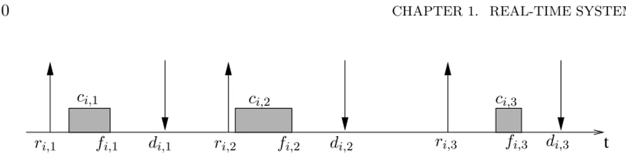
We assume that, for each task, the jobs are executed in FIFO order — i.e., τi,j+1 can start execution only after τi,j has completed. A GANNT chart describing a sequence of jobs belonging to the same task is shown in Figure 1.4.
A task τi is characterized by the following parameters.
Definition 12 (Worst case execution time) The worst case execution time (WCET) of task τi is the worst (i.e., maximum) computation time required by all its instances:
Ci = max
k≥0{ci,k} (1.1)
Definition 13 (Worst case response time) The worst case response time of task τi is the worst (i.e., maximum) response time required by all its instances:
ρi = max
1.6. TASK PERIODICITY 11
1.6
Task Periodicity
Real-time tasks can either be activated by a timer at predefined instants of time or by the occurrence of a specific event or condition [32]. In the former case, an important characteristic of the task is given by the regularity of its activations (i.e., the release times of its jobs) which allows to distinguish between periodic and aperiodic tasks.
Definition 14 Periodic tasks are tasks that are activated (released) at regular intervals of time. In particular, a task τi is said to be periodic if
ri,k+1= ri,k+ Ti ∀k ≥ 1 (1.3) where Ti is the task period. The deadline, if not otherwise stated, corresponds to the end of the period.
Typically, periodic tasks have a regular structure, consisting of an infinite cycle, in which the task executes a computation and then suspends itself waiting for the next periodic activation. A typical periodic task has the following structure:
void * PeriodicTask(void *arg) {
<initialization>;
<start periodic timer, period = T>; while (cond) {
<read sensors>; <update outputs>;
<update state variables>; <wait for next activation>; }
}
A typical characteristic of a periodic task set is a parameter called utilization, which is defined as follows U = n X i=1 Ci Ti (1.4) and represents the computational workload requested by the task set to the processor, assuming that each job executes for its worst-case execution time. This value is typically used to evaluate the schedulability of the task set (see Section 1.9).
Another class of real-time tasks, very similar to periodic tasks, is called sporadic and waits for aperiodic events.
Definition 15 [126] Sporadic tasks are real-time tasks that are activated irregularly with some known bounded rate. The parameter Ti denotes the minimum (rather than exact)
separation between successive jobs of the same task, and is called minimum interarrival time:
ri,k+1≥ ri,k+ Ti ∀k ≥ 1 (1.5) A typical sporadic task has the following structure:
void * SporadicTask(void *) { <initialization>; while (cond) { <computation>; <wait event>; } }
Finally, there is a class of real-time tasks for which it is not possible to set even a minimum interarrival time between two consecutive jobs. This kind of tasks, called aperiodic, does not have any particular timing structure, and typically responds to events that occur rarely (e.g., a state change) or that happen with an irregular structure (e.g., burst of packets arriving from the network).
Definition 16 [126, 32] Aperiodic tasks are real-time tasks which are activated irregularly at some unknown and possibly unbounded rate. For this kind of tasks, the release time of the job τi,k+1 is greater than or equal to that of the previous job τi,k:
ri,k+1 ≥ ri,k ∀k ≥ 1 (1.6)
1.7
Hard and Soft Real-Time Tasks
An inherent characteristic of real-time tasks is that the specification of their requirements includes timing information. A real-time task must complete before its deadline, other-wise the results could be produced too late to be useful. In safety critical applications, for instance, a deadline miss could result in serious consequences for the system. The importance of meeting timing constraints divides tasks into two classes: Hard and Soft real-time tasks.
Hard real-time tasks are those critical activities whose deadlines can never be missed, otherwise a critical system failure can compromise the functionality of the system: failure in meeting timing constraints is a fatal fault and it is as much an error as a failure in the value domain. In particular, a task can be defined as hard real-time when “a deadline miss has the potential to be catastrophic” [29] — i.e., the consequences are incommensurably greater than any benefits provided in absence of failure. This kind of task is typically used to control or monitor some physical device, and a missed deadline may cause catastrophic
1.7. HARD AND SOFT REAL-TIME TASKS 13
consequences. For this reason, hard real-time systems cannot compensate some deadline miss in the worst case with a good performance in the average case, and need an a-priori study to ensure that all deadlines will be met under any possible conditions.
Hard real-time systems are designed under worst-case scenarios, by making pessimistic assumptions on system behaviour and on the external environment. This approach allows system designers to perform off-line analysis to guarantee that the system will be able to achieve the desired performance in all operating conditions that have been predicted in advance. However, the consequence of such worst-case design methodology is that high predictability is achieved at the price of a very low efficiency in resource utilization. Low efficiency means more memory and more computational power which, in turn, affect system costs [31].
Hard real-time tasks are needed in a number of application domains, including automo-tive, air-traffic, avionics, industrial, chemical, nuclear, safety-critical and military controls. Examples of hard real-time systems operated by batteries or by solar cells are autonomous robots operating in hazardous environments, like those sent by NASA for exploring the surface of Mars.
In most large real-time systems, not all computational activities are really hard or critical. For soft real-time tasks, the timing constraints are important but not critical, and the system will still work correctly if some deadline is occasionally missed (it does not compromise the functionality of the system, but there is some kind of degradation of the performance perceived by the user). Typically, the number of missed deadlines is related to the Quality of Service (QoS) provided by the application: a deadline miss does not compromise the correctness of the system, but its QoS degrades. An example is a real-time system guaranteeing a fixed QoS to each user accessing a shared resource. Typical requirements on soft real-time tasks are:
• no more than x consecutive missed deadlines;
• no more than x missed deadlines in an interval of time ∆T ;
• the deadline miss ratio (i.e., percentage or total missed deadlines over the total number of deadlines) not exceeding a certain threshold;
In addition, with respect to hard real-time systems, these systems often operate in more dynamic environments, where tasks can be created or canceled at run-time, or task pa-rameters can change from one job to the other.
Typical examples of soft real-time systems are multimedia (e.g., virtual-reality, interac-tive computer games, home-theaters, audio and video streaming) and telecommunication applications. In the last years, we noticed an incredible growth of interest in supporting multimedia applications (e.g., audio and video streaming) on general-purpose operating
systems. These applications are characterized by implicit, but not critical, timing con-straints, which must be satisfied to provide the desired QoS. A classical example of soft real-time task is an MPEG player. The typical frame rate of a video is 25 Frame Per Second (FPS). If some frame is displayed with a little delay, the user may not even be able to perceive the effect. If frames are skipped or displayed too late, however, the distur-bance becomes evident. Avoiding any delay may involve a costly hardware. Using a soft real-time task, instead, makes possible to allow some occasional delay without affecting the quality perceived by the user.
The distinction between hard and soft real-time systems is useful for a general discus-sion but, in practice, many real systems consist of a mixture of hard and soft real-time tasks. The objective is to guarantee that all hard real-time tasks will always complete before their deadlines and, at the same time, to maximize the QoS provided by soft real-time tasks. Clearly, respecting the timing constraints in such hybrid systems is even more difficult. The problem of mixing hard and soft real-time tasks can be efficiently solved by using the Resource Reservation framework [84, 85, 87, 86] that will be introduced in Chap-ter 4. In ChapChap-ter 5, we will present a novel energy-aware algorithm called GRUB-PA able of scheduling both hard and soft, periodic, sporadic and even aperiodic tasks respecting the timing constraints of each running application.
1.8
Other Constraints
Besides timing constraints (like the deadlines), many further constraints can be defined for real-time tasks executing on a RTOS. In particular, in real RTOSs we often find the following kinds of constraints [31]:
- Precedence constraints. Depending on the specific application, it may be not possible to run the tasks in an arbitrary order (consider, for instance, an assembly line). Therefore, task precedence constraints need to be taken into account. A task τi is said to precede another task τj if τj can only start execution after τi has completed its computation. This kind of constraints can be effectively expressed through a DAG 1.
- Constraints on shared resources. Real-time tasks may require access to certain resources other than the processor, such as I/O devices, networking, data structures, files. When different tasks must access the same resource, it is important to keep the shared resource in a consistent state. If a task is interrupted while it is using a resource, in fact, the resource may remain in an inconsistent state. To solve this
1A Direct Acyclic Graph (DAG) is a pair G = (T, P ) where the vertices in T are tasks and the edges
in P represent the precedence constraints. An edge (τi, τj) means that task τi must be completed before
1.8. OTHER CONSTRAINTS 15
problem the tasks must access the resource in mutual exclusion, so that at one time no more than one task has the permission to use the resource.
The implementation of mutual exclusion policies in real-time systems is difficult because it can lead to a problem known in the literature as priority inversion [117]. This undesired phenomenon creates unbounded delays in the real-time schedule, so that some important task may miss its deadlines.
A priority inversion happens when a high priority task waits for the lock held by a low priority task, which, in turn, has been preempted by a task with intermediate priority. Thus, the high priority task must wait the completion of both the interme-diate priority task (which is blocking the low priority task) and the low priority task (which holds the lock on the shared resource). Waiting for an unbounded time, the high priority task may miss its deadline.
Priority inversion is one of the most critical problems in the development of soft-ware for real-time systems. An example of priority inversion occurred during the Pathfinder mission on Mars. In the operating system (VxWorks) a hidden semaphore shared between two tasks with different priorities was used to protect a pipe. Thus, the higher priority task missed its deadline whenever the task with lower priority was preempted by a task with intermediate priority [105].
The Priority Inheritance and Priority Ceiling protocols, first proposed by Sha et al. [117], solve the problem of unbounded priority inversion [136]. The idea is that the low priority task inherits the priority of the high priority task while holding the lock, preventing the preemption by medium priority tasks. In the Priority Ceiling protocol, for instance, a priority ceiling is assigned to each semaphore, which is equal to the priority of the highest priority task that may use the semaphore. Before any task τi enters a critical section, it must first obtain the lock on the semaphore S guarding the critical section. If the priority of the task τi is not higher than the highest priority ceiling among all semaphores currently blocked by the other tasks, then the lock on S is denied and the task τi blocked. When a task τi blocks higher priority tasks, it automatically inherits the highest priority of the tasks that it is currently blocking. When τi exits a critical section, it resumes the priority that it had before entering the critical section. Finally, a task τi not attempting to enter critical sections can only preempt tasks having lower (inherited or assigned) priority. We have described these two kind of constraints for completeness. However, we will consider timing constraints (in particular, the deadline) as the only constraint in our scheduling model because we consider the processor as the only resource shared among our real-time tasks and we do not impose any precedence order among tasks.
1.9
Taxonomy of Scheduling Algorithms
The real-time scheduling theory addresses the problem of guaranteeing timing constraints in real-time systems.
Definition 17 A scheduling algorithm A is an algorithm that for each instant of time t, selects a task to be executed on the processor among the ready tasks. The scheduling algorithm, applied to a specific task set τ = {τ1, ..., τn}, generates a schedule σA(t), which is a possible assignment of the processor to the jobs.
A scheduling algorithm should be designed in such a way that the timing behaviour of the system is understandable, predictable and maintainable. Scheduling techniques can be classified according to several important characteristics [50] like:
- Adaptation: the ability of the scheduler to detect and adapt to any change in the application behaviour [7];
- Predictability: the ability to analyze the run-time behaviour by, for instance, estimating task’s response time and verifying the timing constraints;
- Complexity: the volume of computation required to make scheduling decisions (e.g., O(n), O(nlogn), O(n2), and so on).
According to these properties, real-time scheduling algorithms can be distinguished into:
- Static or dynamic priority. A static priority, also called Fixed Priority (FP), algorithm assigns static priorities to the tasks off-line, but schedules them at run-time. The schedule itself is not fixed, but the priorities that drive the schedule are fixed [126]. Static algorithms require prior knowledge about the properties of the system, but yield little run-time overhead. Rate Monotonic (RM) and Dead-line Monotonic (DM) are examples of FP algorithms for periodic tasks where the priorities are assigned according to tasks periods and to relative deadlines, respec-tively [116].
Another important class of scheduling algorithms is the class of dynamic priority algorithms, where the priority of a task is computed at run-time and can change during task execution. Dynamic priority algorithms are typically more flexible than static priority ones but may suffer of some drawback, like domino effects in case of overload. Static priority algorithms, instead, are typically more predictable. The most important (and analyzed) dynamic priority algorithm is Earliest Deadline First (EDF) [79], where the highest priority is given to the task with earliest deadline — i.e., the priority of the job is inversely proportional to its absolute deadline.
1.10. SCHEDULABILITY TESTS 17
- Preemptive or non-preemptive. In preemptive schemes, a low priority task may be suspended if a higher priority task is available for execution. Alternatively, in non-preemptive approaches, once started, each task finishes its execution without interruption from other tasks. Clearly, preemptive schemes are more flexible, but they also introduce some time overhead due to context switches. Intermediate ap-proaches, like deferred preemption, exist to avoid preemption during critical time intervals.
- Centralized or distributed. Centralized algorithms are typically used in (uni-or multi-process(uni-or) systems with shared mem(uni-ory, where the communication over-head is negligible. Distributed algorithms, instead, are used in distributed systems where communications take a considerable time, which has to be considered during feasibility analysis.
1.10
Schedulability tests
The goal of system designers is to prove that all tasks (or, at least, a sufficient percentage of them) meet their deadlines.
Definition 18 A task set τ is said to be schedulable by the algorithm A if, in the gen-erated schedule σA(t), every job starts at or after its release time and completes before its deadline:
ri,j ≤ fi,j ≤ di,j ∀i, j (1.7)
In this case, the generated schedule is said to be feasible.
Definition 19 A task set τ is said to be schedulable if there exist some algorithm that produces a feasible schedule.
Definition 20 [126] A scheduling algorithm A is optimal if every task set that is schedu-lable by another algorithm is scheduschedu-lable also by algorithm A.
This definition of optimality is the typical one used in real-time scheduling [126, 32]. Definition 21 A schedulability test for the algorithm A is an algorithm that, given a task set τ = {τ1, ..., τn}, returns YES if and only if the task set is schedulable by A. For periodic tasks, a schedulability test is typically based on the parameter UA
lub (which stands for “utilization least upper bound”), which is an intrinsic characteristic of the scheduling algorithm A: if the total utilization U does not exceed the bound (i.e., U ≤ UA
lub), then it is guaranteed that the task set is schedulable by the algorithm A. When UlubA < U ≤ 1, instead, the task set may or may not be schedulable by the algorithm.
Notice that no existing algorithm can schedule task sets having U > 1, since it means that they are asking for more than 100 percent of processor usage.
In particular, for Rate Monotonic we have that [116]
Ulub= n(21/n− 1) (1.8)
therefore, for large values of n, we have that lim
n→∞Ulub= 0.69 (1.9)
This means that under Rate Monotonic the timing constraints are guaranteed only if the utilization is below a value which is rather far from the optimal total utilization (i.e., U = 1).
An important result in the real-time literature is the theorem stating that for the EDF algorithm Ulub = 1 [79]. This implies the optimality of the EDF algorithm: if a task set is schedulable using some algorithm, then it is schedulable also by EDF. In fact, if U ≤ 1, then the task set is schedulable by EDF, otherwise the task set is not schedulable by any algorithm. In particular, notice that EDF can schedule all task sets that can be scheduled by fixed priority algorithms, but not vice versa. Energy-aware algorithms are typically based on dynamic priorities because they need to exploit system resources up to 100 percent.
1.11
Summary
In this chapter, we introduced the real-time scheduling theory. We explained why such theory is important, and why fast computing cannot guarantee the respect of timing constraints in any circumstance. Moreover, we provided the definitions, the notation and the scheduling model that will be used throughout the rest of this thesis.
In the next chapter, we will see how real-time and energy-saving objectives can be pursued at the same time through the use of energy-aware real-time scheduling algorithms.
Chapter 2
Energy-Aware Scheduling
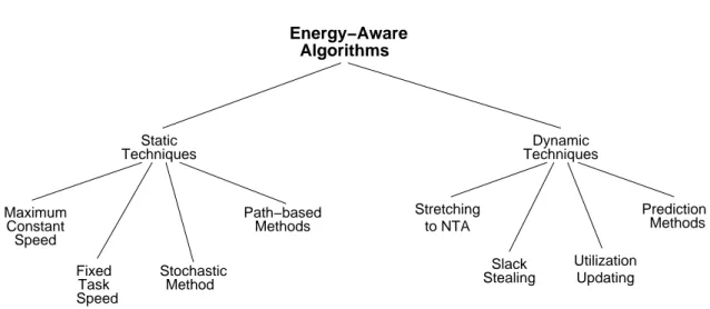
In this chapter, we describe some architectural aspects concerning the Dynamic Voltage Scaling (DVS) technique for CMOS digital circuits. Then, we propose a taxonomy of energy-aware scheduling algorithms and we provide an overview of the state of the art of the algorithms proposed in the literature so far.
2.1
Energy Constrained Systems
The booming market share of embedded systems (like PDAs, autonomous robots, smart phones, sensor networks [35] and so on) has promoted energy efficiency as a major design goal [70]. Many of these systems, in fact, are powered by rechargeable batteries and the goal is to extend the autonomy of the system as much as possible. Battery lifetime is a critical design parameter for such devices, directly affecting system size, weight and cost. Battery technology is improving rather slowly and cannot keep up with the pace of modern digital systems.
In recent years, as the demand for computing resources has rapidly increased, even real-time servers and clusters are facing energy constraints [71, 27]. In fact, the growth of computational speed in current digital systems is mostly obtained by reducing the size of the transistors and increasing the clock frequency of the main processor. As we will show in the next sections, power consumption is related to the operating frequency. Thus, the net effect is a growth of the energy demand and (as a side effect) of the heat generated [99, 63, 81]. Clusters with high peak power need complex and expensive cooling infrastructures to ensure the proper operation of the servers and manufacturers are facing the problem of building powerful systems without introducing additional techniques such as liquid cooling [71, 24]. Moreover, cooling, and hence temperature, is a complex phenomenon that cannot be modelled accurately by a simple model [62, 114].
In order for these devices to be active for long periods of time, energy consumption should be reduced to an absolute minimum through energy-aware techniques. At the same
time, however, it is important to guarantee the timing constraints of the real-time appli-cations. Many of these devices, for instance, use a soft real-time computation to ensure a proper Quality of Service (QoS) in telecommunications or in multimedia applications.
Irani et al. [62] wrote a general survey about the current research on several algorithmic problems related to power management (cooling of microprocessors included).
One of the most energy consuming resources in both embedded and high-end machines is the main microprocessor. For this reason, modern processors usually support several operating states with different levels of power consumption [93, 131, 58, 57, 59, 60, 55]. These operating states can be broadly categorized as
- active, in which the processor continues to operate, but possibly with reduced per-formance and power consumption. Processors might have a range of active states with different frequencies and power characteristics;
- idle, in which the processor is not operating. Idle states vary in both power con-sumption and latency for returning the processor to an active state.
2.2
Dynamic Voltage Scaling
2.2.1 CMOS Microprocessors
Nowadays, most digital devices are implemented using Complementary Metal Oxide Semi-conductor (CMOS) circuits. Power consumption of this kind of circuits can be modelled accurately with simple equations [63, 99, 50, 70]. Like in other kind of circuits, in CMOS circuits power consumption can be splitted in two main components:
PCM OS = Pstatic+ Pdynamic (2.1) where Pstatic and Pdynamic are the static and dynamic components of power consumption, respectively.
In the ideal case, CMOS circuits do not dissipate static power (i.e., Pstatic = 0) since, in steady state, there is no open path from source to ground. In reality, bias and leak-age currents through the MOS transistors cause a static power consumption which is a (usually) small portion of the total power consumed by the circuit.
Dynamic power consumption in CMOS circuits is dissipated during the transient be-haviour (i.e., during switches between logic levels). Every transition of a digital circuit consumes power, because every charge or discharge of the digital circuit’s capacitance drains power. Dynamic power consumption is equal to
Pdynamic= M X k=1
2.2. DYNAMIC VOLTAGE SCALING 21 10 20 30 40 50 60 70 80 90 100 20 30 40 50 60 70 80 90 100 Power Consumption (%) Frequency (%) Intel PXA 250 Intel PXA 255 Intel PXA 27x Intel Pentium M Transmeta Crusoe 5800
Figure 2.1: Normalized power consumption of well-known microprocessors.
where M is the number of gates in the circuit, Ck is the load capacitance of the gate gk, fk is the switching frequency of gk per second, and VDD is the supply voltage.
If we assume that the dynamic component is the most dominant one [70], we can associate a power consumption
PCM OS ∝ f · VDD2 (2.3) to the clock frequency f of the microprocessor, as done in [50, 99, 63]. Although not exact, this is the most used model in the real-time literature for the evaluation and the comparison of energy-aware scheduling algorithms and, if not otherwise stated, it is the model that we will assume throughout this thesis. In Figure 2.1, we show the normalized value of the power consumption of some well-known industrial microprocessors. The resulting values have been obtained by applying Equation 2.3 to the values taken from the processors datasheets [130, 131, 58, 57, 59, 60, 56].
Notice that, although the static power is today about two orders of magnitude smaller than the total power, the typical chip’s leakage power increases about five times each generation, and it is expected to significantly affect, if not dominate, the overall energy consumption in integrated circuits. Even if leakage power can be substantially reduced by cooling, this model of the power consumption may be not suitable for next-generations microprocessors [50]. For this reason, in Section 3.2.1, we will introduce a general model for the processor power consumption which considers each mode as a separate entity, and does not assume any relationship among the energy consumption of each level.
2.2.2 Processor Speed
For many applications, the microprocessor is the bottleneck of the system and the main used resource, therefore the assumption that the speed of the running task corresponds to the speed of the processor is quite natural. Thus, when considering the relationship between the microprocessor frequency and the task computation time, we can make the (worst-case) assumption that the number of processor cycles required by the task is con-stant (i.e., independent of the processor speed α) and that a change of the processor frequency does not affect the worst case execution cycles (WCEC) of the task. This assumption is also justified by the experiment described in Section 5.4.2, showing some experimental results on a real test-bed embedded system.
However, if we want a more accurate model of the system, we must consider that the processor is not the only resource involved in the computation: even very simple appli-cations need to access some peripheral (like memory, disk, network card, etc.) through an external bus. Bus frequencies generally diverge from internal processor frequencies, and they do not scale at the same rate as processor does. Since bus access time often limits the performance of data-intensive applications, running the task at reduced proces-sor frequency has a limited impact on performance. This makes the assumption of the task speed corresponding to the processor speed a worst-case model. In particular, this assumption holds only for systems where the memory latency can scale with processor frequency (mainly, systems with on-chip memory). In contrast, for a system where the memory latency does not scale with processor frequency (systems with dynamic memory and memory hierarchies), the WCEC of a task does not remain constant when the pro-cessor frequency scales. In these systems, in fact, there is a constant access latency for memory references, and an increase of the processor frequency increases the number of cycles required to access the memory. Of course, this effect can be relieved using good caches. However, even if we do not assume perfect caches, it is possible to extend the model accounting for the total number of cache misses for the task.
Recently, some frequency models to express WCEC bounds as parametric terms whose components are frequency-sensitive parameters have been proposed in the literature [115, 25]. In these models, cycles are interpreted in terms of the processor frequency, whereas memory accesses are expressed in terms of the memory latency overhead due to the external bus speed. Essentially, the execution time Ci of task τi is splitted into two components:
Ciα= Ci
α + mi (2.4)
where α is the processor speed (expressed in cycles per second, and typically comprised between 0 and 1), Ci (expressed in processor cycles) scales with the clock frequency, and mi (expressed in seconds) does not scale.
2.2. DYNAMIC VOLTAGE SCALING 23
Clearly, the amount of computation time that varies with the processor frequency depends on the particular task and can be different for tasks running on the same system. This more accurate model has been described for completeness, but it will not be used in the rest of this thesis. In fact, we are not interested in an accurate model of the task speed, but rather in a comparative analysis among different energy-aware algorithms.
2.2.3 The DVS Technique
From Equation 2.3, it follows that reducing VDD is the most effective way to lower the power consumption. This technique is known as Dynamic Voltage Scaling (DVS). Many modern processors [93, 131, 58, 57, 59, 60, 55] can dynamically lower the voltage to reduce the power consumption. Unfortunately, a reduction of the power supply voltage causes an increase of the circuit delay. In turn, the propagation delay restricts the clock frequency of the microprocessor: the processor can operate at a lower supply voltage, but only if the clock frequency is reduced to tolerate the increased propagation delay. Thus, in most cases, when reducing the supply voltage it is necessary to lower also the operating frequency (i.e., the microprocessor speed). As a consequence, all tasks will take more time to be executed. In real-time systems, if this frequency change is not done properly, the timing requirements of the application cannot be respected. Therefore, the advantages of the DVS technique can be exploited in real-time systems only after a careful identification of the conditions under which we can safely slow down the processor without missing any deadline (for hard real-time tasks) or missing a limited number of deadlines (for soft real-time tasks). This way, the reduction of the power consumption does not affect the timely execution of important computational activities. In particular, an energy-aware scheduling algorithm can exploit DVS by selecting, besides the task to be scheduled, also the processor’s operating frequency at each instant of time. The problem becomes more difficult in systems with a combination of hard and soft, periodic and aperiodic real-time tasks.
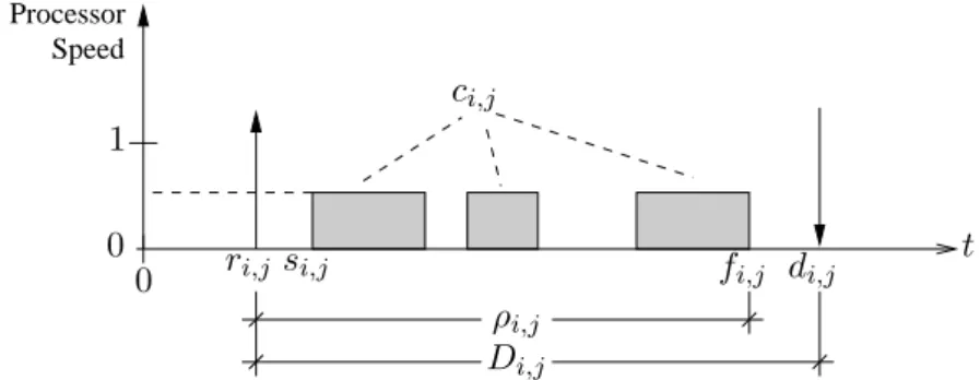
Real-time systems with variable speed are still described using GANNT charts as shown in Figure 2.2. This figure is similar to Figure 1.3, with an additional vertical y axis which represents the current speed of the processor. Thus, the height of the filled rectangular box representing the assignment of the job to the processor specifies the speed at which the job itself is executed. The speed of the processor is typically represented using the α symbol [98, 43, 25]. For an explanation of the parameters shown in the figure, refer to Section 1.5.
Timeliness and energy efficiency are often seen as conflicting goals. Thus, when de-signing a real-time system, the first concern is usually time, leaving energy efficiency as a hopeful consequence of empiric decisions. However, some papers presented in the real-time literature [17, 18, 112, 141] have shown that both goals can be achieved at design time.