UNIVERSITÀ DI PISA
Facoltà di Ingegneria
Corso di Laurea in Ingegneria delle Telecomunicazioni
Tesi di Laurea Specialistica
Distributed PCA-based anomaly detection in
telephone networks through legitimate-user
profiling
Relatori:
Prof. Stefano Giordano
Ing. Rosario G. Garroppo
Ing. Christian Callegari
Ing. Maurizio Dusi
Candidato: Christian Vitale
3
4
Table of contents
1 Introduction ….………... 7
2 Security issues in a telephone network ……... 15
2.1 Attack classification……… 15
3 PCA for telephone anomalies ……….. 22
3.1 Principal Component Analysis………. 23 3.1.1 Computation of the Principal
Components………. 25 3.1.2 Mapping the data-samples………... 28 3.2 Dataset Description……….. 32 3.3 Telephone Network: application scenario… 34 3.4 Centralized PCA-based anomaly detection
technique………. 37 3.4.1 Parallelization of the computation of the
PCs………. 38 3.4.2 Anomaly detection stage………. 43
5
4 A distributed PCA-based approach in a
telephone network…... 44
4.1 Pollution of the legitimate-profile………… 44 4.2 The methodology………. 46 4.2.1 Probe side: PCA analysis…………. 47 4.2.2 Central node side: gathering the
legitimate user profile………... 48 4.2.3 Community check: the Joining
Phase………. 55 4.2.4 Probe side: Anomaly detection……. 60
5 Experimental Results………... 62
5.1 Numerical evaluation of the Distributed anomaly detection technique……… 63 5.1.1 Probe side: PCA analysis…………. 63 5.1.2 Gathering the legitimate profile…… 67 5.1.3 Anomaly detection stage…………... 72 5.1.4 The importance of the joining phase. 80 5.2 Comparison against the centralize
approach……… 83 5.2.1 Profiling of the anomalous users…... 84 5.2.2 Stability of the legitimate user
6
5.3 Changing the number of probe………. 95
6 Conclusion………... 99
7
1
Introduction
The continuous growth of the Internet, and its increasingly presence as a means for Telecommunication, makes progressively relevant the identification of anomalous behaviors in network traffic. This research topic is becoming important also in telephone networks, due to the fact that the use of VoIP (Voice over IP) technologies is more and more widespread today. Indeed, beyond the remarkable advantage of lower costs and the access to a large number of web-based services, such as video communications or text-messaging chat, many IP-based threats that plagued Internet users start to be directed to the VoIP services. It is really easy to foresee that VoIP users are already targets of attacks such as Telemarketer activity, Eavesdropping, Identity theft and Denial of Services.
To reveal this type of attack, several intrusion detection systems have been developed over time, even in telephone context. An intrusion detection system can follow two different approaches: signature-based, where the system identifies patterns of traffic or application
8
behaviors recognized to be malicious; anomaly detection-based, where the system gathers a “normal” baseline through statistical analysis and compare the activities within the network of application with it. For this reason, this second type of intrusion detection system is in general preferred when the working scenario is unsupervised, i.e. there is no a priori knowledge of the normal or the anomalous behavior of the traffic.
As we can see in the following chapter, in a VoIP environment, or more generally in a telephone network, the intrusion detection techniques can exploit several informations to identify anomalous behaviors. For this reason, they can work both at a fine-grained level, evaluating if a given call or the behavior of a user is anomalous or not, both looking to the general behavior of the user and analyzing the statistics of its calls.
In general, in the first case we talk of intrusion detection techniques[1] that can be found at each level of the telephone network, from the backbone to the end-user systems, because they are able to identify anomalous behaviors looking to the management plane, for example the header of the Session Initiation Protocol (SIP)
9
packets, but also to the data plane, for example the Real Time Protocol (RTP) packets.
In general, in the second case we talk of unsupervised anomaly detection techniques[2] that rely on a central node able to collect raw data regarding the calls of the phone users, to gather the description of a legitimate user profile, and to perform anomaly detection based on it. For example, it is possible to define the set of behaviors exhibited by the majority of the phone users as the legitimate profile. In this kind of intrusion detection systems, there are various types of data used to analyze the statistics of a phone call but one of the most immediate way to get this information is through the Call Detail Records (CDRs). Indeed, the CDRs are labels used for billing purpose and they contain general information for each call, such as the source and destination phone number and the call duration.
This work represents mine contribution to the research in this field and is the result of a six-month internship at the Network Laboratories of NEC, Heidelberg (Germany). The work was performed thanks to the collaboration of my local supervisor, Dr. Maurizio Dusi, and my referent for University of Pisa, Dr. Christian Callegari.
10
In this thesis we propose a novel anomaly detection technique that tries to solve two of the main drawbacks of having a central node responsible for the anomaly detection stage:
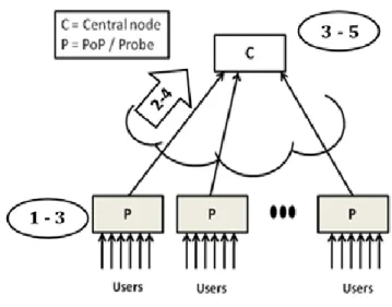
1. it does not allow to take advantage of the probes already distributed over the network. For scalability reason, telephone networks are commonly designed according to a hierarchical topology[15], where Points of Presence (PoPs) are the bridge between end users and the overall network infrastructure, and each PoP is already able to collect and to process the information regarding the part of the network they are able to see.
2. anomalies that are localized on few PoPs can pollute the description of the legitimate profile when aggregated together, thus affecting the classification decision of the central node. For instance, if a certain attitude is sparse over few PoPs, contribute to form the legitimate profile when data are considered as a whole, since the aggregation hides the sparseness of the activity.
11
To overcome these issues, our methodology allows operators to gather an unsupervised description of a pollution-free normal user behavior of their network and subsequently to perform distributed anomaly detection, thus taking advantage of the topology of the network itself. The methodology gathers the behaviors of each users analyzing them during a specific interval of time, through general statistics obtained from the CDRs of their calls and, in the processing stage, it combines Principal Component Analysis (PCA), a well-known method for network anomaly detection[3][12][13], with Agglomerative Hierarchical Clustering (AHC), a method used in the complex network field to identify community within a network[4].
In mathematical terms, through PCA it is possible to represent a high dimensional space, given in our case by different statistics describing the telephone activities of each user, in a new reference system. The dimensions of the new reference system, called typically Principal Components (PCs), are a linear combination of the original ones, and are defined in such a way that the first one points towards the direction that account for as much of the variability in the data as possible, and each
12
succeeding ones points towards the direction of the highest variability possible, under the constraint that it be orthogonal to each preceding dimension. With such a transformation of the original reference system, the first PCs obtained are able to collect most of the variance within the dataset and to describe the “common” behaviors within the network. For this reason, the first PCs are the descriptors of the so-called normal subspace and the descriptions of users well approximated by only means of them represent the legitimate profile. Conversely, descriptions of users that also need the remaining components, that describe the so-called anomalous subspace, represent rare behaviors within the network and they can be labeled as anomalous.
The idea is to let each PoP perform PCA on its portion of users, gathers the description of the normal subspace and send it to a central node. The central node then applies an AHC algorithm to identify communities of probes with similar description of the normal subspace and select the community that contains the legitimate profile. Eventually each PoP exploits such profile to perform PCA-based anomaly detection on its own set of users.
13
To evaluate the effectiveness of the proposed methodology, we compare it against a classical application of the PCA on a given dataset, i.e. a centralized approach where a central node performs PCA on the whole set of users present within the network. Experimental results show that our distributed technique has several advantages over the centralized approach. First, it is able to point out behaviors of users that are widespread within PoPs, whereas in the centralized approach such behaviors affect the computation of the normal subspace. Second, our approach leads to a profile which is stable over time.
In more detail our contribution is:
a parallelization of the computation of PCs on a hierarchical topology;
a distributed technique for PCA-based anomaly detection;
design of an unsupervised mechanism for automatically gathering the profile of legitimate phone users;
14
profiling of actual phone users labeled as anomalous.
The remainder of the thesis is organized as follows. In Chapter 2 we present the possible attack that can be brought to a telephone network and in general how they can be faced exploiting the available information. In Chapter 3 we present a classical application of the PCA with an example of how the computation of the PCs can be parallelized, exploiting the hierarchical topology of a telephone network. In Chapter 4 we present our technique in detail, showing the exchange of messages needed to make it work. In Chapter 5 we present experimental results obtained with our technique in several weeks of real telephone traffic and a comparison with the results obtained with the centralized approach. In Chapter 6 we present our conclusions and a possible application of our technique in a network where more than one operator is present.
15
2
Security issues in a telephone
network
The typical flexibility of VoIP solutions also creates, in addition to obvious advantages as outlined above, serious security problems for communication systems that employ it. Since VoIP is directly connected with the data network, bringing an attack is much easier than it was in the traditional telephone network.
Over time, the scientific community has listed several possible attacks towards VOIP or classical telephone architecture. A complete overview can be found in [5]. Below we provide the more important set of these attacks, showing which of them can be pointed out observing the general behavior of a user through a statistical approach.
2.1
Attack classification
The threats that may be brought towards phone architectures may be divided into using 5 basic groups:
16
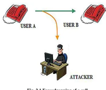
Eavesdropping: the attacker can monitor and intercept the entire signaling and/or the flow of data two or more phone users exchange.
The attacker, however, cannot change them. In the PSTN, this type of attack was only possible with a tap in the terminal user. With VoIP, it is possible to bring it with success if you have easy access to the Internet and appropriate tools. This type of attack, as well as the obvious invasion of privacy, can lead to the interception of sensitive information, ranging from simple e-mail address, stolen to be used in a
17
following attack of SPAM, to the number of credit card or bank account.
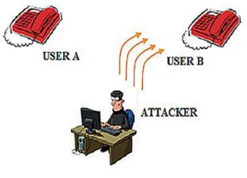
Interception and Modification Threats: in this case, the attacker is also able to change the signaling or the data flow. The attacker is able to interpose himself on calls routed to other telephone users (man in the middle attack), or modify the signaling so that the communication is supported with a degraded QoS.
Fig. 2.2 Men in the Middle attack
Abuse of Service threats: this attack is used to commit fraud or to avoid paying certain telephone
18
services. Indeed, the attacker tries to steal the identity of someone else and let them pay the consequences of his behavior. The identity theft is also used by spammers, in order to avoid some of the prevention technique adopted from telephone network.
In general this type of attack especially plagues VoIP users and is difficult to prevent only looking to the general behavior of the users. Given the type of anomaly detection technique we are proposing, this type of attack is out of the scope of this thesis. Otherwise, these threats are faced by the use of security software tools such as:
Authentication: is needed to understand who the sender of a specific call or packet is. Authentication can take place between different entities or end-to-end.
Encryption: is needed to protect the content of packets from being read by other parties than the ones which are supposed to be their receiver. Encryption follows the same paradigm as authentication, and can be done between two gateways in a tunneling mode, or directly on an end-to-end basis.
19 The remaining groups of attacks are:
Interruption of Service: this type of attacks tries to compromise the availability of a given service, and it can be brought in several ways: sending invalid request so complex which may have the effect of a sharp slowdown or even a crash by a Proxy Server; sending a huge number of requests from a single entity of the telephone network (Denial of Service attack) or from more points at the same time (Distributed Denial of Service), saturating the resources available at a Proxy Server or an endpoint; trying to redirect a call that already exists towards a different endpoint or Proxy Server or to tear it down, sending a BYE or CANCEL request.
20 Fig. 2.3 DoS attack
Social Threats: among other type of attacks, there belongs the activity of telemarketers, where malicious user tries to deliver unsolicited, lawful or unlawful content regarding product or services. This type of SPAM is already present in the traditional PSTN network, but can be potentially more dangerous in VoIP architecture. Indeed, a telemarketer as to face considerably reduced cost in order to make such calls, both in the method by which these calls are placed (a simple software), both in the material costs of the calls themselves (they can exploit flat rates).
A statistical approach, like the one we are proposing in this work, is able to face this last categories of attack
21
thanks to the fact that the activities of such malicious users is significantly different from the common behavior of a normal user. For example, analyzing the incoming and outgoing calls of a user which is carrying out a DoS attack, we would find subsequent short or unestablished placed calls and almost no received calls and it is easy to predict that this is not the normal usage of a telephone.
22
3
PCA for telephone anomalies
When we are searching for an anomalous behavior within the network, we are probably dealing with a huge amount of data-samples described by multivariate features, even if these anomalous events occur infrequently. For this reason, defining a representative normal behavior is challenging and this boundary between normal and outlying behaviors, typically not precise, keeps evolving. With in mind the possible attacks we can face applying an anomaly detection technique, in this chapter we introduce a statistical tool able to express the data in such a way to highlight their similarities and differences, to reduce the dimensionality of the original dataset without much loss of information and to adapt itself to the work conditions: this software tool is the Principal Component Analysis (PCA).This technique is the core of the methodology we propose in this work.
23
3.1
Principal Component Analysis
PCA is a coordinate transformation method that maps measured data onto a new set of axes, the Principal Components (PCs). Each component has the property that it points in the direction of maximum variation remaining in the data, given the energy already accounted for in the preceding components[6].
As such, the first principal component captures the total energy of the original data to the maximum degree possible on a single axis. The next succeeding components then capture the maximum residual energy among the remaining orthogonal directions. In this sense, the axes of the new reference system are ordered by the amount of energy in the data they are able to collect. But how is it possible to compute these Principal Components? In Figure 3.1 we show a two dimensional dataset and the representation of the eigenvector of the covariance matrix C of the dataset itself:
24
Fig. 3.1 Application of PCA to a 2-D dataset
It is possible to see that the plot of data has quite a strong pattern. The two features do indeed increase together. The covariance matrix of such a dataset show strong cross-correlation between the features, and, accordingly, the representation of the eigenvectors of the covariance matrix provide us with information about the patterns in the dataset itself. As we can see from the blue lines, the first eigenvector goes through the middle of the points, like drawing a line of best fit. That eigenvector is showing how these two features are related along that line. The second eigenvector shows the other, less important, pattern in the data, that all the points follow the main line, but are off to the side of the main line by
25
some amount. So, by this process of taking the eigenvectors of the covariance matrix, we have been able to extract lines that characterize the data, i.e. the Principal Components.
Generalization to n-dimensions, as in the case of the dataset we will use in our context, it is not easy to represent in the same graphical way, but works following the same principle.
3.1.1 Computation
of
the
Principal
Components
Shifting from the geometric interpretation to a linear algebraic formulation, the computation of the Principal Components starts from the evaluation of a dataset. Each data-sample of this dataset is described by several dimensions, where each dimension represent a particular feature with which we evaluate the behavior of the data-sample itself. For example, in a telephone network each data-sample can be a phone user, and each feature can be a statistics collected in a particular interval of time regarding the use of the phone he has. A possible feature can be the number of calls placed in the period under
26
analysis, or their average duration. Given this assumption, the description of the whole dataset is done through a matrix Q, where each row represents a phone user and each column represents a feature.
In a general case, the dataset Q is:
where X is the number of data-samples in the dataset and
N the number of features used for their description.
The PCA is applied to the matrix Q and, as we have shown in the preceding sections, transform in a new reference system the features used to describe each data-sample. The obtained PCs are a linear combination of the original axes, and are ordered by the quantity of dataset’s energy they are able to collect. Starting from the dataset
Q, it is possible to compute the PCs following two
different approaches: the covariance method and the singular value decomposition.
Since we will deploy PCA in a distributed environment, we only describe the covariance method. Indeed, it is possible exploit the different PoPs already present in a
27
telephone network, as shown in [7], through the covariance method, parallelizing the computation.
With this method, the computation of the Principal Components is performed through the following steps: 1. Computation of the empirical mean of each column:
at the end of this step, µ is a 1×N row vector.
2. Subtraction of the mean from the correspondent column:
where h is a column vector X×1 of 1’s and B at the end of the step is an X×N matrix.
3. Computation of the empirical covariance matrix of B:
28
4. Computation of eigenvalues v and eigenvectors g of the covariance matrix C. The number of features used, and accordingly the dimensionality of C, can be at most in the hundreds, and any method we choose to evaluate the eigenvector and the eigenvalues make this step less computationally heavy compared to the preceding ones. Indeed in that case we are dealing with matrices large proportionally to our dataset. 5. Sorting the eigenvectors g by the decreasing order of
the correspondent eigenvalues, i.e. the quantity of energy of the dataset they are able to collect. V and G store the eigenvector and the eigenvalues in the new order.
V represents the new basis for the starting matrix B, and
its columns are the Principal Components we are searching for, ordered by the energy of the dataset they are able to collect.
3.1.2 Mapping the data-samples
Given the new reference system, expressed with the matrix V, it’s possible to map all the data-samples in the new reference system through the following equation:
29
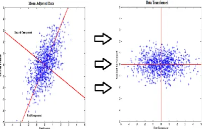
where each row of B’ represents the data-samples in the reference system described by the Principal Components. For example, a final result can be the one shown by Fig.3.2:
Fig. 3.2 Mapping of Data-samples through PCA
If it is possible to find a pattern within the dataset, the first Principal Components can represent each data-sample with a small loss of information because they are able to collect almost the entire energy within the dataset. The pattern shared by the majority of the data-sample is the common behavior of the network, and for this reason,
30
the first PCs are what we claim to be the legitimate profile.
This is the case of the preceding picture, where a single PC is able to characterize the whole dataset. The subspace obtained from the first PCs is also known as the normal subspace. Conversely, a data-sample that has a different behavior from the pattern described by the normal subspace needs also the last Principal Components to be well characterized. The subspace described from these PCs is also called the anomalous subspace.
From this sentence, it follows a way to identify data-samples that acts as outliers. In literature, the error made approximating data-samples with a small number of PCs is called Squared Prediction Error (SPE) and represents their energy into the anomalous subspace. For this reason, the SPE discriminate if a data-sample follow or not the pattern described by the normal subspace. If we use the matrix PC to contain the first P Principal Components, the SPE can be evaluated with the following equation:
31
where PC is an N×P matrix. Using a dataset with the subtraction of the averages of each column is a fundamental part to minimize the SPE.
In previous work where Principal Component Analysis was employed, the tests used to choose the number of PCs that describe the normal subspace were quite different. Among several other tests we have tried[11], such as the Cattel’s Scree Test, the empirical 3 method proposed by Lakhina in [3], the Humphrey-Ilgen parallel analysis and the Broken Stick method, in this section we present the only one that had successful results in our context: the “Cumulative percentage of Total Variation[6]”. The chosen method computes the cumulative percentage of energy contained within the first P eigenvectors with the following equation:
(remember that G contains the value of the ordered eigenvalues, corresponding to the variance collected within the correspondent PC). The number of PCs of the normal subspace is the first P able to collect at least a
32
fixed percentage of the total. In our methodology we set this percentage with a Montecarlo simulation[14] to a 95% value.
3.2
Dataset Description
Thanks to the collaboration with a small European telecom operator, we had the possibility to evaluate the application of PCA in a telephone environment over a dataset composed by 30 millions of calls, collected in a period of five consecutive weeks. In average, we obtained 148K active users each day. The calls were in form of anonymized Call Detail Records (CDR), whose structure is represented in Fig. 3.3.
Fig. 3.3 Call Detail Records
For each call, a CDR contains information such as the source and destination phone number (at least one of the interpreter of each call was an user of the operator that collected the calls), the time the call started, the call duration as well as the cause code or response code, which indicates whether the call was established or if an
33
error occurred. Even if CDRs were from VoIP as well as PSTN networks, this field was given accordingly to SIP reply codes[8].
In our analysis, we interpreted each replay code as a particular status for the correspond call:
Call Status Reply Code
Normal 200,408,486
Suspicious 4XX
Network error 5XX,6XX
We considered a call ending as normal if the code was successful, if the called user did not answer in time or was already busy in a conversation. We considered a call ending as suspicious if there was any other client failure. We considered a call ending with network error if there was a server or global failure in the network.
In our trials, for each day, CDRs were grouped by users and we evaluated the behavior of each user extracting the following N=10 features:
number of calls: placed and received;
number of established calls: placed and received (i.e., calls with a duration greater than zero);
34
number of calls suspicious and with network errors;
number of distinct callers and distinct callees: total and on established calls only.
These features were inspired by previous works on analysis of phone data[9]. The reason behind considering a per-user set of features lays in the fact that our goal was to identify users responsible for anomalous calls rather than in detecting the anomalous calls itself. Under this respect, we believed that the choice of an observation window of one day was a reasonable trade-off between the promptness of the anomaly detection mechanism and the ability to gather user’s behavior with respect to the chosen features.
3.3
Telephone
network:
application
scenario
Telephone networks commonly follow a hierarchical topology, where users connect to the network through Points of Presence and interconnecting switches ensure the communication between PoPs. In Fig.3.4 can represent a possible infrastructure of a telephone network.
35
Fig. 3.4 Possible Topology of a Telephone Network Each PoP is in charge for a specific geographical area and for a set of users which is almost stable over time. This topology allows scalability as the number of users and the volume of traffic within the network increase. In general, even if in the network there are already probes with a partial visibility of the network itself, an anomaly detection technique relies on a central node that collects all the information needed, and directly applies the detection of the anomalous traffic to the raw data. This solution suffers of different drawbacks:
it does not exploit the PoPs already present in the network;
36
requires the transport of a huge and sensitive amount of data through the network;
presents a single point of failure which can become itself target of attacks.
With the assumption that the PoPs just mentioned in a telephone network are able to collect the CDRs both for the incoming and outgoing calls, regarding the set users of their telecomm operator they are in charge of, we present in the following sections two different application of Principal Component Analysis in a telephone environment: an anomaly detection technique that exploits the different PoPs to parallelize the computation of PCs, but still centralizes the raw data and the identification of the anomalous users; our anomaly detection technique, where a PoP that observes traffic of its users and records information about their calls, identifies directly the anomalous users, only receiving the description of the normal subspace of the other probes within the network from a central orchestrator. With our solution we solve part of the problems a centralized technique has. Indeed, we avoid the transportation of the raw data within the network, we exploit all the present
37
PoPs and we distribute the decision over the behavior of the single user, reducing the importance of the central node in the anomaly detection architecture.
3.4
Centralized
PCA-based
anomaly
detection technique
As we have seen in the preceding sections, Principal Component Analysis is able to point out data-samples that do not follow the general behavior of the dataset, i.e. what we claim to be the legitimate user profile.
In the first approach we propose, we apply the PCA in a central node to a matrix Q where each row represents one of the user present within the entire network, and each column is one of the feature we extracted from the CDRs following the process described in section 3.2.
38
3.4.1 Parallelization of the computation of
PCs
Gathering the Principal Components of a matrix like Q (on average in our context a 150K×10 matrix) is computationally heavy due to the calculation of its covariance matrix. For this reason, even if the decisions are taken centralizing all the information from the probes, we found interesting to parallelize the computation of the covariance matrix, thus of the Principal Components. As we said before, the empirical covariance matrix of a generic array Q in general can be computed through the equation:
where X is the number of row of Q and µ is an arrow vector containing the averages of the columns of Q. Following what we found in [7], it’s possible to gather the same results with the subsequent steps:
1. Evaluation of the number of row (X) and of the averages (µ) of the columns of matrix Q.
39
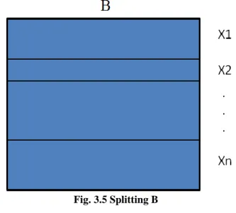
2. Horizontal split of the original matrix Q into n subsets. It’s not important that the subsets obtained have the same number of row, as we can see from Fig. 3.5.
Fig. 3.5 Splitting B
3. For each subset Xi, evaluation of the partial result:
4. Obtaining the covariance matrix by summing and normalizing the partial results:
40
If we consider the subset Xi as the subset a probe can
obtain observing its part of the network, it’s possible to use this procedure to parallelize the computation of the covariance matrix C, even maintaining the anomaly detection stage in the central node. In regard to the scenario of our context, the exchange of messages we deserve to make it work can be resumed thanks to Fig.3.6.
Fig 3.6 Parallelize the computation of C
1. each probe evaluates the number of user Xsub-i of its
subset, computes the sum of each column of Xi and
41
2. each probe sends Xi, Xsub-i and µpar-I to the central
node;
3. while each probe computes CovPari, the central
nodes computes the total number of users in the dataset and the array of the averages of each column:
4. each probe sends CovPari to the central node;
5. the central node gathers C (a 10×10 matrix), its eigenvalues and eigenvectors. Sorting the eigenvectors by the correspondent eigenvalue, the central node gathers the Principal Components, i.e. matrices V and array G. Experimental results proved that in our context the parallelized approach is able to obtain the same results of the centralized approach, saving up to the 95% of the time.
42
Fig.3.7 Computational time for C
We tested the time needed to compute the covariance matrix without considering the transport of the information between the probes and the central node. We chose this solution because both approaches almost send the same information through the network and we can consider this time as a constant. In the trials of the parallelized approach, each probe had a visibility of around 10K users, and this means that increasing the number of users in the network requires more probes. As we supposed previously, the computation of the PCs from the covariance matrix C only represents a small percentage of the total computational time.
43
3.4.2 Anomaly detection stage
At the end of the computation of the PCs, whatever approach we decide to implement, the central node ends up with the Principal Components and the original dataset Q. Following the steps described in section 3.1, the central node is able to split the new reference system described by the PCs into the normal and anomalous subspaces thanks to the cumulative percentage method, to map onto the two subspaces all the active users within the network in the day under analysis and to evaluate the
SPE characterizing the approximation made choosing a
subset of the available PCs. Thanks to a Montecarlo simulation, we evaluate a threshold T for the energy of the users within the anomalous subspace and we label as anomalous all the users that exceed the given threshold.
44
4
A distributed PCA-based
approach in a telephone
network
A centralized technique, as the one just proposed, suffers of several drawbacks, as we already mentioned. In addition, an anomaly detection technique that exploits the Principal Component Analysis also suffers from the pollution of the legitimate profile. Indeed, if a small number of outliers in the dataset act completely different from the common behaviors of the data-samples, the PCA will gather Principal Components biased towards this anomalous behavior[10]. Therefore, also the labeling of each data-sample will result biased.
For this reasons, in this chapter we propose a new methodology that tries to solve this problem, gathering the legitimate-user profile avoiding the outliers from being part of the computation of the PCs.
4.1
Pollution of the legitimate-profile
To understand how the PCA is sensible to the pollution, we propose a simple graphical example with Fig.4.1.
45
Fig. 4.1 Pollution of PCs
In the simple dataset shown in the picture, we used two features to describe the data-samples. Even if only the 4% of the data-samples acts in a different way compared to the visible pattern revealed, the first Principal Component is almost in the middle of the two groups. As we already mentioned, it’s clear how an anomaly detection technique that labels the data-samples as anomalous with a huge energy in the anomalous subspace (in this case the one described by the second PC), can make wrong decision due to the biased representation of the new reference system obtained.
46
4.2
The methodology
Considering the same scenario we present in the centralized approach, in our methodology the process of gathering the legitimate user profile still relies on the communication between a central node and the PoPs. This exchange tries to gather and apply to the dataset PCs free of pollution.
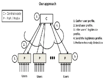
Fig. 4.2 Graphical summary of the methodology
To achieve such a result, we will follow the subsequent steps: at first, each PoP applies the PCA to its subset of users to gather the description of the normal subspace, and sends such description to the central node; the central
47
node than applies an AHC algorithm to identify a subset of users considered free of pollution and computes the legitimate-user profile; eventually, each PoP receives the profile and performs PCA-based anomaly detection within its subset of users.
4.2.1 Probe side: PCA analysis
Given Xp users and the N features we decided to extract
from the CDRs, each probe p performs PCA on the matrix Qp = Xp× N, as shown in section 3.1. At the end
of the process, each probe gather its own PCs, that represent a snapshot of the behaviors of the users they serve, and splits the new reference system into the normal and anomalous subspaces with the cumulative percentage method. As in the centralized approach, the first Lp components able to collect the 95% of the energy
of the dataset are chosen to describe the normal subspace. Eventually, each probe sends to the central node the following information:
the matrix V, which contains all the PCs of the subset, the number of components Lp that describe
48
the ordered eigenvalues of Qp. This type of
information is used to find similarities within the new reference systems obtained by the probes.
the number of users of its own subset Xp, the sum of
the column of Qp, i.e. µp, and its partial Covariance
Matrix CovParp. This information is the same we
used in a previous section to parallelize the computation of the covariance matrix of the whole dataset, and it will be useful in following steps to obtain in the central point the PCs of the dataset we consider free of pollution without any approximation, although the central node does not have the raw data.
4.2.2 Central node side: gathering the
legitimate user profile
The goal of this step is to identify the community of probes, which encloses the description of legitimate users. The supposition made is that probes that do not contain outliers act in the average in the same way and have similar PCs that describe the normal subspace (we will call them PCp) even if they only see different parts
49
similar and discover the “clean” community through an Agglomerative Hierarchical Clustering algorithm. In the following, we refer to such community as CN.
Hierarchical clustering mechanism is proven to work well when coupled with outlier detection techniques[4]. AHC creates a hierarchy of clusters, which may be represented in a tree structure called dendrogram, following a bottom-up approach. The leaves of the tree correspond to each individual probe and the root consists of a single cluster containing all the probes. The algorithm starts from the leaves and successively a series of merging operations follows that eventually forces all the probes into the same cluster. The choice of the clusters to merge is determined by a linkage criterion, which is a function of the pair wise distances between observations: in our case, we use a Weighted Euclidean Distance metric to evaluate how different the PCs of the probes are.
Given M probes, the central node computes the mutual Euclidean distance between the PCp of one probe
towards the PC of the other M-1 probes following these steps:
50
in case the probes have a different number of components describing the normal subspace, the central node computes the distances between the probes considering a number of PCs equal to L =
maxp=1,…M{ Lp }.
considering the PCs mutually orthonormal, the central node computes for each possible couple of probes, only the Euclidean distance of PCs that belong to the same column of matrix V, i.e. it computes dj(PCp,PCq), the distance between the j-th
components of the probes p and the j-th components of the probes q.
due to the fact that the more the energy a PC is able to collect, the more the behavior it is describing is present within the dataset, we decide to give to the first components more importance in the computation of the total distance between the PCp of different
probes. For this reason, the mutual Euclidean distance between two probes is computed as follows:
51
where represent the average percentage of energy the j-th component counts for in the couple of probes we are analyzing on the total energy of their normal subspace. The computation of is made through the following equation:
Given such computation, the maximum Euclidean Distance between probes is .
Once the central node has computed the Euclidean distance between all probes, the AHC algorithm aggregates the pair of probes that exhibit the minimum mutual distance into one cluster. The distance between this new cluster and a given probe is then the average of the distances between the probe and each member of the cluster:
The algorithm iterates joining probes until one of the following two conditions are reached: the mutual Euclidean distance between clusters is over a given
52
threshold S, or all the M probes are grouped into one single cluster.
An example of how a dendrogram can be in our context, considering 20 probes and a given threshold S as stop condition follows in Fig. 4.3.
Fig.4.3 Example of a Dendrogram
In our methodology, the threshold S is set to the average of the minimum Euclidean distances between a given probe towards the other:
53
When AHC returns, the cluster that contains the majority of probes is defined as the community CN, while the
remaining probes belong to the community of outsiders called CA. The supposition behind this decision is that the
outliers, or group of outliers, changes the description of the normal subspace each in a different way and the biggest group that acts in the same way is free of pollution. By the way, we will see in the following section how to avoid taking the wrong community in the case a huge number of outliers of the same species affect the description of the normal subspace of several probes. At this point the central node gathers the description of the legitimate-user profile, by computing the PCs that describe the normal subspace of CN, namely PCN. The
computation is performed starting from the covariance matrix C of the probes belonging to the clean community, based on the information already sent by its probes:
All this information is already present in the central node, and can be gathered with the following computation:
54
.
In this way, the PCN are obtained without sending the
raw data to the central node and without any approximation. From the covariance matrix all the PCs of the clean community are easily computed through the determination of its eigenvectors and eigenvalues. As for the single probe, also in this case the number of PCs representative of the normal subspace is chosen by using the cumulative percentage method and 95% of the total energy of CN as the minimum amount of energy it has to
collect. It is worth noting that this new set of PCs better describe the legitimate user profile with respect to those computed by the single probes, given that it is computed on a more complete set of normal users.
Hence, the central node distributes back to the probes the
PCN, together with the value of the threshold S, the array
GN and the averages . This kind of information is sent
because the probes will use them to perform a cross-check of the profile being gathered.
55
4.2.3 Community check: the Joining Phase
Before performing anomaly detection, each probe checks whether the profile actually corresponds to one of legitimate users. Indeed, it may happen that the AHC algorithm chooses the wrong community, even if this community represents the bigger community within the network. In fact, it is possible that probes with a widespread type of outliers have similar PCs, that they are grouped in the same community and, in a period of time where the number of outliers is not negligible and the CN counts for a small number of probes, which this
type of anomalous community becomes the bigger community within the network. In this case, the particular type of outliers characterizing the subset of probes wrongly chosen as CN will pollute the
computation of PCs and they will go completely undetected in the anomaly detection stage.
To prevent this problem each probe belonging to CA
performs the following scheme:
1. compute the SPE of their own users, normalizing them by the averages of the column of CN, i.e. ,
56
where h is a column vector Xp×1 of 1’s;
2. sort users by their SPE;
3. discard the user with the highest energy accordingly to the legitimate profile received;
4. compute their own PCp without considering
discarded users;
5. if the mutual distance between PCN and PCp,
computed as:
where is the number of PCs of the normal subspace of CN, is bigger than S go to step 2;
6. the probe successfully joined the clean community. In case the central node gathers a polluted profile, i.e. CN
contains widespread anomalies, probes without that kind of anomaly will not obtain PCp that satisfies the
57
condition of Step 5 and an unsuccessful joining phase reveals that.
At the end of this phase the probes communicate to the central node whether they were able to join CN or not. In
case of failure, the central node picks the next-largest community identified by AHC as CN, computes its PCs
and sends them with the additional information mentioned before to the probes. The probes belonging to the new CA repeat the joining phase. If the joining is still
unsuccessful, the central node increases the threshold S by the 10% and repeats the procedure, until all the probes send a positive feedback about the profile PCN. Note that
in case S reaches the maximum d(PCp,PCN), all probes
are grouped into one cluster, and our method becomes equivalent to the centralized approach. In Fig.4.4 we show a case where all the probes erroneously belonging to CA not able to join the “clean” community.
58
Fig.4.4 Wrong CN detection
As we can see from the picture, the Euclidean Distance grows instead of decreasing when we remove the most “anomalous” users, meaning that they are not able to gather the same common behavior of CN.
Thanks to this procedure we are also able to avoid problems when the threshold S is too low and a small number of probes is not able to reach such grade of similarity with CN. In Fig.4.5 there is a case where this
happened, with only two probes not able to reach the low threshold S.
59
Fig.4.5 Unsuccessful joining phase towards the correct CN
In general, if CN is chosen correctly all the probes reach
the same PCs removing a small number of users and the joining phase successful ends, as in the case we show in Fig.4.6.
60
Fig. 4.6 Successful joining phase
4.2.4 Probe Side: Anomaly detection
When the central node receives the successful feedback from all the probes, sends back an acknowledgment to the probes and the anomaly detection stage starts. Note that all the probes can exploit the PCN they already have.
This anomaly detection stage serves the purpose of detecting the users responsible for anomalous behaviors in phone traffic, based on the profile gathered at the central node with the procedure just presented.
During this phase, each probe, even the probes belonging to CN, maps its subset of users onto the PCN, and
61
computes their energy into the anomalous subspace. This operation corresponds to computing the following SPE for each user:
.
The probes then compare the SPE of each user with a threshold value Tp, which is set by each probe by means
of Montecarlo simulations, and label all users with a as anomalous.
62
5
Experimental Results
To apply our methodology to a distributed scenario as described in Chapter 4 from the available data, users that appear in the first day under analysis have been randomly split among a typical number of probes that a telecomm operator can have, i.e. 20 probes. In the following days, the same association user-probe is kept if the user is present the days before, otherwise we randomly assign it to one of the probes. In this way, we end up with approximately 8K users for each probe.
For each day, we compute the matrix Qp of each probe,
and consequently the description of the normal subspace
PCp, by following the procedure outlined in the previous
chapter.
In the first part of this chapter we will show the results of our methodology related to one initial random assignment between users and probes. In the second part of this chapter we will show the comparison of those results to the one obtained from the centralized PCA-based approach. However, experiments were repeated by
63
randomly varying the initial assignments, verifying that the reported considerations hold.
5.1
Numerical evaluation of the Distributed
anomaly detection technique
In this section we propose the numerical results we obtained with the distributed methodology proposed. To avoid showing repetitive results, in this section we only use the most interesting week of the five available ones.
5.1.1 Probe side: PCA analysis
In our simulation, each day the probes present in the network started this phase extracting from the CDRs the features we decide to use regarding incoming and outgoing calls of the users it is in charge of.
To decide to which day a call placed across two different days belongs, we use the lasting timer as assignment parameter. If the interpreters of the call under analysis belong to the telecom operator, the same call is considered both in the computation of the statistics concerning the incoming calls of the callees, and in the computation of the statistics of the outgoing calls of the
64
callers. If only one of the interpreters belongs to the telecomm operator, the call is only used to evaluate the statistics of the internal user. Also evaluating the statistics of the external user can be misleading because we only have partial visibility of their behavior, i.e. their interaction with the internal users of our telecomm operator.
At the end of the feature extraction phase, each probe ends up with its Qp, and following the procedure
illustrated in the previous chapter, computes its own PCp.
To compare how different the local PCs in this initial stage for the week under analysis is, we show Table 5.1.
Day Average Maximum Max #PCs Norm. Subspace Threshold S for AHC Monday 0.258 0.629 4 0.118 Tuesday 0.287 0.622 4 0.139 Wednesday 0.333 0.578 5 0.128 Thursday 0.360 0.559 5 0.129 Friday 0.333 0.585 5 0.143 Saturday 0.382 0.775 5 0.144 Sunday 0.419 0.674 5 0.150
65
As we can see from the table, each day presents at least a couple of probes that gathers PCs for the normal subspace completely different from each other (near the 50% of the maximum possible). In general, this difference is due to a few users present in one of the two probes acting differently from the legitimate behavior, i.e. the behavior shown from the majority of the users, and it is a demonstration of how easily the computation of the PCs can be polluted.
On the other hand, the threshold set from the AHC algorithm for the determination of the clean community is very low if compared to the average distance shown from the probes. For this reason, only probes with a high degree of similarity can be part of CN.
In Fig.5.1 we show the situation of the Weighted Euclidean Distance between the probes in the day of the week where the PCs are in average more distant from each other, i.e. Sunday.
66
Fig. 5.1 Heat map - Initial Condition
In this heat map the distance between probes is shown through colors. The cold colors represent probes with PCs very similar to each other, instead the hot colors represent probe with very different PCs.
Even in this day where the PCs are in average different from a probe to another, the heat map points out interesting patterns. There are clusters of several probes where the mutual distance d(PCp,PCq) is towards zero,
suggesting that those probes have a similar description of the normal subspace. For this reason, they represent a single community during the AHC algorithm since they have users that act in general in the same way. However,
67
some probes differ from all others and result in a yellow stripe in the heat map (e.g. probe number 11). Finally, there are probes which share a similar description of their normal subspace, but such description differs from the behavior described by the majority of the probes: a yellow stripe interleaved by blue square is the visual representation of such pattern. Even though this type of probes does not count for the majority of the probes, they will be a single community too under the AHC algorithm.
5.1.2 Gathering the legitimate profile
Thanks to the methodology, the central node have gathered every day a community where each probes is able to join before the distributed technique becomes equal to the centralized one, i.e. the probes is considered as a single cluster. In Table 5.2 we show the results for the same week presented in the preceding section.
68 Day Maximum Probes ϵ CN Number PCs Norm. Subspace PCN Monday 0.091 9 3 Tuesday 0.080 9 3 Wednesday 0.095 6 4 Thursday 0.136 4 4 Friday 0.065 3 4 Saturday 0.091 8 4 Sunday 0.073 3 4
Tab 5.2 Situation after all probes join CN
As we can see from the table, after the “joining of the community phase” each probe is very close to the PCs gathered from the CN community. This means that in
every day we are able to gather a general description of the behavior of the users that can be found in each probe, i.e. the legitimate profile. If we compare the PCs gathered from each probes to the one gathered from the other probes at the final stage of the procedure we can find a situation as the one in Fig.5.2.
69
Figure 5.2 Final stage gathering legitimate profile The PCs gathered from each probe during the “joining phase” are not only similar to the PCs of the CN, as we
can see also from the last line of the picture where PCN is
reported, but also to each other.
It is also possible to see that in general less than the 50% of the probes belong to the clean community. This means that at least the 50% of the probes gathers a polluted description of the normal subspace in the initial stage, but is able to point out the users responsible for this pollution.
Finally, to collect the 95% of the energy, the clean community needs a smaller number of PCs. Indeed, only
70
considering the users that follow the legitimate profile make easier the description of the normal subspace through the Principal Component Analysis.
But what is the legitimate user profile gathered during this stage? Each day the methodology computes the PCN
based to the behavior of the users it is analyzing, and in general we obtain different snapshots for different days. What is interesting is that the first PCs of the clean community is fundamentally stable in the five weeks, and let us analyze the nature of the legitimate profile.
71
From Table 5.3, the first PC is able to collect more than the 50% of the whole normal subspace. Considering that the PCs are the orthonormal directions composing the new reference system gathered through PCA, the sum of the square weights of each feature is the same if it is done through the 10 PCs, so how much a feature is present in the normal subspace, the more this feature will be well approximated only using this description. For this reason, according to our dataset and the partial representation of the normal subspace shown, we find that legitimate-users can place and establish a number of calls that spans over a wide range and towards a number of callees that can vary, while his number of received calls, their establishment ratio and the number of callers has to be close to the average of the dataset.
This representation of the normal subspace shows that most of the variability of our dataset is due to active features.
72
5.1.3 Anomaly Detection stage
As we said in the preceding chapter, to perform anomaly detection, we order the users by the energy they have in the anomalous subspace after mapping them onto the
PCN and we perform a Montecarlo simulation for each
probe, even for the probes belonging to CN, to set a
threshold Tp to discriminate between legitimate and
anomalous users.
At the end of this stage we inspect the characteristic of the users labeled as anomalous and we discover that most of them act as well-known malicious users or that they are enduring an attack. Remember that we are working in an unsupervised scenario, without any kind of ground truth, except 4 telemarketers confirmed by the telecomm operator.
All the users pointed out in this phase can be profiled in the following eight major behaviors:
users that place almost all the calls where they are involved (at least 90% out of the total), with a low percentage of establishment (at most 30% of the calls placed, but in general under the 10%) and towards a
73
few number of callees (at most the 20% of unique callees on the total number of calls placed). This are statistics that can be found when an attacker is carrying out a DoS attack, i.e. he is repeatedly calling the same user to put out of order its terminal or making him stop answering.
users that place almost all the calls where they are involved in (at least 90% out of the total), with a percentage of establishment near the 50% towards a big number of callees (at least the 75% out of the total number of calls placed). This statistics are similar to the ones belonging to the only ground truth we had, i.e. 4 telemarketers confirmed by the telecomm operator, that our methodology was able to always point out when they were active during the period under analysis.
users that place almost all the calls where they are involved in (at least 90% out of the totals), with a high percentage of establishment (at least 80% of the calls placed) towards few callees (less than 20% if compared to the number of placed calls). This type of behaviors seems to be anomalous but not critical. Due
74
to the fact that those users count for at least 50 to 700 calls placed every day, however this profile shows strong relationship between users.
users with a received out of places call ratio of at least 90%, with a low percentage of establishment (30%) from few callers (less than 10% compared to the number of received calls). This type of profile can appear in the case a user is under a DoS attack, as said before.
users with a received out of places call ratio of at least 90%, with a percentage of establishment less than the 20%, from a big number of callers (at least the 50% compared to the total number of calls received). This type of statistics is the same we can found when a user is under a DDoS attack. Differently from the previous profile, more than one user starts calling the same callees, involving all its available resources.
users with a received out of places call ratio of at least 90% with a high percentage of established call from a big number of callers (respectively at least
75
80% and 60% out of the total calls received).This is a typical behavior a call-center can have.
users with a received out of places call ratio of at least 90%, with a high percentage of establishments (at least 80%) from few callers (less than 10% out of the calls received). Also in this case users are anomalous but probably not malicious.
users with at least 20 calls with network error calls or ending with a suspicious code. This kind of users can represent a problem within the network.
In Table 5.4 we report the number of users for each profile pointed out in the week we are discussing.
Profile # of users DoS victim 40 DDoS victim 11 Call Center 12 Bugged User 55 User Bugger 14 DoS attacker 129 Telemarketer 11 Network problem 63