data-assimilation and spectral nudging
∗ Patricio Clark Di Leoni1, Andrea Mazzino2, & Luca Biferale11Department of Physics and INFN, University of Rome Tor Vergata,
Via della Ricerca Scientifica 1, 00133 Rome, Italy.
2
Department of Civil, Chemical, and Environmental Engineering and INFN, University of Genova, Genova 16145, Italy. (Dated: October 29, 2018)
Inferring physical parameters of turbulent flows by assimilation of data measurements is an open challenge with key applications in meteorology, climate modeling and astrophysics. Up to now, spectral nudging was applied for empirical data-assimilation as a mean to improve deterministic and statistical predictability in the presence of a restricted set of field measurements only. Here, we explore under which conditions a nudging protocol can be used for two novel objectives: to unravel the value of the physical flow parameters and to reconstruct large-scale turbulent properties starting from a sparse set of information in space and in time. First, we apply nudging to quantitatively infer the unknown rotation rate and the shear mechanism for turbulent flows. Second, we show that a suitable spectral nudging is able to reconstruct the energy containing scales in rotating turbulence by using a blind set-up, i.e. without any input about the external forcing mechanisms acting on the flow. Finally, we discuss the broad potentialities of nudging to other key applications for physics-informed data-assimilation in environmental or applied flow configurations.
INTRODUCTION
Extracting information from experimental or observa-tional data of fluid flows is a highly challenging task. While in laboratory experiments one can control and/or measure the properties of the system (e.g. viscosity, ther-mal expansion coefficient, large scale shear, rotation rate etc...), this is often impossible when performing observa-tions in the open field, such as for meteorological data taken from the atmosphere or astrophysical data in the sky. Thus, one has to resort to other methods to infer the desired parameters, a task which most of the time is obstructed by the quality of the data at hand. The problem is part of a vaster paradigm that goes under the name of data assimilation and optimal reconstruction, where one is faced with the need to infer the flow pa-rameters or to extrapolate measurements from a sparse sub-volume of the flow field to the whole space. The problem is also connected to the need to control and improve predictability for the evolution of chaotic sys-tems by using only a partial set of information about the full trajectory. These problems can be encountered in a wide range of fields, going from atmospherics sciences [1, 2], astrophysics [3], optics [4] and medical physics [5]. Several tools have been developed to tackle these chal-lenges. In the context of numerical weather prediction, variational principles and ensemble filters have been de-veloped to fine-tune the parameters entering in the sub-grid models [6–9]. Alternatively, other techniques cou-pled with Bayesian inference, machine learning and deep learning have been proposed to estimate the parameters phase-space in Reynolds-averaged Navier-Stokes models
∗Postprint version of the manuscript published in Phys. Rev.
Fluids 3, 104604 (2018).
in engineering problems [10–13]. Also, information the-ory and statistical mechanics tools such as belief propa-gation have been used to infer parameters from turbulent flows by looking at the motions of transported particles [14]. Another interesting example is the use of sparse regression methods to discover not only parameters but the actual form of the terms controlling the evolution of a system [15, 16].
In this paper, we explore a new avenue and we show how to infer the physical flow parameters from partial data assimilation by exploiting the equations of motion in a dynamical way, using a technique known as nudg-ing, whose conceptual foundation goes well beyond ap-plications to physics (see 2017 Nobel lecture on Econ-omy by R.E. Thaler). Contrary to the attempts previ-ously mentioned where the modeled flow is usually com-pared with data by using a cost function, nudging in-troduces an extra term in the dynamical equation where partial information from field measurements is inputted and exploited to reconstruct the unmeasured degrees-of-freedom. Nudging, has been successfully used and de-veloped to input global circulation model into a regional climate model [17–19]. In this case, due to computa-tional constrains, the global models can not solve the smallest dynamically active scales so as to have accu-rate local weather predictions, while the regional models can not solve for the large planetary cyclonic and anti-cyclonic circulations. Nudging is applied to match the overlapping scales in each model by forcing the regional model to behave as the global one via a penalty term. Outside numerical weather prediction, nudging has also been rigorously applied to estimate bounds in the data assimilation problem in two dimensional Navier-Stokes equations [20, 21], the three dimensional Navier-Stokes α-model [22], and in Rayleigh-Bernard convection [23]. It has also been used to study synchronization in maps and dynamical systems [24]. To the best of our
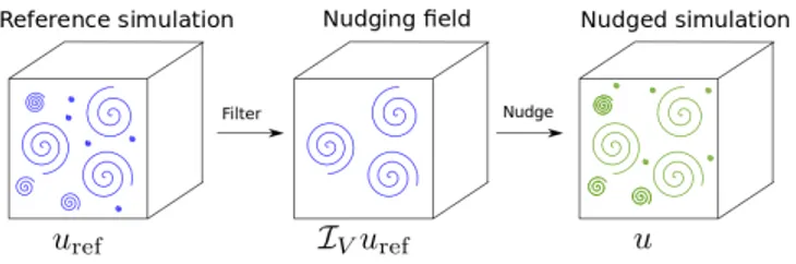
FIG. 1. Diagram showing the set-up of our numerical ex-periments. First, a reference simulation is performed (left). Second, a subset of data is filtered out of the reference field, by keeping only data on a given sub-set of points in space and instant in times (center). Third, we interpolate in time the input partial information and use it to nudge the evolution of a new field to reconstruct the missing data and to infer the correct physics parameters (right).
edge, no attempts have ever been made to benchmark and optimize its performances to the three-dimensional Navier-Stokes equations in the fully developed turbulent regime, characterized by high chaoticity and by a high-dimensional strange attractor.
We implement a spectral nudging technique with two novel aims. First, we show how to use nudging as a physics-informed tool to accurately infer key flow param-eters as, e.g. the rotation rate or the large-scale stirring mechanism, from a limited sub-set of data sparsely mea-sured in time and in Fourier space. Second, we show that the same technique can be used to learn the global physical turbulent configuration. We do this by using the nudged equations to reconstruct in space the large-scale energy distribution of rotating turbulence under the pres-ence of a split energy cascade and without inputting in to the algorithm any information about the external forcing mechanism and about the intensity of the rotation rate. Nudging is thus presented as a general data-driven algo-rithm to learn from sparse measurements in a dynamical way and a with a broad range of applications. Finally, we discuss a series of open challenges to adapt and ex-tend the application of nudging to other turbulent flow configurations using either Eulerian or Lagrangian field measurements and in different domains.
THE NUDGING TECHNIQUE
As said, nudging means to gently convince a numerical flow to evolve as close as possible to a reference set sup-posing to have only partial measurements or observations of the latter [17–19]. The idea is to use the equation of motion to perform an optimal data and flow-parameter assimilation in the interval of time t ∈ (0, t0) and in the whole fluid volume. Suppose we have a reference three dimensional turbulent flow, uref(x, t) evolving
un-der the action of a set of external forces, F [uref, Vref],
parametrised by a set of physical coefficients, Vref =
(Ωref, Sref, `ref, ∆Tref, · · · ) where we denoted with Ωref
the rotation rate, with Sref the amplitude of a large scale
shear with the typical length scale `ref, with ∆Tref the
temperature difference across the volume etc... Suppose that we have access to the measurements of the reference velocity field, uref on a limited set of M anemometers
placed in xj with j = 1, · · · , M that record the flow
properties at N time instants tn with n = 1, · · · , N , i.e.
we control urefin a given sub-domain of the whole
space-time (3+1) volume only. The idea behind nudging is to evolve an independent three dimensional incompressible Navier-Stokes (NS) equations with an initially educated guess for the set of parameters, V, and imposing a pe-nalisation whenever the flow field does not reproduce the inputted velocity values of the reference field in the space-time domain V = (xj, tn):
∂u
∂t+u·∇u = −∇p+ν∇
2u+F [u, V]−αI
V(u−uref) (1)
where ν is the viscosity, p is the pressure that ensures the incompressibility condition, IV is a dimensionless linear
projector operator given by the characteristic function of the set V , and α is a parameter that controls the in-tensity imposed by the nudging control and has units of frequency. In its crudest form, IV is equal to 1 for
(x, t) ∈ V and 0 otherwise. The simplest and most com-mon improvement is to linearly interpolate the different measured snapshots between each time tn and tn+1. So
when entering (1), uref will always be assumed to be
piece-wise differentiable in time with a characteristic in-terpolation window, τ . In this way the operator IV is
only acting on the spatial part of the fields. The whole protocol is sketched in Fig. 1. It is important to real-ize that, in our application, we do not even require to know the exact way the system is forced, i.e. we do not impose V = Vref and the only a priori information that
we provide is inside the partial measurements of the ref-erence field. Clearly, the success of the reconstruction will depend on the amount of information provided (how many measurements in space and in time), on its quality (where and what we measure) and on the intensity of the penalization term, α. Notice that, because of potential stiffness and truncation effects arising when α is big, it is not a priori obvious that taking large α is the best choice. It is intuitive to imagine that in some cases it might be better to allow for a larger error in some mea-suring stations to allow the field to be closer to the target globally.
SET-UP OF THE NUMERICAL SPECTRAL NUDGING EXPERIMENT
We start first by restricting to the case when the set of external parameters are given by the intensity of the Coriolis force due to the presence of a rotation Ω in the vertical direction and of an external stirring mechanism S:
F [u, V] = 2Ω ˆz × u(x, t) + S(x). (2) where S is a randomly-generated, quenched in time, isotropic field with support on wavenumbers with am-plitudes k ∈ [kf 1, kf 2] whose Fourier coefficients are
given by ˆS(k) = Sk−7/2eiθk, where θ
k are the random
phases. In the remaining part of this paper we will ad-dress the most ideal case when the information is supplied in Fourier space, i.e. we imagine to have a periodic array of measurement stations that allow us to reconstruct the reference flow configuration in a given range of nudged wavenumbers, k0< k < k1. In this case, the IV operator
reduces to a band-pass Fourier filter of the form
IVu =
X
k0<|k|<k1
ˆ
u(k, t) exp (ik · x), (3)
that projects the velocity field on the window of nudged Fourier modes.
We implement the whole protocol as follows. First we numerically produce a full space-time evolution of the whole uref field in a interval t ∈ (0, Ttot) by
solv-ing the Navier-Stokes equations with a reference rota-tion rate Ωref and a given intensity of the shear Sref (i.e.,
Eqs (1) with α = 0). The values of Ωref and Sref (and
also ν which is the same for both the reference and the nudged simulations) are given in Table I. All reference simulations are started from rest and allowed to reach stationary states (t = 0 denotes the start of the station-ary states). Second, we extract the inputting field in a subset of discrete times tn = nτ with τ chosen as a
fraction of the characteristic eddy turnover time of the flow (see Table I) . Third, we define the nudging field (3) by a linear interpolation between tn and tn+1 for all
intervals. The initial condition used for all nudged simu-lation is just the first extracted input field (i.e., the field at t = t0) with all the modes outside the nudging
re-gion filtered out. All simulations have been performed with a parallel pseudo-spectral code. The code uses a two step Adams Bashfort scheme for the time integra-tion, the “2/3 rule” for dealiasing and periodic boundary conditions in all three directions. In the following we will analyze three different nudging protocols. The first two cases are about simulations made to infer the physical flow parameters, Ωref and Sref (called INFER1 and
IN-FER2 in the following, see also Table I for details). The third case is about the reconstruction of the large-scale coherent structures and it is called PHYS1. Numerical details for all set-ups can be found in Table I. The value of τ is such that it is smaller than the decorrelation time of the fastest nudged mode, while α was taken as 1/τ , these choices follow common practices [25]. A comprehensive report about the performance of nudging at changing α, τ for fully developed homogeneous and isotropic turbulent flow is not the scope of this paper and it will be presented elsewhere.
Set-up Ekin T ν Re Sref [kf 1, kf 2] Ωref [k0, k1]
INFER1 1.84 3.28 0.002 6030 0.005 [1,2] 2 [1, 4]
INFER2 1.20 4.06 0.0025 4900 0.02 [1,2] 0 [1, 4]
PHYS1 0.0012 128 0.002 150 0.004 [10,11] 20 [8, 20] TABLE I. Parameters used in the different numerical experi-ments. INFER1 is the set-up for the Ω scan, INFER2 for the S scan, and PHYS1 for the inverse cascade experiment. The values listed are the total kinetic energy Ekin= 1/2h|u|2i, the
eddy turnover time T = L/(2Ekin)1/2, with L = 2π being the
largest scale in the flow (same for all simulations), the viscos-ity ν, the Reynolds number Re = L(2Ekin)1/2/ν, the forcing
intensity of the reference simulation Sref, the band of forced
wavenumbers in the reference simulation [kf 1, kf 2], the
rota-tion frequency of the reference simularota-tion Ωref, and the band
of nudged wavenumbers [k0, k1]. The number of grid points
N3
grid = 2563, the time step of the simulations dt = 0.001,
the nudging intensity α = 10, and the temporal interpola-tion window of the nudging field τ = 0.1 are the same for all simulations. The box length L, the temporal timestep dt, the resolution Ngrid3 , and the viscosity ν are the same for the
reference and the nudged simulations in each set. The kinetic energy and Reynolds numbers are given for the reference run of each set, the nudged ones have very similar values.
INFERRING PHYSICAL PARAMETERS IN ROTATING TURBULENCE
We start by asking how to guess the exact value of the rotation rate, Ωref, without any a priori knowledge on its
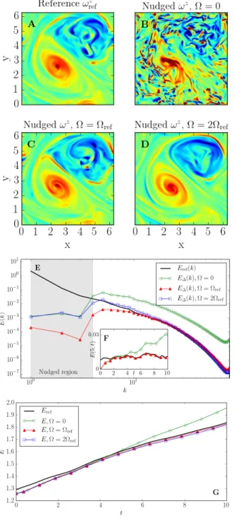
value. To give a first idea on the applications of nudging, in panels (A-D) of Fig. 2 we show a series of 2D slices of the vorticity field in the direction parallel to the rotation axis for the reference simulation (panel A) and for three different nudged simulations (panels B-C-D), two with wrong rotation rates, Ω = 0 and Ω = 2Ωref, and one with
the correct value, Ω = Ωref. Furthermore, in this set of
simulations we took S = 0, i.e. we suppose to not know the forcing mechanism (all simulations are from set-up INFER1 shown in Table I). All snapshots were taken at the same instant in time. Comparing the four panels, it is clear that the simulation nudged with the correct ro-tation rate (panel C) does reconstruct the reference flow (panel A) much better then the other two (panels B and D). It is also worth pointing out that the standard de-viation of the vorticity fields is recovered when rotation is present, with the values begin around 2.8 for the ref-erence and the simulations of both panels C and D, but this is not the case in the absence of ration (panel C), where the standard deviation takes a value around 5.4. All fields have zero mean by construction. These qualita-tive results already provide a first glance of the two main points we make: (i) spectral nudging does work well also for fully turbulent 3D flows, as it does reproduce non-trivial features with high accuracy and (ii) by optimizing the reconstruction properties, one can infer the unknown flow-parameters of the nudging flow. It is worth noticing that the percentage of nudged modes is very small, of the order of #nudged∼ 1 × 10⁻⁴, as we are nudging up to
FIG. 2. Nudging with different rotation rates. Simulations from set-up INFER1 (see Table I). A-D: 2D slices of the vorticity field, ω = ∇ × u, in the direction parallel to the rotation axis for the reference simulation with a rotation fre-quency Ωref, and three nudged simulations performed with
Ω = 0, Ωref, and 2Ωref, respectively. E: Energy spectra of
the reference simulation compared with error spectra E∆(k)
(see Eq. (4)) for different values of the rotation frequency Ω. All spectra were computed at the same instants of time. The shaded gray area indicate the modes where the nudging is acting. F: Time evolution of E(k, t) for k = 5 for Ω = Ωref
and Ω = 0, compared to the reference data. G: Evolution of total energy for the reference field and for the three nudged simulations at changing Ω.
k = 4 while the maximum possible wavenumber in this simulation is k = 85. The nudged modes are the ones containing the largest amount of energy, but the flow is not completely determined by their evolution, as many more scales should be controlled in order to achieve this [26]. This fact is clear when looking at the error spectra in Fig. 2, the error in the unnudged scales is of the order of the energy at that scales even though the large scale re-construction is very good, meaning the unnudged scales are not slaved to the energy containing modes. Some synchronization of the small scales is nonetheless present, specially for the case with Ω = Ωref. Understanding how
much one needs to nudge in order to fully control a tur-bulent flow is an open question that will be addressed in future work.
In order to control the performance of the nudging pro-tocol in quantitative terms and scale by scale, we intro-duce a field given by the difference among the exact input and the one reconstructed via (1), ∆u = u − uref, and
we study its spectral properties: E∆(k, t) = 1 2 X k≤|k|<k+1 | ˆu(k, t) − ˆuref(k, t)|2. (4)
Clearly, the smaller the spectrum E∆(k), the better the
reconstruction. This spectrum will be referred to as the error spectrum.
In the bottom panel (E) of Fig. 2 we show three dif-ferent curves for E∆(k, t) obtained by averaging over
all times when we provide the information, tn, and for
the three different values of the rotation rate, Ω = 0, Ωref, 2Ωref already discussed in panels (A-D), together
with the spectrum of the reference field Eref(k) =
P
k≤|k|<k+1| ˆuref(k, t)|2, averaged on the same set of
times. In the figure, the set of nudged wavenumbers is denoted by the grey area. From panel (E) it is clear that the optimal nudging is obtained when Ω = Ωref is
used in (1), as revealed from the scale-by-scale nudging error, E∆(k), that becomes much smaller than Eref(k)
for k ∈ (k0, k1). In all cases, there is a dip in the error
spectra at k = 3, as this is the first scale at which the forcing is not present in the reference flow, so the nudg-ing is able to do a better job reconstructnudg-ing the data. At k = 4 the error spectra increases again, mainly because some unnudged modes are integrated when calculating the spectra at this wavenumber. For Ω = Ωref, the
scale-by-scale error stays smaller than the reference spectrum up to k ∼ 10 suggesting a good ability for data assimi-lation outside the set of nudged degrees of freedom also. This latter fact is also confirmed by the inset (panel F) where we show the temporal evolution of Eref(k, t) for an
unnudged wavenumber, k = 5, compared with the spec-tra of the reconstructed field evolved with Ω = 0 and Ω = Ωref. In this experiment we started the nudged
sim-ulations from zero velocity. As one can see, after a short transient, only the field evolved with the correct Ω rate is indeed able to synchronize with the time evolution of the inputting data. Finally, we also show the evolution
of the total energy in panel G for the same simulations. While the case with Ω = 0 is easy to pick apart, the other two are very close to tell which is one produces a better reconstruction of the flow. This indicates that compar-ing averaged quantities (such as the total energy) may not be the most precise way to determine the value of a parameter.
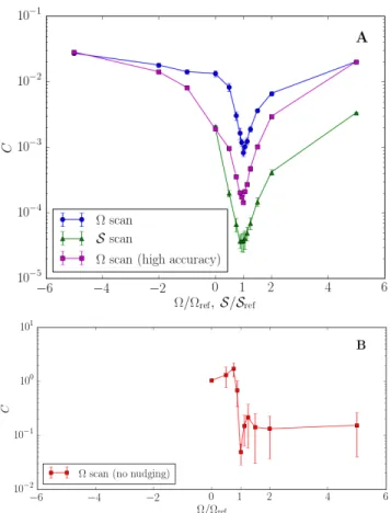
To be more quantitative about the sensitivity to infer the unknown rotation rate, we have performed also a detailed scan of Ω values around Ωref. In Fig. 3A we
show the performance of the nudging reconstruction by plotting the value of the spectrum E∆(k), as a function
of Ω and averaged in time and in the nudged window:
C = 1 N K N X n=1 Z k1 k0 dkE∆(k, tn), (5)
where tn are the instant in times where we have
mea-surements and K =Rk1
k0 dkEref(k) is a normalization
fac-tor. Notice that C is defined using information of the nudging data only, i.e. the filtered reference field at the specific times when the information is provided. In con-trast, E∆(k) needs the whole urefwhich in most practical
applications would not be available, but that we can nev-ertheless access in our numerical experiment.
From Fig. 3A, it is clear the existence of a minimum in the error when evolving (1) with Ω ∼ Ωref. Furthermore,
we can determine the correct value of Ω with a 6.25% error. The error is calculated by looking at which values the errorbars for C overlap. We performed another ex-periment (set-up INFER2 in Table I) to test if the inten-sity S of mechanical forcing of the reference simulation could also be discovered with our nudging protocol. In this experiment a new reference simulation with Ωref= 0
and Sref = 0.02 was produced and used to extract the
nudging fields (see Table I for details). In Fig. 3A we show that the protocol is able to infer the intensity of the stirring mechanism also, with a clear minimum of the error (5) in the proximity of S ∼ Sref. In this case,
the correct value of S can be pinpointed with a 12.5% error. A third experiment, following INFER1 but nudg-ing more wavenumbers (so usnudg-ing more information from the reference as well is shown. Here all wavenumbers up to k = 10 where nudged. By doing this we can reduce the error in the estimation of Ω to 3.125%. All numeri-cal experiments show that spectral nudging can be used in a physics-informed way to fit parameters to data and, thus, extract information from it. Furthermore, in set-up INFER1, where no information about the external stir-ring mechanism is used, performing a one-dimensional scan (i.e. varying only the rotation rate) works well. Having said this, we cannot conclude that this must be the case for generic search in a multi-dimensional phase-space, where the only systematic way to proceed would be to adopt a local gradient-descent algorithm.
A similar scan was performed for the rotation rate but without using the nudging (i.e., α = 0). In this case, the forcing term was also added (with S = Sref), otherwise
FIG. 3. A: Value of the mean error committed to reconstruct the reference field in the nudged window, C, for two different scanning of the phase space parameters. Blue circle: the case with fixed stirring mechanism and at changing the rotation rate Ω (set-up INFER1 in Table I). Green triangles: the case with fixed rotation rate and at changing the intensity of the stirring parameter, S (set-up INFER2 in Table I). Magenta squares: a further scan for Ω following INFER1 but nudging all wavenumbers up to k = 10. In all cases a clear deep is measured only when the scanning values do correspond to the ones used for the reference data, Ωrefand Srefrespectively.
Error bars for each data point were calculated by measuring the standard deviation of C. B: Scan of Ω perfomed without nudging but adding the forcing term (i.e., same as INFER1 but with α = 0 and S = Sref).
there would be no energy injection mechanism present. All other parameters are the same as set-up INFER1. The results are shown in Fig. 3B. It is clear that ob-taining an accurate value of Ω out of this scan is very difficult because even though a minimum is readily seen, the errorbars of several datapoints close to it overlap. So while running simulations with different parameter val-ues and performing posterior analysis in order to infer the desired information is possible, our results suggest the using nudging greatly improves the sensitivity and accuracy of the search.
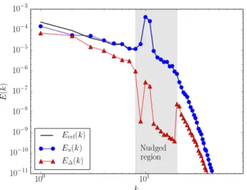
FIG. 4. Nudging for the case of rotating turbulence in the in-verse energy cascade regime. Simulations from set-up PHYS1 (see Table I). The nudged window is given by the grey area between k0 = 8 and k1 = 20. The reference spectrum Eref
and the nudged spectrum Eualmost coincide for k > 8,
mak-ing it hard to discern between the two. Both the intensity of the forcing S and the rotation rate Ω are zero in the nudged simulation, so all energy injection and anisotropic effects are coming from the nudging term. Notice the strongly reduced error spectrum E∆(k) for a large set of wavenumbers,
indi-cating an optimal reconstruction quality.
INFERRING THE LARGE-SCALE VELOCITY DISTRIBUTION WITHOUT INPUT ROTATION
In this section we describe how to use nudging to infer, under some circumstances, the entire set of large-scale physical flow structures of the reference data without a detailed knowledge of the forces acting on flow. To test this idea we performed a new experiment by using a tur-bulent flow under rotation and in the presence of an in-verse energy cascade. It is well known that if rotation is strong enough and energy is injected at large wavenum-bers the flow undergoes a transition from a direct to a split turbulent energy cascade, accumulating kinetic en-ergy and producing a non-trivial cyclonic distribution of vortices at larger and larger scales [27–29]. This regime does not occur naturally in homogeneous isotropic three-dimensional turbulence [30], but it is argued to be impor-tant in many geophysical set-ups in the oceans [31, 32] and in the atmosphere [33]. Here, we show how a suitable nudging strategy is indeed able to reconstruct the inverse energy cascade even in the absence of any explicit rota-tion term in the nudged equarota-tions (1), provided that the uref is inputting information around the injection scale.
To do this we use a rotating turbulent flow forced at kf = 10 and with Ωref = 20 and Sref = 0.004 as a
refer-ence (set-up PHYS1 in Table I) where an inverse energy cascade develops. We then evolve (1) without any
rota-FIG. 5. A: Probability density functions (PDF) of the point-wise kinetic energy for the reference simulation |uref(x)|2
(continuous black line), the nudged simulation |u(x)|2
(cir-cles) and the nudging input field |IVuref(x)|2 (triangles) for
the inverse cascade experiment (set-up PHYS1 in Table I). B-D: 2D slices of planes perpendicular to the rotation axis of the absolute velocity fields.
tion and any external forcing: F [uref, Vref] = 0
in this way we are completely ignorant about the physics we want to reproduce. In Fig. 4 we show that by nudg-ing in the region around the injection mechanism, the energy spectra of the reference simulation is well repro-duced by the nudged simulation even, and in particular, in the inverse energy cascade range. The presence of a strong peak around the forced wavenumber is typical of systems where an inverse cascade is present, as this is a slow and inefficient transfer mechanism [27–29, 34]. Even though the only information we input is the nudging fil-tered field, the nudged evolution is able to reconstruct the inverse cascade and the correct spectrum slope even for scales much smaller then the ones where we nudge. It is remarkable how the spectrum error, E∆(k) is small
also for modes outside the nudging window k < k0 and
k > k1, indicating the presence of strong non-local
spec-tral correlation in the split-energy cascade mechanism which are fully reconstructed by our protocol.
To go beyond spectral properties and to check the abil-ity to reconstruct the large-scale coherent structures in the rotating flow, we plot in Fig. 5 the probability density functions (PDFs) of the space-dependent kinetic energy for the reference simulation, |uref|2/2, the nudged
simu-lation, |u|2/2, and the nudging field, |I
Vuref|2/2. As one
can see, the reconstructed field has a PDF very close to the reference case, even if the nudging input field does not. In the same figure, we also show 2D slices of the absolute velocity fields in planes perpendicular to the ro-tation axis for the three fields as before. As one can
see, the nudged simulation (panel D) is able to extrap-olate the unknown large-scale reference flow structures extremely well (panel B), for a case where the nudged in-putting data do not contain any information about those scale (C). The apparent patterns seen in these visualiza-tions are a product of the strong forcing present in the system acting around k = 10.
CONCLUSIONS
Spectral nudging is a physics-informed technique com-monly used to guide the evolution of chaotic dynami-cal systems inputting measured data. Giving examples for both isotropic and rotating 3D turbulence, we have shown how this technique can be efficiently used to in-fer both the physical parameters entering in the external stirring forces and the large-scale velocity distribution for the inverse energy cascade regime, typical of strongly rotating turbulent flows. The method can be further im-proved and optimised by using different nudging param-eters for different degrees of freedoms, e.g. by changing α and τ with k. A detailed study of nudging perfor-mances for homogeneous and isotropic turbulence at dif-ferent Reynolds numbers, difdif-ferent nudging windows and at changing the spatial locations of the measurements stations will be reported elsewhere.
Other strategies used to estimate parameters, such as variational methods [35] or ensemble based methods [7– 9], require the need to postulate and error correlation matrix and make assumptions about the behavior of the errors and deviations, need to use linearized models (for variational methods), or are based on minimizing compli-cated functions (again for variational methods). Nudging based strategies do require to perform several forwards
simulations, similar to ensemble based method. One ad-vantage other methods have compared to nudging, is the ease to incorporate information on observables (such as precipitation, for example) and not just state variables (such as the velocity field, as was used here. Interestingly, variational data assimilation schemes have been exploited to determine vectors of optimal nudging coefficients [36]. Here, we reversed the point of view: given the coefficients α, τ , we employed nudging to estimate the physical flow parameters. Finally, the method is also general and ex-tendable to other problems, opening the route to applica-tions for parameter inferring to a vast set of hydrodynam-ical situations including, to cite just the most promis-ing cases, i) optimispromis-ing sub-grid-scale models in Large Eddy Simulations, by inferring parameters against data extracted from either observation or benchmark direct numerical simulations; ii) large-scale turbulent transport to determine eddy-viscosity and eddy-diffusivity [37, 38]; iii) the identification of ambient air sources and the quan-tification of their contribution to pollution levels (the so-called source apportionment problem) [39]; iv) partial field reconstruction using advanced Lidar systems [40] to reveal the free parameters characterizing the atmospheric boundary layer; v) correction of velocity fields in ocean circulation models with Lagrangian data (e.g. from drift-ing buoys) [41, 42] and/or other sources includdrift-ing HF radar data [43].
ACKNOWLEDGMENTS
The authors acknowledge funding from the Euro-pean Research Council under the EuroEuro-pean Community’s Seventh Framework Program, ERC Grant Agreement No. 339032.
[1] I. F. Akyildiz, W. Su, Y. Sankarasubramaniam, and E. Cayirci, “Wireless sensor networks: a survey,” Com-puter Networks 38, 393–422 (2002).
[2] Jane K. Hart and Kirk Martinez, “Environmental sen-sor networks: A revolution in the earth system science?” Earth-Science Reviews 78, 177–191 (2017).
[3] H. S. Fu, A. Vaivads, Y. V. Khotyaintsev, V. Olshevsky, M. Andr, J. B. Cao, S. Y. Huang, A. Retin, and G. Lapenta, “How to find magnetic nulls and reconstruct field topology with MMS data?” Journal of Geophysical Research: Space Physics 120, 2015JA021082 (2015). [4] P. Carpeggiani, M. Reduzzi, A. Comby, H. Ahmadi,
S. Khn, F. Calegari, M. Nisoli, F. Frassetto, L. Poletto, D. Hoff, J. Ullrich, C. D. Schrter, R. Moshammer, G. G. Paulus, and G. Sansone, “Vectorial optical field recon-struction by attosecond spatial interferometry,” Nature Photonics 11, 383–389 (2017).
[5] Julia Busch, Daniel Giese, Lukas Wissmann, and Sebas-tian Kozerke, “Reconstruction of divergence-free velocity fields from cine 3d phase-contrast flow measurements,” Magnetic Resonance in Medicine 69, 200–210 (2013).
[6] Eugenia Kalnay, Atmospheric Modeling, Data Assimi-lation and Predictability (Cambridge University Press, 2003) google-Books-ID: zx BakP2I5gC.
[7] Jeffrey L. Anderson and Stephen L. Anderson, “A Monte Carlo Implementation of the Nonlinear Filtering Prob-lem to Produce Ensemble Assimilations and Forecasts,” Monthly Weather Review 127, 2741–2758 (1999). [8] Jeffrey L. Anderson, “An Ensemble Adjustment Kalman
Filter for Data Assimilation,” Monthly Weather Review 129, 2884–2903 (2001).
[9] Juan Jose Ruiz, Manuel Pulido, and Takemasa Miyoshi, “Estimating Model Parameters with Ensemble-Based Data Assimilation: A Review,” Journal of the Meteo-rological Society of Japan. Ser. II 91, 79–99 (2013). [10] Marc C. Kennedy and Anthony O’Hagan, “Bayesian
cal-ibration of computer models,” Journal of the Royal Sta-tistical Society: Series B (StaSta-tistical Methodology) 63, 425–464 (2001).
[11] H. Xiao, J. L. Wu, J. X. Wang, R. Sun, and C. J. Roy, “Quantifying and reducing model-form uncertain-ties in Reynolds-averaged NavierStokes simulations: A
data-driven, physics-informed Bayesian approach,” Jour-nal of ComputatioJour-nal Physics 324, 115–136 (2016). [12] Eric J. Parish and Karthik Duraisamy, “A paradigm for
data-driven predictive modeling using field inversion and machine learning,” Journal of Computational Physics 305, 758–774 (2016).
[13] Julia Ling, Andrew Kurzawski, and Jeremy Temple-ton, “Reynolds averaged turbulence modelling using deep neural networks with embedded invariance,” J. Fluid Mech. 807, 155–166 (2016).
[14] M. Chertkov, L. Kroc, F. Krzakala, M. Vergassola, and L. Zdeborov, “Inference in particle tracking experiments by passing messages between images,” Proceedings of the National Academy of Sciences 107, 7663–7668 (2010). [15] Steven L. Brunton, Joshua L. Proctor, and J. Nathan
Kutz, “Discovering governing equations from data by sparse identification of nonlinear dynamical systems,” Proceedings of the National Academy of Sciences 113, 3932–3937 (2016).
[16] Samuel H. Rudy, Steven L. Brunton, Joshua L. Proc-tor, and J. Nathan Kutz, “Data-driven discovery of par-tial differenpar-tial equations,” Science Advances 3, e1602614 (2017).
[17] Kim M. Waldron, Jan Paegle, and John D. Horel, “Sen-sitivity of a Spectrally Filtered and Nudged Limited-Area Model to Outer Model Options,” Monthly Weather Re-view 124, 529–547 (1996).
[18] Hans von Storch, Heike Langenberg, and Frauke Feser, “A Spectral Nudging Technique for Dynamical Down-scaling Purposes,” Monthly Weather Review 128, 3664– 3673 (2000).
[19] Gonzalo Miguez-Macho, Georgiy L. Stenchikov, and Alan Robock, “Spectral nudging to eliminate the effects of domain position and geometry in regional climate model simulations,” Journal of Geophysical Research: Atmospheres 109, D13104 (2004).
[20] Aseel Farhat, Evelyn Lunasin, and Edriss S. Titi, “Abridged Continuous Data Assimilation for the 2d NavierStokes Equations Utilizing Measurements of Only One Component of the Velocity Field,” Journal of Math-ematical Fluid Mechanics 18, 1–23 (2016).
[21] Masakazu Gesho, Eric Olson, and Edriss S. Titi, “A Computational Study of a Data Assimilation Al-gorithm for the Two-dimensional Navier-Stokes Equa-tions,” Communications in Computational Physics 19, 1094–1110 (2016).
[22] Dbora A. F. Albanez, Nussenzveig Lopes, Helena J, and Edriss S. Titi, “Continuous data assimilation for the three-dimensional NavierStokes-α model,” Asymp-totic Analysis 97, 139–164 (2016).
[23] Aseel Farhat, Hans Johnston, Michael S. Jolly, and Edriss S. Titi, “Assimilation of nearly turbu-lent Rayleigh-B\’enard flow through vorticity or lo-cal circulation measurements: a computational study,” arXiv:1709.02417 [physics] (2017), arXiv: 1709.02417. [24] Diego Paz, Juan M. Lpez, Rafael Gallego, and Miguel A.
Rodrguez, “Synchronizing spatio-temporal chaos with imperfect models: A stochastic surface growth picture,” Chaos: An Interdisciplinary Journal of Nonlinear Science 24, 043115 (2014).
[25] Hiba Omrani, Philippe Drobinski, and Thomas Dubos, “Spectral nudging in regional climate modelling: how strongly should we nudge?” Quarterly Journal of the Royal Meteorological Society 138, 1808–1813 (2012).
[26] Cristian C. Lalescu, Charles Meneveau, and Gregory L. Eyink, “Synchronization of chaos in fully developed tur-bulence,” Physical Review Letters 110, 084102 (2013). [27] Leslie M. Smith, Jeffrey R. Chasnov, and Fabian Waleffe,
“Crossover from two- to three-dimensional turbulence,” Phys. Rev. Lett. 77, 2467–2470 (1996).
[28] P. D. Mininni and A. Pouquet, “Helicity cascades in ro-tating turbulence,” Phys. Rev. E 79, 026304 (2009). [29] P. D. Mininni, A. Alexakis, and A. Pouquet, “Scale
in-teractions and scaling laws in rotating flows at moderate rossby numbers and large reynolds numbers,” Phys. Flu-ids 21, 015108 (2009).
[30] L. Biferale, S. Musacchio, and F. Toschi, “Split en-ergyhelicity cascades in three-dimensional homogeneous and isotropic turbulence,” J. Fluid Mech. 730, 309–327 (2013).
[31] Robert B. Scott and Faming Wang, “Direct evidence of an oceanic inverse kinetic energy cascade from satellite altimetry,” Journal of Physical Oceanography 35, 1650– 1666 (2005).
[32] Raffaele Corrado, Guglielmo Lacorata, Luigi Palatella, Rosalia Santoleri, and Enrico Zambianchi, “General characteristics of relative dispersion in the ocean,” Sci-entific Reports 7, 46291 (2017).
[33] Guglielmo Lacorata, Erik Aurell, Bernard Legras, and Angelo Vulpiani, “Evidence for a k−5/3 spectrum from the eole lagrangian balloons in the low stratosphere,” Journal of the Atmospheric Sciences 61, 2936–2942 (2004).
[34] L. Biferale, F. Bonaccorso, I.M. Mazzitelli, M.A.T. van Hinsberg, A.S. Lanotte, S. Musacchio, P. Perlekar, and F. Toschi, “Coherent structures and extreme events in rotating multiphase turbulent flows,” Physical Review X 6, 041036 (2016).
[35] I. M. Navon, “Practical and theoretical aspects of ad-joint parameter estimation and identifiability in mete-orology and oceanography,” Dynamics of Atmospheres and Oceans 27, 55–79 (1998).
[36] X. Zou, I. M. Navon, and F. X. Ledimet, “An optimal nudging data assimilation scheme using parameter esti-mation,” Quarterly Journal of the Royal Meteorological Society 118, 1163–1186 (1992).
[37] Lisan Yu and James J. O’Brien, “Variational estimation of the wind stress drag coefficient and the oceanic eddy viscosity profile,” Journal of Physical Oceanography 21, 709–719 (1991).
[38] Ching-Long Lin, Tianfeng Chai, and Juanzhen Sun, “Retrieval of flow structures in a convective boundary layer using an adjoint model: Identical twin experi-ments,” Journal of the Atmospheric Sciences 58, 1767– 1783 (2001).
[39] M. C. Bove, P. Brotto, F. Cassola, E. Cuccia, D. Massab, A. Mazzino, A. Piazzalunga, and P. Prati, “An in-tegrated PM2.5 source apportionment study: Positive matrix factorisation vs. the chemical transport model CAMx,” Atmospheric Environment 94, 274–286 (2014). [40] D. I. Cooper, W. E. Eichinger, R. E. Ecke, J. C. Y. Kao, J. M. Reisner, and L. L. Tellier, “Initial investigations of microscale cellular convection in an equatorial marine atmospheric boundary layer revealed by lidar,” Geophys-ical Research Letters 24, 45–48 (1997).
[41] Vincent Taillandier, Annalisa Griffa, and Anne Mol-card, “A variational approach for the reconstruction of
re-gional scale eulerian velocity fields from lagrangian data,” Ocean Modelling 13, 1–24 (2006).
[42] V. Taillandier, A. Griffa, P.-M. Poulain, and K. Branger, “Assimilation of argo float positions in the north west-ern mediterranean sea and impact on ocean circulation simulations,” Geophysical Research Letters 33, L11604 (2006).
[43] Maristella Berta, Lucio Bellomo, Marcello G. Magaldi, Annalisa Griffa, Anne Molcard, Julien Marmain, Mireno Borghini, and Vincent Taillandier, “Estimating La-grangian transport blending drifters with HF radar data and models: Results from the TOSCA experiment in the ligurian current (north western mediterranean sea),” Progress in Oceanography 128, 15–29 (2014).