A class of evolutionary models for participation games
with negative feedback
∗
Pietro Dindo
†and Jan Tuinstra
‡July 31, 2010
Abstract
We introduce a framework to analyze the interaction of boundedly rational heteroge-neous agents repeatedly playing a participation game with negative feedback. We assume that agents use different behavioral rules prescribing how to play the game conditionally on the outcome of previous rounds. We update the fraction of the population using each rule by means of a general class of evolutionary dynamics based on imitation, which contains both replicator and logit dynamics. Our model is analyzed by a combination of formal analysis and numerical simulations and is able to replicate results from the exper-imental and computational literature on these types of games. In particular, irrespective of the specific evolutionary dynamics and of the exact behavioral rules used, the dynam-ics of the aggregate participation rate is consistent with the symmetric mixed strategy Nash equilibrium, whereas individual behavior clearly departs from it. Moreover, as the number of players or speed of adjustment increase the evolutionary dynamics typically becomes unstable and leads to endogenous fluctuations around the steady state. These fluctuations are robust with respect to behavioral rules that try to exploit them.
Keywords: Participation games; Heterogeneous behavioral rules; Revision protocol;
Replicator Dynamics; Logit Dynamics; Nonlinear dynamics.
JEL Classification: C72; C73.
1
Introduction
Many economic decisions, such as firms choosing whether or not to enter a new market or to invest in a new technology, commuters choosing a route to the workplace, or suppliers choosing between two locations to sell their products, can be characterized as participation
games with negative feedback. This type of game is encountered whenever a, possibly large,
group of agents is competing for a scarce resource, in the absence of a market institution that acts as a coordination device. Their strategic setting can be exemplified as choosing whether or not to participate in a certain ‘project’, given that the payoff associated with participating ∗Previous versions of this paper have circulated under the title “A behavioral model for participation games
with negative feedback”.
†Corresponding author. LEM, Scuola Superiore Sant’Anna, Piazza Martiri della Libert`a 33, 56127 Pisa,
Italy. E-mail: [email protected]. Phone: +39-050-883591. Fax: +39-050-883344.
‡Department of Quantitative Economics and CeNDEF, Faculty of Economics and Business, University of
decreases with the number of other players taking the same decision. In the terminology
of Haltiwanger and Waldman (1985), actions in negative feedback participation games are
strategic substitutes.1
In this paper we study the interaction of a group of boundedly rational heterogeneous agents who are repeatedly playing a participation game with negative feedback. Drawing from the experimental and computational literature we build a model where agents decide whether to participate or not, using behavioral rules that condition on the outcome of previous rounds, as in Arthur (1994) and Selten et al. (2007). Moreover, through an evolutionary process, more successful rules “attract” a larger share of the population. Such an evolutionary competition between different, possibly sophisticated, behavioral rules, has been successfully introduced in a number of economic environments, such as cobweb models, financial markets, Cournot oligopoly models, and labor markets (see e.g. Brock and Hommes, 1997, 1998, Chiarella and He, 2002, Droste et al., 2002, Neugart and Tuinstra, 2003, and Brianzoni et al., 2010) but is new to participation games.
The existing experimental literature on participation games suggests that when agents play them repeatedly the dynamics of the aggregate outcome is inherently unstable and the par-ticipation rate exhibits persistent fluctuations. At the aggregate level, the first moment of the empirical distribution of participation rates seems to be consistent with the symmetric mixed strategy Nash equilibrium of the underlying one-shot game. Nevertheless, individual subjects do not play according to this strategy. Participation rate fluctuations therefore cannot be eas-ily attributed to the randomization implied by the mixed strategy Nash equilibrium. Subjects seem to base their decisions on different behavioral rules or heuristics. Existing models that have tried to replicate this feature suffer from two drawbacks: they are typically purely com-putational, and they rely on the choice of specific behavioral rules and/or updating dynamics so that the generality of the findings is questionable.
The aim of the present paper is to put forward a simple framework able to replicate the main stylized facts emerging from the experimental and computational results using a general class of evolutionary updating mechanisms and a general class of behavioral rules. Following recent work by Hofbauer and Sandholm (2009), the class of updating mechanisms is characterized by a number of properties of agents’ propensities to switch between rules. It contains some well-known evolutionary models, such as the replicator dynamics and the logit dynamics. The class of behavioral rules is characterized by two stylized properties: agents condition their choices on past participation rates, and agents do not randomize.
We investigate under which conditions such an evolutionary dynamics converges, and if so, whether it converges to a Nash equilibrium of the participation game. In its most stylized form, when only simple behavioral rules are used, our model is low dimensional and analytically tractable. Both properties are lost, however, when more complicated rules are available, but insight into the evolutionary dynamics may then be gathered from numerical simulations. Our first finding is that the participation rate may be unstable and fluctuates around the symmetric mixed strategy Nash equilibrium, even if individual behavior clearly departs from it. This finding is consistent with earlier results from the experimental and computational literature. Secondly, we show that the introduction of new rules that try to exploit a regularity in the time series of participation rates does not stabilize participation. In fact, adding new rules make the resulting time series more irregular and more unpredictable. The endogenous
1In contrast, public good provision, union membership, or technology adoption may be characterized as
participation games with positive feedback, that is, games where the payoff for participating increases with the number of participating players. Actions are in this case strategic complements. See Anderson and Engers (2007) for a similar definition of participation games.
fluctuations found in this type of framework are therefore quite robust.
The remainder of the paper is organized as follows. In Section 2 the one-shot negative feedback participation game is introduced and its Nash-equilibria are characterized. We also briefly discuss the experimental and computational literature on participation games in that section. Section 3 introduces a framework for studying evolutionary competition between different rules and in Section 4 we apply this to a stylized, but very instructive and analytically tractable, example. In Section 5 we use simulations to investigate how the overall dynamics changes when more complex rules are added and, in particular, whether new rules can exploit the emerging patterns of past participation rates. Section 6 concludes. The appendix contains proofs of the main results.
2
The negative feedback participation game
We consider a participation game with N players. Each player chooses an action a ∈ {0, 1}, where a = 1 represents ‘participating’ and a = 0 represents ‘not participating’. The action
space is given by A = {0, 1}N and an action profile by a ∈A. By a−i = (a1, . . . , ai−1, ai+1, . . . , aN)
we denote the set of actions played by all players but player i. The payoff πi(ai, a−i; Nc, N ) is
given as: πi(0, a−i; Nc, N ) = α, πi(1, a−i; Nc, N ) = α + β − γ α − γ if PNj=1,j6=iaj < Nc if PNj=1,j6=iaj ≥ Nc , (1)
where the parameter Nc denotes the capacity of the project. Participating gives payoff α − γ
if Ncor more of the other N − 1 players participate, and payoff α + β − γ if less than Ncof the
other N − 1 players participate.2 We assume α > γ to ensure that payoffs are always strictly
positive and β > γ to ensure that a = 1 is not a dominated strategy. The payoff α corresponds
to some outside payment,3 γ to the cost or effort of participation and β to the return of a
successful project. Note that this is indeed a negative feedback participation game, since an increase in the number of players participating in the project might decrease profitability of the project.
In many experiments on participation games with negative feedback, e.g. market entry games, the payoff for participating is linearly decreasing in the number of other entrants. The present formulation, using a step function for the participating payoff, follows the payoff function for the El Farol bar game that was used in Arthur (1994), Bell (2001) and Franke (2003). We chose this stylized version of the game since it facilitates analyzing the effect of N on the dynamics, while keeping the total number of parameters to a minimum.
A (mixed or pure) strategy si for player i is the probability with which he\she chooses action
a = 1. The strategy space is therefore given by S = [0, 1]N, s ∈ S denotes a strategy profile
and s−i denotes the set of strategies for all players, except player i. Using (1) the expected
2Note that for N = 2 and N
c= 1, this payoff structure is similar to the well-known Hawk-Dove game (see
e.g. Fudenberg and Tirole, 1991, pp. 18-19)
3In this formulation of the game, the payoff α could be set to zero without changing the results. Nevertheless,
since in the dynamic approach of the following sections α does play an important role, we have decided to introduce it at this earlier stage.
payoff of playing strategy si is given by
πi(si, s−i; Nc, N ) = (1 − si) α + si(α + β Pr {N−i ≤ Nc− 1} − γ)
= α + si(β Pr {N−i ≤ Nc− 1} − γ) (2)
where Pr {N−i ≤ Nc− 1} is the probability that the number of other agents participating, N−i,
which is a random variable, is strictly smaller than Nc. Obviously, this probability depends
upon the strategy profile s−i.
2.1
Nash equilibria
Assume that all players are risk neutral and want to maximize their expected payoffs. The game has many pure strategy Nash equilibria (henceforth PSNE). Any strategy profile s such
that exactly Nc players participate with certainty (s = 1) and the other N − Nc participants
abstain with certainty (s = 0) corresponds to a strict PSNE. Evidently, there are¡NN
c ¢
of these
PSNE. Note that such a PSNE leads to an uneven distribution of payoffs, with exactly Nc
players obtaining α + β − γ and the other N − Nc players receiving α. Now consider mixed
strategy Nash equilibria (henceforth MSNE), where some players randomize between the two possible actions. We will prove that there exists a unique symmetric mixed strategy Nash
equilibrium s∗ ∈ (0, 1). If each player participates with probability s∗, the probability that
strictly less than Nc out of N − 1 players participate is given by:
p (s∗; Nc, N ) = NXc−1 k=0 µ N − 1 k ¶ (s∗)k(1 − s∗)N −1−k. (3) Note that p (s∗; N
c, N ) is a polynomial of degree N − 1 in s∗. In particular, p (s∗; Nc, N )
is the cumulative distribution function evaluated at Nc− 1 of a binomial distribution with
N − 1 degrees of freedom and probability s∗. For a mixed strategy Nash equilibrium, s∗ is a
best response for player i only if, given that every other player uses strategy s∗, player i is
indifferent between participating and not participating. That is, at s∗ we must have
πi(1, s∗; Nc, N ) = πi(0, s∗; Nc, N ) ,
which gives
α + (βp (s∗; N
c, N ) − γ) = α. (4)
Hence the equilibrium value of s∗ is implicitly given as the solution of (4), which can be
rewritten as:
p (s∗; N
c, N ) =
γ
β. (5)
The following proposition summarizes the properties of the symmetric MSNE, establishes
uniqueness, and gives the relationship between s∗ and the threshold ratio b ≡ Nc
N.
Proposition 1 For any N, Nc< N , α, γ, β > γ, there exists a unique symmetric MSNE s∗
of the N-player participation game with payoff function (1). The value of s∗ solves (5) and
does not depend upon α. Moreover, s∗ → b as N → ∞ for all γ and β, and s∗ = 1/2 for all
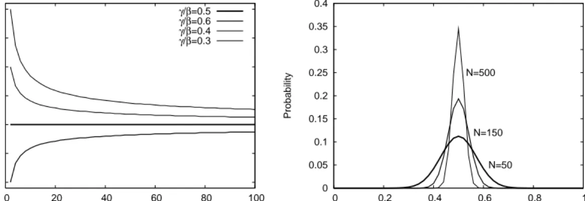
The exact value of s∗ depends on the threshold value b and on the ratio γ/β. Generically it is
unequal to b, but it approaches b as the number of players becomes large. This is illustrated
in the left panel of Fig. 1 which shows s∗ as a function of N for b = 1
2 and different values
of γ/β. Furthermore s∗ = 1
2 for all N when b =
1
2 and β = 2γ, that is when the payoff α is
exactly in between the payoffs of a successful and a non-successful participation.
Note that, when the game is played repeatedly and agents play the symmetric MSNE, the
total number of participating players at time t, Nt, has mean Ns∗ and variance Ns∗(1 − s∗).
The participation rate sequence {xt}, with xt = NNt, would therefore be randomly distributed
around s∗ with variance s∗(1−s∗)
N and with zero autocorrelations at all lags. Observe that as N
becomes large, the distribution of x will converge in probability to a point mass at s∗ as also
illustrated in the right panel of Fig. 1.
0.4 0.45 0.5 0.55 0.6 0.65 0.7 0 20 40 60 80 100 Participation probability Game size N γ/β=0.5 γ/β=0.6 γ/β=0.4 γ/β=0.3 0 0.05 0.1 0.15 0.2 0.25 0.3 0.35 0.4 0 0.2 0.4 0.6 0.8 1 Probability Fraction of participants N=500 N=150 N=50
Figure 1: Symmetric mixed strategy Nash equilibrium. Left panel: Every curve
shows the MSNE s∗, for N up to 100 and b = Nc
N = 12. Each curve corresponds to a different
value of γ/β. Right panel: The distribution of participation rates for three values of N and
equal bins of length 0.02. Other parameters are b = Nc
N = 1 2 and γ β = 1 2.
Summarizing, the PSNE has the characteristic that it extracts all rents from the game, but distributes them asymmetrically over the players, whereas the symmetric MSNE gives the
same expected payoff to each of the players, but may lead to allocative inefficiencies.4,5
2.2
Experimental results on participation games
The experimental literature on participation games with negative feedback has dealt with different realizations of this type of strategic interaction. Market entry games, where payoffs for entering a market are linearly decreasing in the number of entrants, have been extensively analyzed in, among others, Sundali et al. (1995), Erev and Rapoport (1998), Rapoport et al. (1998), Zwick and Rapoport (2002) and Duffy and Hopkins (2005). Iida et al. (1992) and Selten et al. (2007) report on laboratory experiments where subjects have to choose between two roads. Meyer et al. (1992) consider suppliers who have to choose between two locations to sell their product and Bottazzi and Devetag (2003, 2007) present experimental results
4The symmetric MSNE is also the unique evolutionary stable strategy (see Dindo, 2007).
5Asymmetric MSNE, with players randomizing with different probabilities, also exist, for example, with
M < Nc agents always participating and the other N − M agents randomizing with equal probability. In fact, in this case the players randomizing are playing the symmetric MSNE of the participation game with payoff structure (1) but with size N − M and capacity Nc− M .
on the minority game.6 Despite having considered different specifications of participation
games with negative feedback, these experimental contributions have put forward the same findings. Aggregate behavior is roughly consistent with the symmetric mixed strategy Nash equilibrium of the underlying one-shot game, with participation rates fluctuating around the optimal capacity of the project. At the individual level, however, subjects typically do not adhere to the mixed strategy Nash equilibrium. Bottazzi and Devetag (2007) and Selten
et al. (2007), for example, reject the null hypothesis that subjects subsequent choices are
independent. In general, individual strategies are heterogeneous, with some subjects always participating, others never participating and many subjects conditioning their behavior on the outcome in previous rounds.
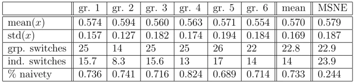
The following experiment on a negative feedback participation game, which we take from Chapter 4 of Heemeijer (2009), nicely illustrates these findings. The experiment involved 6 groups of 7 players, which had to make a participation decision for 50 subsequent periods. The participation game they played could be characterized as α = 100, β = 50 and γ = 25, with
N = 7 and capacity set to Nc = 4. Moreover, a stochastic term ε from a symmetric triangular
distribution on [−25, 25] was added to the payoff for participating in every period. Group composition remained the same over the course of the experiment. At a PSNE exactly four players participate with certainty and the other three do not. The unique symmetric MSNE
is given as s∗ ≈ 0.5786, which is slightly larger than the threshold fraction b = 4
7 ≈ 0.5714. gr. 1 gr. 2 gr. 3 gr. 4 gr. 5 gr. 6 mean MSNE mean(x) 0.574 0.594 0.560 0.563 0.571 0.554 0.570 0.579 std(x) 0.157 0.127 0.182 0.174 0.194 0.184 0.169 0.187 grp. switches 25 14 25 25 26 22 22.8 22.9 ind. switches 15.7 8.3 15.6 13 17 14 14 23.9 % naivety 0.736 0.741 0.716 0.824 0.689 0.714 0.733 0.244
Table 1: Experimental results. The first and second row give, respectively, the average participation rate and its standard deviation for each group. The third row gives the number of times, per group, that participation changed from four or less to five or more subjects or vice versa. The fourth row gives, per group, the number of individual switches between participating and not participating, averaged over subjects. The last row gives the percentage of individual switches that follow directly after a negative payoff experience. The last column gives the corresponding quantities for the symmetric MSNE.
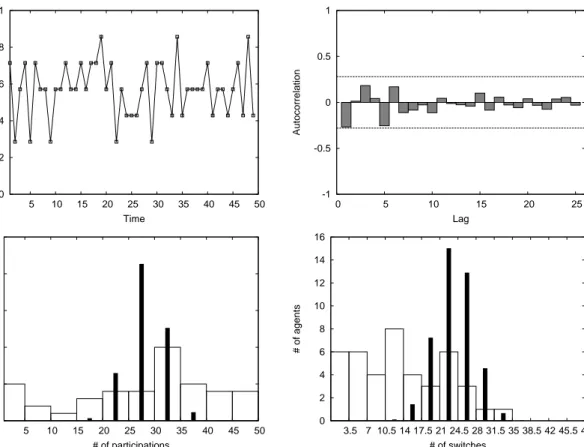
Results from this experiment, which was conducted in 2006 at the experimental economics laboratory of the University of Amsterdam, provide an example of the experimental evidence discussed above. The upper left panel of Fig. 2 shows, for the first experimental group, the dynamics of the number of participating subjects over 50 periods. Behavior in the other groups was similar. Aggregate participation decisions are unstable and keep on fluctuating until the end of the experiment. Fluctuations are quite irregular and the upper right panel shows that no significant linear autocorrelation structure can be detected in the participation rate of group 1. Subjects did not coordinate on one of the PSNE and, at the aggregate level,
6This game, introduced by physicists (see e.g. Challet and Zhang, 1997, 1998, or
http://www.unifr.ch/econophysics), has an odd number of players and positive payoffs only for the players making the minority choice.
0 0.2 0.4 0.6 0.8 1 5 10 15 20 25 30 35 40 45 50 Participants Time -1 -0.5 0 0.5 1 0 5 10 15 20 25 Autocorrelation Lag 0 5 10 15 20 25 5 10 15 20 25 30 35 40 45 50 # of agents # of participations 0 2 4 6 8 10 12 14 16 3.5 7 10.5 14 17.5 21 24.5 28 31.5 35 38.5 42 45.5 49 # of agents # of switches
Figure 2: Upper left panel: Time series of number of participating players in experimen-tal group 1. Upper right panel: Autocorrelation plot for group 1. Lower left panel: Histogram of the number of participations for all 42 participants. Lower right panel: His-togram of the number of switches. In both lower panels the vertical thick lines represent the histogram of participations and switches, respectively, implied by the symmetric MSNE. the symmetric MSNE seems to provide a better description of the data. Note that this is
achieved even if agents cannot compute the value of s∗ as, due to the stochastic term ε, they
do not know the exact value of the payoffs. The first row of Table 1 shows that average
participation rates in all groups are quite close to s∗ ≈ 0.5786.
At the individual level, however, the symmetric MSNE is not supported by the data. The lower left panel of Fig. 2, for example, shows a histogram of the number of times the 42 subjects participated. Apparently, some subjects participate almost always, whereas others participate almost never. Further evidence is given by the third and fourth row of Table 1, which show that, although the number of switches in aggregate participation are roughly consistent with the symmetric MSNE, individual subjects change their participation decision much less frequently. The histogram of the number of individual switches, depicted in the lower right panel of Fig. 2 also provides compelling evidence that many subjects are quite reluctant to change. In both histograms of Fig. 2 the differences between the empirical distribution
and the distribution where players use s∗ are striking. Instead of playing according to the
symmetric MNSE, subjects seem to condition their decision on past payoffs. The last row of Table 1 shows that about 73% of individual switches were preceded directly by a negative payoff signal (i.e., start (stop) to participate when participating gave a higher (lower) payoff than not participating in the previous period).
2.3
Computational results on participation games
A number of computational models have been advanced to explain the experimental results. For example, Erev and Rapoport (1998) and Duffy and Hopkins (2005) apply a reinforce-ment learning model to market entry games and find convergence to the mixed strategy Nash equilibrium. Selten et al. (2007) are able to replicate their experimental findings for route choice games by assuming that agents can choose among more complex rules, such as (not) participating if (many) few players participated in the previous round.
An early influential computational investigation on participation games with negative feedback is advanced by Arthur (1994) who considers N players that independently and repeatedly decide whether to go to a bar or not. The payoff function in this so-called El Farol bar problem is given by (1). Arthur (1994) uses computer simulations to analyze the interaction of 100 agents, each choosing from their own individual set of predictors for the participation rate. Agents make their participation decision on the basis of the selected predictor and past forecasting accuracy of the predictors determines which of them is chosen by the player. Arthur’s simulations suggest that: (i) fluctuations persist in the long run, although average
participation seems to converge to the capacity (Nc/N) of the bar and (ii) regularities in
participation rates are ‘arbitraged’ away by rules that predict cycles. Zambrano (2004) shows that the average participation rate coincides with the mixed strategy Nash equilibrium of the prediction game that underlies the El Farol bar problem.
A drawback of these computational models is that they are quite complicated and are therefore typically only analyzed by numerical simulations, so that the results may not be robust. This is illustrated by Franke (2003) who applies a reinforcement learning model to the El Farol bar problem. Franke finds that the long run distribution of the probability to participate is either centered around the symmetric mixed strategy Nash equilibrium or is binomial with peaks at very low and very high probabilities to participate. He concludes that the long run outcomes are sensitive to the model’s parameter specification. A similar conclusion is drawn by Bell (2001), who also considers the El Farol bar problem played by agents using a reinforcement learning rule. She shows that different versions of the reinforcement learning rules may lead to dramatically different results. Moreover, in an environment with multiple agents she finds that, although the individual learning rules show erratic behavior, aggregate behavior is quite stable.
3
A class of tractable evolutionary models
In this section we introduce a general model aimed at reproducing the general results coming from the experimental and computational literature surveyed above and that allows both for some analytical tractability and some generality regarding its assumptions. It has two main building blocks. First, we assume that agents use behavioral rules from a general class of rules. These rules are deterministic and condition the decision to participate or not on the outcome of the game in the previous rounds. Secondly, we introduce a general class of updating mechanisms, with the well-known replicator and logit dynamics as special cases, that describes how the fraction of agents using each rule increases with the payoff generated by that rule and with the fraction of agents that is currently using it. These two features are discussed in the next two subsections.
3.1
A class of behavioral rules
Each rule prescribes, conditional on the information about the aggregate outcome of past
rounds, whether to participate or not. Let xt be the participation rate, i.e. the fraction of
players that participates in period t. A behavioral rule has the following form
pk,t = fk(It−1) , (6)
where the information set contains a vector of past participation rates:
It−1 = {xt−1, xt−2, . . . , xt−L} ,
and where pk,t ∈ {0, 1}.7 Examples of behavioral rules are:
p1,t = 1, p2,t = 0 and p3,t = 1 0 if xt−1 < b if xt−1 ≥ b .
Rule 1, which we denote the optimistic rule, prescribes to always participate, whereas rule 2, which we denote the pessimistic rule, specifies to never participate. According to rule 3 the player should participate if and only if the participation rate in the previous period turned out to be lower than the threshold value b. In fact, all rules above are special cases of a
best-response, henceforth BR, rule. Generally, a BR rule can be written as
pk,t = BR (gk(xt−1, xt, . . . , x0)) , (7)
where gk(·) is the predictor for the time t participation rate employed by rule k and BR (·)
corresponds to the best-responses to that prediction. In other words BR (gk(xt−1, . . .)) = 1
if and only if gk < b, otherwise BR (gk(xt−1, . . .)) = 0. We will use mainly BR rules in what
follows.
3.2
A class of evolutionary dynamics
We assume that each rule is used by a fraction of the population of players, that in every period players are randomly matched in groups of N to play the participation game and that, through imitation, a successful rule is adopted by a larger fraction of players the following period. These assumptions can be used to derive a deterministic dynamics from the stochastic
system.8
Let xk,t denote the fraction of the population using rule k in period t. The vector xt ∈
4K−1 =nx
t∈ IR+K :
PK
k=1xkt= 1
o
gives the distribution of players over the rules. At time t
7Note that it would be straightforward to extend the setup to ‘randomizing’ behavioral rules, by allowing
pk,tto be a number between 0 and 1. However, we are not including this type of rule in our analysis because we want to investigate to what extent deterministic rules are able to reproduce the aggregate random behavior observed in the experimental and computational literature.
8This approach is often used in evolutionary game theory (see e.g. Bena¨ım and Weibull, 2003, and
Sand-holm, 2003, who show that the deterministic ‘mean dynamics’ describe the stochastic evolution very well for large populations). Note that it justifies the assumption that each fraction can take on any value in [0, 1]. Note also that the assumption of a very large number of players can be replaced by the assumption of a very large number of repetitions of the game before the assessment of rules is made.
the average participation rate across the population of players, xt, is given by xt = xt· pt =
PK
k=1xk,tpk,t, that is, it is completely characterized by xt and pt= (p1,t, . . . , pK,t).
The payoff of rule k is computed as the average of the payoffs which agents using that rule get when they are sorted to play the game. When the number of players in the population goes to infinity, the law of large numbers implies that this average can be computed by assuming
that the probability that a player using rule k at time t is given by xk,t.
As a result the payoff for rule k at time t, πk,t, is given by 1 − pk,t times α plus pk,t times the
payoff from participating, which is α + βp (xt; Nc, N ) − γ, where p (xt; Nc, N) is, as in Eq. (3),
the probability that the number of other agents participating is less than Nc, given that the
participation rate is xt. We therefore get
πk,t(x; Nc, N) = α + (βp (xt; Nc, N) − γ) pk,t. (8)
The evolution of the distribution of rules, characterized by the vector xt, is determined by the
vector of their payoffs πt. We model the evolutionary competition between the rules by using
a discrete version (see also Rota Bul`o and Bomze, 2010) of the notion of a revision protocol, that was proposed by Lakhar and Sandholm (2008) and Hofbauer and Sandholm (2009). This gives the map
xt+1= H (xt, πt) , (9)
where, for component k, we have
Hk(xt, πt) = xk,t+ X j6=k xj,tρjk,t− xk,t X j6=k ρkj,t, (10)
and ρij,t is the share of strategy i players that switch to strategy j at time t. The change in
the fraction of agents using rule k is then given by the difference between the inflow into rule
k, i.e. the total sum of players switching from other rules to rule k, and the outflow from rule k, i.e. the players switching from rule k to other rules.
We assume that each ρjk,tcan be represented by a non-negative continuous function ρjk(xt, πt).
Below we impose a number of properties on ρjk(·, ·) to ensure that the switching mechanism
is well-behaved.
First, it is easy to check that 0 ≤ Hk(x, π) ≤ 1, for all x and π, provided that we have
X
k6=j
ρjk(x, π) < 1, for all j and k. (11)
A second important property is that, for all j and k, we have
ρjk(x, π) > 0 = 0 if πk > πj if πk ≤ πj , (12)
that is, a player switches from strategy j to k when the latter results in strictly higher payoffs. Note that this also implies that there is no switching between strategies if they perform equally well.
The third property requires that, for every three strategies i, j and k with πj = πk > πi and
defining by xj+k the vector having as its j’th component xj+ xk and 0 as its k’th component,
it holds that
This assumption imposes the intuitive constraint that separating a fraction of the population using a certain rule into separate fractions each of which uses essentially the same rule will not change the evolutionary dynamics.
Finally, we impose that for all j and k we have
ρjk(x, π)|xk=0 = 0, (14)
in fact, it is not possible to imitate a strategy that is not used in the population.
We are now ready to characterize the set of steady states of the evolutionary dynamics. A
steady-state of the switching process (9) is a vector (x∗, p∗) such that, given the rules (6)
and the corresponding payoffs π∗ computed through (8), it holds that x∗ = H (x∗, π∗).9 The
steady-state participation rate is then given by x∗ = x∗· p∗ where p∗
k = fk(x∗, . . . , x∗).
Given properties (11)–(14) we can prove that, independently of the exact specification of the model, the evolutionary dynamics of the behavioral rules introduced in Section 3.1 can only exhibit two types of steady states. On the one hand, boundary steady states may exist that
correspond to vectors x∗ such that x∗ = P
kx∗kp∗k ∈ {0, 1}. That is, in such a steady state
only the optimistic rule, p = 1, or only the pessimistic rule, p = 0, is effectively used in the
population. An interior steady state, on the other hand, is characterized by a vector x∗ such
that all rules earn the same, or βp(x∗; N
c, N ) = γ. Since this latter condition is equivalent
to (5), it follows that all vectors x∗ such that P
kx∗kp∗k = s∗ are steady states. The next
proposition summarizes the result.
Proposition 2 Consider evolutionary model (9) with behavioral rules (6) and payoffs (8),
and assume that the switching functions ρjk satisfy properties (11)–(14). Steady states of this
model are characterized either by x∗ ∈ {0, 1}, or by x∗ = s∗, where s∗ is the symmetric MSNE
of the corresponding one-shot game.
Note that boundary and interior steady states correspond to different situations. Boundary equilibria derive from the fact that when all agents are effectively using one rule, they have nobody to imitate, and they cannot switch to a rule that prescribes a different behavior, which is due to property (14). These equilibria therefore typically do not correspond to a Nash equilibrium of the one-shot game. Interior equilibria are combinations of fractions and rules where the overall payoff for participating is the same as for not participating, so no more switching occurs in light of property (12). These steady states correspond to the symmetric mixed strategy Nash equilibrium that was discussed in Section 2.
The next issue we would like to address are the conditions for local stability of the two different types of steady states. The potential for a rigorous local stability analysis is however severely hindered by the fact that many behavioral rules of the type (6) are not differentiable or not even continuous. In fact, the only case which allows for a rigorous local stability analysis is when only optimists and pessimists are present. For more general ecologies of rules, one will have to rely on numerical simulations. In Section 4 therefore we will characterize local stability of steady states when all agents are either optimists or pessimists . In Section 5, guided by the intuition developed for that benchmark scenario we will investigate the dynamic properties of more complicated versions of the model.
9Notice that for K rules the evolutionary model, as given by Eqs. (6), (8) and (9), can be written as a
system of 2K + L difference equations: K for the fractions, K for the rules, and L for the past participations rates, where L is the maximum number of past participation rates used by each rule. Formally, therefore the steady-state is a vector in ∆K−1× {0, 1}K× IRL
3.3
Examples of switching mechanisms
When relying on numerical simulations we will need to specify not only the set of rules
com-peting, but also the functional form of the switching function ρjk(·, ·). In this subsection we
introduce two types of switching mechanisms satisfying properties (11)–(14).
The Replicator Dynamics is probably the most widely used updating mechanism in evolution-ary economic dynamics. It was originally introduced as a biological reproduction model (see e.g. Taylor and Jonker, 1978), where each period the number of agents (i.e. offspring) using a rule grows proportionally with the performance (i.e. fitness) of that rule, as measured by its
payoff πk, but it also arises in imitation processes in large populations of interacting agents
(see e.g. Chapter 4 of Weibull, 1995, and Schlag, 1998). In our setting the replicator dynamics is obtained when choosing
ρjk(x, π) = xk
max {πk− πj, 0}
PK
i=1xiπi
∀j, k. (15)
Inserting (15) into (9) and writing ∆xk,t+1 = xk,t+1− xk,t we obtain
∆xk,t+1 = xk,t ³ πk,t− P jxj,tπj,t ´ P jxj,tπj,t (16) = xk,t ³ p (xt; Nc, N ) −γβ ´ (pk,t− xt) α β + ³ p (xt; Nc, N ) −βγ ´ xt .
which is the standard replicator dynamics equation applied to our framework.
Another well-known updating mechanism is the so-called best response dynamics, where each agent uses a strategy that is a best response to the aggregate outcome of the game in the previous round. Since the best response dynamics typically gives rise to a discontinuous map-ping an alternative is the smoothed or perturbed best response dynamics (see e.g. Fudenberg and Levine, 1998 and Hofbauer and Sandholm, 2007), where players choose better responses with higher probabilities. A popular specification of this smoothed best response dynamics is given by the logit dynamics (see e.g. Brock and Hommes, 1997, 1998) which corresponds to the switching function
ρjk(x, π) = ρk(π) =
exp [πk/η]
PK
i=1exp [πi/η]
. (17)
Here η > 0 is a smoothing parameter, where for a low value of η (17) approximates best response and a high value leads to almost pure and uniform randomization. Note that switch-ing from j to k is independent of which payoff strategy j generated and independent of the distribution of the population over the different strategies, x. Inserting (17) in (9) gives
xk,t+1 = ρk(πt). Note however that (17) does not satisfy properties (12), (13) and (14). One
consequence of this is that the MSNE does not correspond to a steady state.10 For this reason
we consider a version of the smoothed best response dynamics which does satisfy our proper-ties, and which we will denote by Adjusted Logit Dynamics. The adjusted logit dynamics uses the following switching function
ρjk(x, π) = xk
max {exp [πk] − exp [πj]}
PK
i=1xiexp [πi]
∀j, k, (18)
and it is easily verified that (18) indeed does satisfy properties (11)–(14). Using (18) we obtain ∆xk,t+1 = xk,t ³ exp πk,t− P jxj,texp πj,t ´ P jxj,texp πj,t (19) = xk,t ³ exp h β ³ p (xt) − γβ ´ pk,t i − xtexp h β ³ p (xt) − γβ ´i´ P jxj,texp h pj,tβ ³ p (xt) − γβ ´i ,
where p (xt) is short for p (xt; Nc, N ).
The replicator dynamics (16) depends on payoff differences as well as payoff levels and
there-fore, for given values of γ/β,11 is not invariant to changes in α/β. In fact, α/β is equivalent
with the inverse of the speed of adjustment of the replicator dynamics.12 On the other hand,
the adjusted logit dynamics (19) only depends upon payoff differences and is therefore inde-pendent of α. An increase in β, however, increases payoff differences and therefore increases the rate with which fractions change. This parameter is therefore related to the intensity of
choice (η−1 in Eq. (17)).
4
Optimists vs. pessimists
Consider the model of evolutionary competition with the following two rules
p1,t = 1 for all t, and (20)
p0,t = 0 for all t. (21)
The optimistic rule (20) prescribes to always participate and the pessimistic rule (21) prescribes to never participate. The experimental evidence discussed in Section 2 suggests that many subjects use one of these rules for a substantial number of periods. Rules (20) and (21) can also be interpreted as best-response rules (7), with (20) the best reply to an optimistic predictor (always predicting below b), and (21) the best-reply rule to a pessimistic predictor. Given the
rules, payoffs follow straightforwardly from (8) as π1,t = α+βp (xt; bN, N )−γ for the optimists
and π0,t = α for the pessimists. Fig. 3 plots both as a function of x for b = 12 and different
values of N. Note that due to the negative feedback expected payoffs for the optimistic rule
are decreasing in the number of participants. As N becomes large, the optimistic payoff π1,t
converges to the step payoff function given in (1). On the other hand, when N is small the expected payoff function is less steep.
Using xt = x0,tp0,t + x1,tp1,t = x1,t and x0,t = 1 − x1,t our only state variable is xt and the
evolutionary model (9)–(10) can be written as
xt+1 = xt+ (1 − xt)ρ01,t− xtρ10,t, (22)
where ρ01,t = ρ01(xt, π0,t, π1,t) and ρ10,t = ρ10(xt, π0,t, π1,t) depend upon xt directly as well as
indirectly through the profit function π1,t.
11Recall that, for a given ratio γ/β, the set of Nash equilibria is independent of both α and β (see Section
2).
12In particular, when α/β → ∞ trajectories of the discrete dynamical system (16) approach the trajectories
0 0.5 1 1.5 2 0 0.2 0.4 0.6 0.8 1 Payoff Participation rate π1(5,10) π1(50,100) π1(150,300) π0
Figure 3: Payoffs of the pessimistic rule (21) (horizontal line) and optimistic rule (20) for
different values of N. The other parameters are α = 1, γ = 1
2, β = 2γ and b = 12. 0 0.2 0.4 0.6 0.8 1 0 0.2 0.4 0.6 0.8 1
Time (t+1) participation rate
Time (t) participation rate α=0.8 α=1.2 α=1.6 0 0.2 0.4 0.6 0.8 1 0 0.2 0.4 0.6 0.8 1
Time (t+1) participation rate
Time (t) participation rate N=10
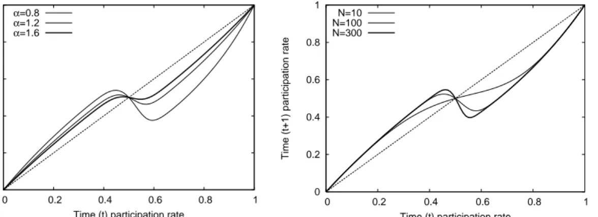
N=100 N=300
Figure 4: Graph of replicator dynamics (23) for three different values of α and N. Left panel: Map for three different values of α and N = 100. Right panel: Map for three different values
of N and α = 1. In both panels the other parameters are γ = 1
2, β = 2γ and b = 12.
In case of the replicator dynamics we obtain
xt+1 =
xt(αβ + p(xt; bN, N ) −γβ)
xt(p(xt; bN, N) − γβ) + αβ
, (23)
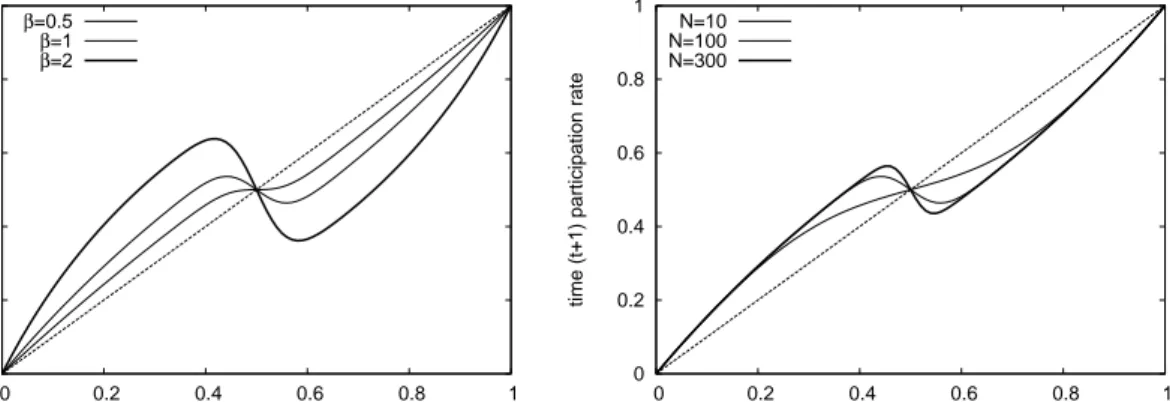
whereas under the adjusted logit dynamics we have
xt+1 = xtexp n β ³ p (xt; bN, N ) − γβ ´o xtexp n β ³ p (xt; bN, N) −βγ ´o + (1 − xt) . (24)
In both cases the dynamics can be described by a first order nonlinear difference equation
parameterized by N, b = Nc
N, α, β and γ. In the panels of Fig. 4 and Fig. 5 we plot (23) and
(24) for different values of the number of players N and the parameters α or β, respectively.
By Proposition 2, and as illustrated by Figs. 4-5, the three steady states are given by x∗ = 0,
0 0.2 0.4 0.6 0.8 1 0 0.2 0.4 0.6 0.8 1
time (t+1) participation rate
time (t) participation rate β=0.5 β=1 β=2 0 0.2 0.4 0.6 0.8 1 0 0.2 0.4 0.6 0.8 1
time (t+1) participation rate
time (t) participation rate N=10
N=100 N=300
Figure 5: Graph of adjusted logit dynamics (24) for three different values of β, keeping γ/β fixed, and N. Left panel: Map for three different values of β, keeping γ/β fixed and N = 100. Right panel: Map for three different values of N and β = 1. In both panels the other
parameters are β = 2γ and b = 1
2.
stability of these steady states it is convenient to define
δ (x; b, N) = ∂p (x; bN, N )
∂x .
Obviously δ (x; b, N ) < 0, since an increase in the fraction of agents participating always decreases the probability that less than bN of them indeed participate. Local stability analysis also requires that we make some assumptions on the derivatives of the switching function. In particular we make the intuitive assumption that for j, k = 0, 1 we have
∂ρjk(x, π) ∂xk ¯ ¯ ¯ ¯ xk=0,πk>πj > 0. (25)
That is, if the fraction using strategy k increases from zero, then more agents will move to that strategy. We also impose
∂ρjk(x, π) ∂+πk ¯ ¯ ¯ ¯ xk>0,πk=πj > 0 and ∂ρjk(x, π) ∂−πj ¯ ¯ ¯ ¯ xk>0,πk=πj < 0, (26)
where ∂+ and ∂− refer to right and left derivatives respectively.13 These assumptions imply
that, when payoffs are equal, an increase in the payoff differential increases the propensity to switch.
The following proposition characterizes stability of the steady states for our general class of evolutionary dynamics when all agents are either optimists or pessimists.
Proposition 3 Consider the participation rate dynamics given by (22) and suppose properties
(11)–(14) and properties (25)–(26) hold. Then the two boundary steady states x∗ = 0 and
x∗ = 1 are locally unstable. The interior equilibrium x∗ = s∗ is locally stable when both the
right derivative J+(s∗) = 1 + (1 − s∗) βδ∗ ∂ρ01 ∂+π1 ¯ ¯ ¯ ¯ x=s∗
13We need to use right and left derivatives because, due to property (12), the switching function ρ
jk has a
kink at πj = πk, and left and right derivatives are therefore not equal at that point (in particular, the right
and the left derivative J−(s∗) = 1 − s∗βδ∗ ∂ρ10 ∂−π1 ¯ ¯ ¯ ¯ x=s∗
are larger than −1, where δ∗ ≡ δ (s∗; b, N ).
It is now easy to apply the previous proposition for specific choices of switching functions satisfying (25)–(26), like those corresponding to the replicator or adjusted logit dynamics.
Applying Proposition 3 to both dynamics, and upon noticing that for both we have J+(s∗) =
J−(s∗) = J (s∗), we obtain the following result
Corollary 1 The interior steady state s∗ is locally stable for the replicator dynamics (16)
when
J(s∗) = 1 + s∗(1 − s∗)βδ∗
α > −1 (27)
and s∗ is locally stable for the adjusted logit dynamics (19) when
J(s∗) = 1 + s∗(1 − s∗) βδ∗ > −1 . (28)
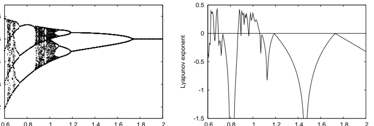
The stability conditions in Proposition 3 and Corollary 1 depend upon β, possibly α and,
through δ∗ and s∗, implicitly upon b and N. Fig. 6 shows the dynamics of x and the
corresponding Lyapunov exponent for different values of α for the replicator dynamics. For a high speed of adjustment (small α), an overshooting effect causes instability. As the speed of
adjustment decreases (i.e., as α increases) adaptation is slower and the equilibrium s∗ becomes
stable. The right panel of Fig. 6 indicates that there exist many values of α for which the
dynamics is chaotic, in the sense that it exhibits sensitive dependence upon initial conditions.14
Also note that the dynamics is invariant under a rescaling of the payoffs α, β and γ, implying that a unilateral increase from α to ϑα is equivalent with a change from β and γ to β/ϑ and
γ/ϑ, respectively. Fig. 6 therefore also illustrates the effect of a simultaneous decrease in β
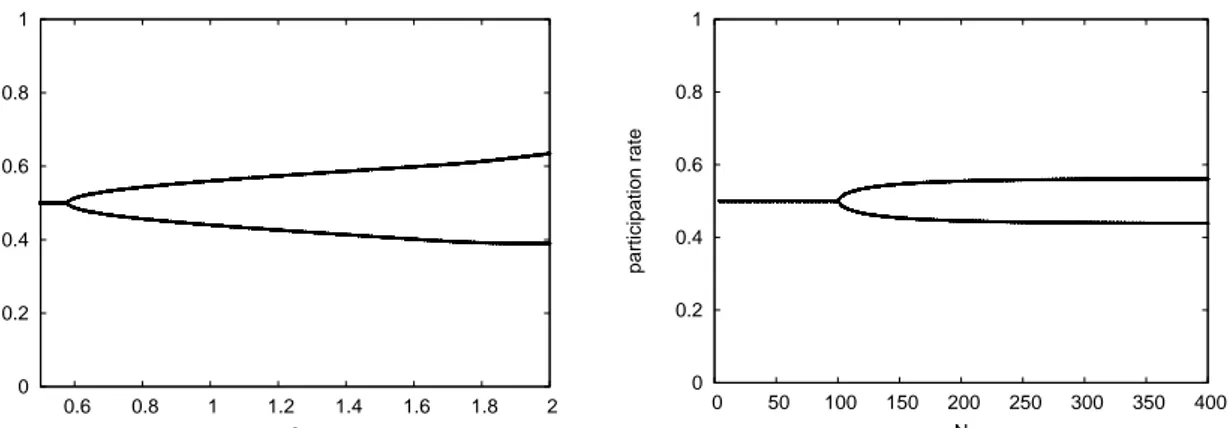
and γ. The left panel of Fig. 8 shows what happens in the adjusted logit dynamics when
β increases. Differently from the replicator dynamics case, when the interior steady state s∗
becomes unstable, the dynamics converges to a period two cycle for all values of β.
We are also interested in characterizing the stability of s∗ as a function of N, which affects
the stability both through s∗ and δ∗. The right panels of Fig. 4 and Fig. 5 already suggests
that s∗ becomes unstable for N large enough. The following proposition corroborates that.
Proposition 4 Let the dynamics of participation rates be given by (22). For any given value
of α, γ < β, and b the interior steady state s∗ is unstable when N → ∞. Moreover, if β = 2γ
and b = 1
2 there exists a unique M such that the steady state s∗ is locally stable if and only if
N < M.
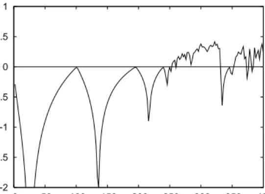
Fig. 7 shows the dynamics of x and the corresponding Lyapunov exponent for different values of N for the replicator dynamics, and the right panel of Fig. 8 shows the dynamics of x for
14The left panel of Fig. 6 also shows that for some parameter values (for example, for α ≈ 0.8) this
one-dimensional system has a 3-cycle which implies, by the Li–Yorke theorem (Li and Yorke, 1975) that the dynamics for those parameter values is chaotic.
different values of N for the adjusted logit dynamics. For small N the dynamics is stable
but as N increases an overshooting effect causes instability. Indeed Fig. 9 shows that J(s∗)
is decreasing in N and crosses the horizontal line with intercept −1 when N is larger than some threshold value M. This holds both for the replicator dynamics (left panel) and for the adjusted logit dynamics (right panel). The intuition behind Proposition 4 is that as N increases the average population payoff of the optimistic rule gets closer to the step payoff function of the underlying one shot game (see Fig. 4). As a result, for any value of the payoff
parameters, α, β > γ, as N increases (22) becomes steeper at the steady state s∗ and the
system loses stability. This dependence of the dynamics upon N is due to the assumption of
random matching. In fact, for N = 2 (with Nc = 1) the optimists payoff, π1, is linear in x,
since the probability of meeting a player who is using the pessimistic rule is p (x; 1, 2) = 1 − x. However, the probability of having less than half of the players participating when more than half of the other players are optimists, decreases as N increases. That is, as N increases (and for given b) the function p (x; bN, N ) will look more and more like a step function. We can therefore also interpret the parameter N as a measure of the shape and steepness of the payoff function at the steady state in a framework where all the (large) population of players play the same game. In that case a low value of N would give an optimists payoff function which decreases slowly as the number of participating players increases, similar to the linear one used in the market entry experiments (see, for example, Sundali et al., 1995). A high value of
N, on the other hand, would represent an expected payoff function close to the step function
used in the El Farol bar game, with payoffs at the symmetric MSNE dropping rapidly as an extra player participates.
0.2 0.3 0.4 0.5 0.6 0.6 0.8 1 1.2 1.4 1.6 1.8 2 participation rate α -1.5 -1 -0.5 0 0.5 0.6 0.8 1 1.2 1.4 1.6 1.8 2 Lyapunov exponent α
Figure 6: Replicator Dynamics. Left panel: Bifurcation diagram with respect to α. Right
panel: Lyapunov exponents for different values of α. Parameters values are b = Nc
N = 12,
N = 300, γ = 1
2 and β = 2γ. For every value of N, 100 iterations are shown after an
initialization period of 100.
Fig. 10 gives a specific example of the global dynamics of the replicator dynamics when the
steady state s∗ is locally unstable. The time series (left panel) looks aperiodic and indeed
the Lyapunov exponent for these values of the parameters is positive so that the dynamics exhibits sensitive dependence on initial conditions (see right panel of Fig. 6 at α = 1 or right panel of Fig. 7 at N = 300).
Even such a simple one-dimensional system is therefore able to produce complicated times series similar to those obtained by, e.g. the computational model of Arthur (1994). The evidence is gathered in the panels of Figs. 6-7. Clearly, as α decreases and/or N increases the
0 0.2 0.4 0.6 0.8 1 0 50 100 150 200 250 300 350 400 Participation rate N -2 -1.5 -1 -0.5 0 0.5 1 0 50 100 150 200 250 300 350 400 Lypunov exponent N
Figure 7: Replicator Dynamics. Left panel: Bifurcation diagram with respect to N. Right
panel: Lyapunov exponents for different values of N. Parameters values are b = Nc
N = 12,
α = 1, γ = 1
2 and β = 2γ. For every value of N, 100 iterations are shown after an initialization
period of 100.
dynamics of the participation rate x becomes unstable, after which a period-doubling route to chaos sets in, at least for the replicator dynamics. The right panels show that there exist values of both parameters where the Lyapunov exponents is positive implying sensitive dependence on initial conditions, a possible definition of chaotic behavior.
Finally, note that the influence of α, β and N on the dynamics is at odds with what should be expected if agents were repeatedly playing the MSNE of the one-shot game. First, increasing α destabilizes the dynamics in our model, although it does not have an impact on the equilibria of the one-shot game (see footnote 3 in Section 2). Second, fluctuations in the participant rate in our numerical simulations are increasing (or at least not decreasing) when the number of players N increases, whereas in Section 2 we have shown that at the symmetric MSNE the variance of the participation rate approaches zero as the number of players increases. Experiments with human subjects and different values of N and\or α may shed more light on the real relationship between these parameters and the size of the fluctuations, and thus on the validity of our model.
5
Exploiting participation fluctuations
In the previous section we have established that for a high speed of adjustment, a high intensity of choice, and/or for large N, the evolutionary competition between an optimistic and a pessimistic rule induces fluctuations of the aggregate participation rate x around the steady
state s∗. The right panel in Fig. 10 shows that there may be a significant correlation between
the participation rates and its lagged values. One might argue that the competition between the optimistic and pessimistic rule is not stable against the entrance of more sophisticated rules. The aim of this section is to investigate how the inclusion of such new rules affects the participation rate dynamics and whether they may succeed in exploiting these regularities. Similar analyses have been performed in Hommes (1998) and Brock et al. (2006) for the cobweb model. Most of our analyses in this section make use of the replicator dynamics (16) as updating mechanism, but we will also briefly discuss the results when fractions are updated according to the adjusted logit dynamics (19).
0 0.2 0.4 0.6 0.8 1 0.6 0.8 1 1.2 1.4 1.6 1.8 2 participation rate β 0 0.2 0.4 0.6 0.8 1 0 50 100 150 200 250 300 350 400 participation rate N
Figure 8: Adjusted Logit Dynamics. Left panel: Bifurcation diagram with respect to β, keeping the ratio γ/β fixed. Right panel: Bifurcation diagram with respect to N. Parameters
values are b = Nc
N = 12, N = 300, and β = 2γ. For every value of N, 100 iterations are shown
after an initialization period of 100.
-5 -4 -3 -2 -1 0 1 0 50 100 150 200 250 300 350 400 Jacobian at x=s * N α=0.6 α=1 α=1.5 -5 -4 -3 -2 -1 0 1 0 50 100 150 200 250 300 350 400 Jacobian at x=s * N β=0.6 β=1 β=1.5
Figure 9: Stability condition. Slope of (22), evaluated at x = s∗, as a function of N, for
two types of switching dynamics. Left panel: Replicator Dynamics. Right panel: Adjusted
Logit Dynamics. When not otherwise specified parameters are b = 0.5, β = 1 and α = 1.
Since there is a strong positive autocorrelation at the second lag, indicating ‘up-and-down’
behavior, a best response to predicting xt−2 for period t seems to be a sensible strategy. This
so-called “2-lags best reply” rule is given by15
p2,t = BR (xt−2) = 1 0 if xt−2 < b if xt−2 ≥ b . (29)
Generalizing this to three lags, four lags, or j lags best responders is straightforward. Letting
x2,t be the fraction of 2-lags best responders, the participation rate at time t is given as:
xt= x1,t+ x2,tBR (xt−2) ,
15The reader may wonder why we do not investigate a “1-lag best reply” rule. Since the interaction between
the optimistic and the pessimistic rule generates a strong first order negative autocorrelation in participation rates, one lag best responders are very often wrong in their prediction. Simulations confirm that these one lag best responders are quickly driven out.
0 0.2 0.4 0.6 0.8 1 0 20 40 60 80 100 Participation rate Time -1 -0.5 0 0.5 1 0 5 10 15 20 25 Autocorrelation Lag
Figure 10: Replicator Dynamics. Left panel: Participation rate time series. Right panel:
Autocorrelation diagram. Parameters values are N = 300, Nc = 150, α = 1, γ = 12 and
β = 2γ.
where x1,t and x0,t = 1 − x1,t− x2,t are the fractions of optimists and pessimists, respectively.
As before, the latter have payoffs α and expected payoff for optimists is given by π1,t =
α + βp (xt; Nc, N ) − γ. Expected payoffs for 2-lags best responders are:
π2,t = (1 − BR (xt−2)) α + BR (xt−2) π1,t.
Now let fractions x0,t+1, x1,t+1 and x2,t+1 evolve according to the replicator dynamics (16),
which is based upon payoffs generated by the different rules, which, in turn, depend upon xt
and xt−2. This leads to a four-dimensional dynamical system. The interior steady state of this
system is characterized by x = s∗. At x = s∗ every rule generates the same expected payoff.
If s∗ ≥ b the two lags best responders are not participating at the steady state. Therefore,
there is a continuum of steady state fractions with x∗
1 = s∗ and x∗0+ x∗2 = 1 − s∗.
Because the rule p2,t is discontinuous we rely on numerical simulations to determine local
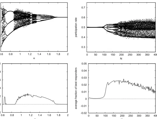
stability of these steady states. As illustrated in the upper panels of Fig. 11, the replicator dynamics with these rules is unstable and leads to persistent fluctuations in participation rates
for a high speed of adjustment (low α) and/or large N.16 The lower panels of Fig. 11 show
the time average of the fraction of 2-lags best responders along 100 iterations. This average
fraction approaches zero when the steady state s∗ is locally stable and is strictly positive
otherwise. With high α and small N the dynamics converges to the steady state x = s∗ along
a “shrinking” 3-cycle Along such a cycle a 2-lags best responder is more often wrong than
right in its prediction and slowly disappears. Note that, even if x2 approaches zero, it could
happen that the participation rate x settles at s∗ before x
2 equals zero. The simulations show
that this typically does not happen.
A different participation rate dynamics occurs when α is low and N large. In this case the dynamics is typically non-periodic and 2-lags best responders survive. Moreover the stable 2-cycles that existed when only optimists and pessimists are present have now disappeared. In fact, no 2-cycle could exist in this framework with 2-lags best responders. Assuming that a 2-cycle exists implies that the fraction of 2-lags best responders is either always increasing,
16 Simulations show that the instability threshold of both α and N are roughly the same as those fond in
the analysis of optimists vs. pessimists in Section 4. Back of the envelope computations for a continuous approximation of (29) show that, provided BR0(s∗) = 0, local stability of s∗ is still related to the conditions
0.2 0.3 0.4 0.5 0.6 0.6 0.8 1 1.2 1.4 1.6 1.8 2 participation rate α 0.3 0.4 0.5 0.6 0.7 0 50 100 150 200 250 300 350 400 participation rate N -0.02 0 0.02 0.04 0.06 0.08 0.1 0.6 0.8 1 1.2 1.4 1.6 1.8 2
average fraction of best responders
α -0.02 -0.01 0 0.01 0.02 0.03 0.04 0.05 0 50 100 150 200 250 300 350 400
average fraction of best responders
N
Figure 11: Replicator Dynamics. Evolutionary competition between optimists, pessimists and two lags best responders. Top left panel: Long run participation rate for different speeds of adjustment α. Bottom left panel: Time average (over 100 periods) of the fraction of 2-lags best responders for different values of α. The time average is computed along the iterations shown in the top left panel. Right panels: Same as above but with changing number of players N and fixed α. In all the cases b = 0.5 β = 2γ and γ = 0.5.
at the expense of both optimists and pessimists, or already equal to one. In the first case the 2-cycle is not stable, since fractions are changing, in the second case all agents are 2-lags best repliers so that the 2-cycle must be something like {0, 1, 0, 1, . . . }. But this is in contradiction with the 2-lags BR rule since when recording such a sequence the rule would predict that the next period few players will participate, thus suggesting to participate. This leads to 0, 1, 1, and therefore the 2-cycle is broken up.
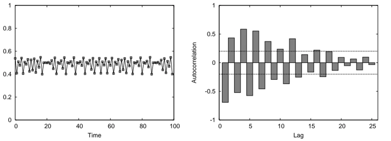
The absence of 2-cycles is also reflected in the autocorrelation structure of the chaotic dynam-ics. The upper left panel of Fig. 13 shows the participation rate for N = 300. Even though the time series is not periodic, the autocorrelation diagram (upper right panel of Fig. 13) shows that the autocorrelation at the second lag has indeed decreased substantially (and in fact is not significantly different from zero).
Despite the fact that 2-cycle behavior seems to have disappeared from the autocorrelation plot, the autocorrelation at the third lag is strongly positive, suggesting that the time series of participation rates has elements of a noisy 3-cycle.
This begs the question as to what would happen if a new rule that tries to exploit this feature
is introduced. To that end, we introduce the “3-lags best reply” rule p3,t = BR (xt−3). The
evolutionary competition of the four rules gives a six-dimensional dynamical system. Given
that s∗ ≥ b there is a continuum of steady states of the type x
1 = s∗ and x0+ x2+ x3 = 1 − s∗.
The steady state s∗ is unstable for low α and large N and leads to erratic participation rates,
0.2 0.3 0.4 0.5 0.6 0.7 0.6 0.8 1 1.2 1.4 1.6 1.8 2 participation rate α 0.3 0.4 0.5 0.6 0.7 0 50 100 150 200 250 300 350 400 participation rate N -0.02 0 0.02 0.04 0.06 0.08 0.1 0.6 0.8 1 1.2 1.4 1.6 1.8 2
average fraction of best responders
α Two lags BR Three lags BR -0.02 0 0.02 0.04 0.06 0.08 0.1 0 50 100 150 200 250 300 350 400
average fraction of best responders
N
Two lags BR Three lags BR
Figure 12: Replicator Dynamics. Evolutionary competition between optimists, pessimists, two and three lags best responders. Top left panel: Long run participation rate for different speeds of adjustment α. Bottom left panel: Time average (over 100 periods) of the fraction of 2-lags best responders for different values of α. The time average is computed along the iterations shown in the top left panel. Right panels: Same as on the left but with changing number of players N and fixed α. In all the cases b = 0.5 and β = 2γ.
0 0.2 0.4 0.6 0.8 1 0 20 40 60 80 100 Participation rate Time -1 -0.5 0 0.5 1 0 5 10 15 20 25 Autocorrelation Lag 0 0.2 0.4 0.6 0.8 1 0 20 40 60 80 100 Participation rate Time -1 -0.5 0 0.5 1 0 5 10 15 20 25 Autocorrelation Lag 0.3 0.4 0.5 0.6 0.7 0 20 40 60 80 100 participation rate time -1 -0.5 0 0.5 1 0 5 10 15 20 25 autocorrelation lag 0 0.2 0.4 0.6 0.8 1 0 20 40 60 80 100 Participation rate Time -1 -0.5 0 0.5 1 0 5 10 15 20 25 Autocorrelation Lag
Figure 13: Replicator Dynamics. Upper panels: Participation rate and autocorrelation diagram for competition between optimists, pessimists and 2-lag best responders. Middle-Upper panels: Participation rate and autocorrelation diagram for competition between op-timists, pessimists two and three lag best responders. Middle-Lower panels: Participation rate and autocorrelation diagram for competition between optimists, pessimists two, three and four lag best responders. Lower panels: Participation rate and autocorrelation diagram for competition between optimists, pessimists and two to six lag best responders. The dotted lines show the 5% significance levels of the autocorrelations. Autocorrelations and significance
levels are based upon a sample of 100 observations. Parameters values are N = 300, b = 1
2,
0.3 0.4 0.5 0.6 0.7 0 20 40 60 80 100 participation rate time -1 -0.5 0 0.5 1 0 5 10 15 20 25 autocorrelation lag 0.25 0.3 0.35 0.4 0.45 0.5 0.55 0.6 0.65 0.7 0 20 40 60 80 100 participation rate time -1 -0.5 0 0.5 1 0 5 10 15 20 25 autocorrelation lag 0.3 0.4 0.5 0.6 0.7 0 20 40 60 80 100 participation rate time -1 -0.5 0 0.5 1 0 5 10 15 20 25 autocorrelation lag 0.3 0.4 0.5 0.6 0.7 0 20 40 60 80 100 participation rate time -1 -0.5 0 0.5 1 0 5 10 15 20 25 autocorrelation lag
Figure 14: Adjusted Logit Dynamics. Upper panels: Participation rate and autocorrelation diagram for competition between optimists, pessimists and 2-lag best responders. Middle-Upper panels: Participation rate and autocorrelation diagram for competition between op-timists, pessimists two and three lag best responders. Middle-Lower panels: Participation rate and autocorrelation diagram for competition between optimists, pessimists two, three and four lag best responders. Lower panels: Participation rate and autocorrelation diagram for competition between optimists, pessimists and two to six lag best responders. The dotted lines show the 5% significance levels of the autocorrelations. Autocorrelations and significance
levels are based upon a sample of 100 observations. Parameters values are N = 300, b = 1
2,