Branch and Bound pattern in FastFlow

(1)

Departments of Computer Science and Information Engineering

AND

SCUOLA SUPERIORE SANT' ANNA

Master Programme in Computer Science and Networking

Master Thesis:

Branch and Bound pattern in FastFlow

Candidate: Cecchi Gian Luca

Supervisor:

Prof. Marco Danelutto

(2)

(3)

efforts she has made and that made

it possible to achieve this goal.

With the commitment that this

milestone is only the starting point

for many other dreams that now,

thanks to her, I can try to achieve

alone.

(4)

(5)

1 Introduction...13

2 Structured Parallel Programming...19

2.1 Farm Skeleton...21

2.2 FastFlow...24

3 Branch and Bound Algorithm...27

3.1 Constrained Shortest Path ...31

3.1.1 Solving the Constrained Shortest Path problem...33

3.1.2 Example of Constrained Shortest Path problem...34

3.2 Parallel Branch and Bound...38

4 B&B logical implementation...41

5 Code Implementation: B&B skeleton...45

5.1.1 Tree node class...46

5.1.2 Branch and Bound class...47

5.1.3 Emitter class...49

5.1.4 Worker class...51

6 Test applications...53

6.1 Vettore class...53

6.2 Link and Nodo classes...54

6.3 Graph class...55

6.4 Main class CSP test application...57

6.5 Main class synthetic application...59

7 Experimental results...63

7.1 Synthetic application performance...64

7.1.1 Measured Times...66

7.2 CSP test application performance...76

7.2.1 CSP sequential performance...76

7.2.2 Parallel CSP application performance...79

8 Conclusions...85

(6)

(7)

Figure 1: Farm skeleton schema...24

Figure 2: Farm with feedback schema...26

Figure 3: Layered FastFlow design...27

Figure 4: Simple flowchart on the Branch and Bound algorithm...30

Figure 5: Graph of the starting problem P...37

Figure 6: Graph of the problem P1...38

Figure 9: Branch and Bound tree for the example reported in section 3.1.2...40

Figure 10: Graphical view of a parallel Branch and Bound algorithm...43

Figure 11: Branch & Bound skeleton UML diagram...47

Figure 12: Intel® Xeon® Processor E5-2650 specifications...65

Figure 13: Completion time of the 3 – 100 – 10 – 6 configuration...69

Figure 14: Speed-up of the synthetic application with configuration 3 – 100 - 10 – 6...70

Figure 16: Speed-up of the synthetic application with configuration 50 – 50 – 10 – 6...71

Figure 18: Speed-up of the synthetic application with configuration 50 – 10 - 10 – 6...73

Figure 24: Speed-up of the synthetic application with configuration 10 – 100 – 2 – 19....77

Figure 25: Ideal completion time graph of the CSP application...80

Figure 26: Ideal mean time per task graph of the CSP application...80

Figure 27: Speed-up based on Completion time...82

Figure 28: Completion time graph...82

Figure 29: Mean time per task graph...83

Figure 30: Speed-up based on mean time per task values...84

(8)

(9)

Code 1: Branch and Bound pseudo-code for a minimization problem...29

Code 2: Dijkstra pseudo-code algorithm...32

Code 3: Minimum Cost Flow problem formulation...32

Code 4: Shortest Path and Constrained Shortest Path formulations...33

Code 5: bb_tree_node class...46

Code 6: ff_bb class...48

Code 7: bbEmin class...50

Code 8: Termination condition...51

Code 9: bbW class...52

Code 10: Vettore class...54

Code 11: Example of instantiation of a Vettore with the ff_allocator...54

Code 12: Header of the Link class...55

Code 13: Header of the Nodo class...55

Code 14: Header of the Graph class...56

Code 15: file format for populating the graph with the Grafo(const char* s) constructor. .56 Code 16: first lines of the file used to populate the graph in the tests performed ...57

Code 17: TreeNode class of the CSP application...58

Code 18: main method in the main.cpp file of the CSP application...59

Code 19: main.cpp file of the synthetic application...60

Code 20: branch() and solve() method of the synthetic application...61

Code 21: Grafo.h...89 Code 22: Grafo.cpp...92 Code 23: Link.h...92 Code 24: Link.cpp...93 Code 25: Nodo.h...93 Code 26: Nodo.cpp...94 Code 27: Vettore.h...96 Code 28: Path.h...96 Code 29: Path.cpp...98 Code 30: B&B.hpp...107 Code 31: Main.cpp...111

Code 32: File used to instantiate the graph in the CSP test application...116

(10)

(11)

Table 1: Configuration 3 – 100 – 10 – 6 performance...67

Table 7: Ideal completion time...77

Table 8: Parallel Branch and Bound completion time comparison...79

Table 9: Mean time per task comparison...81

(12)

(13)

1 I

NTRODUCTION

he thesis aim was to develop a Branch and Bound parallel framework [14] [15] implemented as a skeleton to be added to the existing skeletons in the FastFlow parallel framework environment [22].

T

FastFlow is a C/C++ programming framework supporting the development of pattern-based parallel programs on multi/many-core and distributed platforms. It is implemented as a template library and may be used to parallelize an application using a structured parallel programming methodology. This methodology is based on the use of recurrent schemas of parallel computation suitable to support many application and algorithm called patterns or skeletons [1] [20] [21].

The focus of the thesis is to investigate the feasibility of a FastFlow implementation of a Branch and Bound pattern.

Branch and Bound [9] [11] [14] [15] is a general algorithm for finding optimal solutions of various optimization problems. It is used to solve problems of different type including problems over graphs like the Constrained Shortest Path (CSP) problem [23] or the Travelling Salesman problem (TSP). The Branch and Bound algorithm implementation is based on the divide and conquer schema that is a well known technique in computer science stating that if a problem is too hard to be solved it is convenient to subdivide the problem in smaller sub-problems, in such a way solving the sub-problems gives also the solution to the starting problem. In this way the Branch and Bound algorithm splits more and more the problem to be solved up to the point it obtains easy-to-solve sub-problems. These sub-problems are solved and the solutions used to compute the solution to the original problem. A Branch and Bound algorithm consists of a systematic enumeration of all candidate solutions, where large subsets of fruitless candidates are pruned, by using

(14)

upper and lower estimated bounds of the quantity being optimized.

The final guidelines were to develop a skeleton implementing a Branch and Bound parallel framework that may be specialized by the user to solve the kind of problems solvable with a Branch and Bound approach. To achieve this goal the skeleton has been implemented leaving to the users the task of providing the application specific code and all the objects needed to implement the Branch and Bound framework. In particular some method is programmed inside the skeleton as abstract function. This means that the client of the skeleton must write a concrete implementation for this functions in order to be able to use the skeleton. Two important abstract functions in the skeleton are the solve() function and the branch() function, the solve() function is needed to evaluate each problem in the B&B algorithm, the branch() function is needed to split a problem in sub-problems implementing the divide and conquer step. These functions strictly depend on the kind of problem the client wants to solve and therefore the choice to model these functions as abstract functions was the only possible choice.

The implementation of the B&B skeleton is built on top another pattern already present in the FastFlow library, that is the Farm with feedback [1].

The Farm skeleton consists on the replication of a pure function, without knowing the internal structure of the function itself. It is commonly implemented using an Emitter, one or more Workers and a Collector. The Emitter is in charge of scheduling input data elements to one of the Workers. The Workers are in charge of computing the replicated pure function over the received data element from the Emitter. The Collector collects the results coming from Workers and sends these results on the output stream of the Farm.

The Farm with feedback differs from the standard Farm paradigm in the fact that it has not a Collector module and every Worker has a feedback channel with the Emitter. The Workers send back the results to the Emitter after the completion of the replicated function through the feedback channel. In this case there is no output channel, but results are usually processed by the Emitter module.

The Farm with feedback skeleton fits in an efficient and elegant way the needs of divide and conquer problem types thanks to its feedback channel that allows to build a master/worker schema where the master organizes the workers jobs and the workers execute in parallel the problems them assigned by the master. In case of a Branch and

(15)

Bound algorithm the master may be used to split the problems and to schedule the sub-problems to the workers and the workers may be used to compute each sub-problem in parallel and to send the solved sub-problems back to the master. A possible implementation of the Farm with feedback skeleton uses two type of modules: an Emitter module and one or more Workers modules. The Emitter implements the role of the master while the Workers implement the role of the workers.

The Emitter is in charge of calculating and storing the values needed to compute the interval of interest for the algorithm and to use it to decide the pruning cases for each problem. Moreover the Emitter executes the branch() function, the function that splits a problem in sub-problems, over the problems that were not pruned in the previous control phase. The Workers are in charge of executing the solve() function for each problem received from the Emitter. After the completion of this function the problem analysed is sent back to the Emitter through the feedback channel and then this problem will be either pruned or branched by the Emitter.

Before testing the developed skeleton we proposed a simple cost model deriving it from the cost model of the Farm skeleton and using the structured parallel programming theory [1] [20] [21]. This cost model states that the skeleton completion time, assuming that there are no bottlenecks, is # tasks×T_W/nw , where TW is the service time of the

Workers, nw is the number of Workers of the skeleton and #tasks is the number of tasks executed during the computation of the skeleton. The only module that may be a bottleneck is the Emitter, and it is a bottleneck if T_E/num>T_W/nw , that is if the service time of the Emitter (TE) over the mean number of sub-problems that the branch() function

generates (num) is greater than the service time of the Workers (TW) over the number of

Workers of the skeleton (nw). In case the Emitter is a bottleneck the completion time becomes # tasks×T_E/num.

To analyse the performance of the skeleton, we developed two test applications and we measured the performance attained by their execution. The test applications developed are: a synthetic application that may be used to simulate others real application computations and an application solving the Constrained Shortest Path problem.

The synthetic test application we developed allow us to easily change the key parameters (from a computational point of view) of the problem represented. This

(16)

application is not aimed at solving a real problem, but it may be used to emulate the behaviour of real problems computed with this skeleton. This application is used to analyse the performance of the skeleton in different configurations. The parameters that can be changed in this application are: the completion time of the solve() function, the completion time of the branch() function, the number of sub-problems that the branch() function generates and the level of the Branch and Bound Tree where the problems are pruned. With the last two parameters it is possible to vary the total number of tasks that the algorithm generates. This application is also suitable to verify the proposed cost model and to analyse the required characteristic that the application we want to parallelize must have in order to achieve good performances.

The Constrained Shortest Path problem consists in finding the shortest path in an oriented and weighted graph that satisfies an additional constraint. In this thesis the additional constraint used is that the solution must contain less than L links. This problem is NP-hard and it's solvable with a Branch and Bound approach.

The results obtained are interesting: with both the test applications used we show that, under certain assumptions, it is possible to achieve performances very close to the ideal ones and it is possible to further optimize the skeleton to achieve even better performances [19]. We show that the skeleton scales as expected with all the configurations and applications tested. The only constraint outlined is that the Emitter should not to be a bottleneck as stated in the cost model proposed. This is a reasonable constraint also valid for the Farm paradigm.

The thesis is structured as follows: in the first part (sections 2,3) a summary of the background information needed to understand the thesis work is reported, in the second part (sections 4,5,6,7) the design development decision and the code implementation of the thesis project are reported and the performance obtained from the tests application are analysed. More in detail, the section 2 summarizes the basic concepts of the structured parallel programming, the methodology used to develop the pattern. Section 3 analyses the Branch and Bound algorithm and the Constrained Shortest Path problem and its resolution through the B&B approach. Section 4 reports the logic implementation of the skeleton and the development decision taken. Section 5 reports the developed code to implement the B&B skeleton. Section 6 reports the code developed to implements the test applications.

(17)

Section 7 reports the experimental results obtained executing the test applications developed. The last two sections (8 and ) report respectively the conclusions over the thesis project and the appendices where it is possible to find the whole code for the skeleton and the test application.

(18)

(19)

2 S

TRUCTURED

P

ARALLEL

P

ROGRAMMING

Currently, an important technological evolution is ongoing: multi-manycore components, or chip multiprocessors, are replacing uniprocessor-based CPUs. The so called “Moore law” - according to which the CPU clock frequency doubles about every 1.5 years - since 2004 has been reformulated in: the number of cores (CPUs) on a single chip doubles every 1.5 years. This fact has enormous implications on technologies and applications: in some measure, all hardware-software products of the next years will be based on parallel processing. [1]

he evolution of the hardware architecture requires a new methodology for application development that must exploit the maximum potential of the new architectures executing in parallel processes and/or threads that cooperate to the resolution of a single problem. The “old” methodology, optimized for the execution of a program on a single-core machine, turns out to be inefficient on the new hardware architecture. For this reason it becomes of fundamental importance to develop applications that exploit more cores at the same time. Currently the most common method adopted to achieve this goal is to develop applications using sequential languages and message-passing or shared-memory libraries. This kind of programming, however, requires a considerable effort to synchronize and coordinate the processes/threads composing the program. To reduce the complexity of the parallelization problem higher level programming tools are necessary. An advanced approach is based on the concept of parallel patterns, also called parallel paradigms, or algorithmic skeletons. This approach consists in a higher-level programming methodology that provides the programmer with precise paradigms, or skeletons, implementing recurrent schemas of parallel computation suitable to support many applications and algorithms. These skeletons implement themselves all the operations needed to coordinate and synchronize the involved processes/threads, leaving to the programmer the only task of choosing the skeleton that better fits his needs and developing and providing the application-specific (business) code.

T

(20)

According to [1], algorithmic skeletons can be divided in two broad classes:

1. Stream-parallel skeletons are skeletons operating on independent data items appearing onto input streams. The mains stream-parallel skeletons are:

• Farm: it consists on the replication of a pure function, without knowing the internal structure of the function itself. It is commonly implemented using an Emitter, several Workers and a Collector. The Emitter is in charge of scheduling input data elements to one of the Workers. The Workers are in charge of computing the replicated pure function over the received data elements from the Emitter. The Collector collects the results coming from Workers and sends these results on the output stream of the Farm.

• Pipeline: it requires some knowledge of the form of the sequential computation. The sequential computation must be expressed as the composition of n functions: F( x)=Fn(F_n−1(... F2(F1(x ))...)). In this

case, a possible parallelization is a linear graph of n modules, also called pipeline stages, each one corresponding to a specific function.

• Data-flow: given a sequential computation, a partial ordering of operations is built through the computation-wide application of Bernstein conditions. The precedence relations express the strictly needed data dependences. The partial ordering is represented by a data-flow graph, that is the computation graph in this model.

2. Data-parallel skeletons operate on partitions of a collection. Usually these data are partitions of a single value and each single partition is computed in parallel by different processing unit.

• Map: it is the simplest data-parallel computation. It is commonly composed by a Scatter module, several Workers modules, and a Gatherer module. Input data are distributed through the Scatter that divides a single data value into more partitions and sends them to the Workers. Workers operates on its own local data only executing the replicated function F. Output data is collected through a Gather.

(21)

A[M] and to any associative operator ○, returns the following scalar value x=reduce( A , ∘)= A[0]∘ A [1]∘...∘ A [M−1]. Given that the operator is associative, the operations reported can be executed in parallel two by two. Therefore in a first phase the skeleton executes in parallel the following operations: A [0]∘ A[1] || A [2]∘ A [3] || ... || A [M−2]∘ A [M−1]. In the second phase the operator ○ is again used to compute two by two the results coming from the first phase and so on up to remain with a single value that is x.

• Stencil: is a more complex, yet powerful, computations characterized by Workers that operate in parallel and cooperate with data exchange. Data dependences are imposed by the computation semantics. A stencil is a data dependence pattern implemented by inter-worker communications.

With parallel programming is possible to drastically reduce the execution time of an operation or of a set of operations (in the case of execution on data streams). The performance available with this new methodology and architecture solicited the interest of the computer science community to focus on the resolution of problems that with a single core CPU are not tractable, like well known NP-Hard problems. The execution time of such problems may be greatly reduced using more processing units. In this thesis only the Farm skeleton, that is used in the thesis project, will be presented.

2.1 Farm Skeleton

Given a data stream xn , … , x1 the Farm skeleton computes F(xn), … , F(x1) in

parallel. This skeleton, in practice, consists in a pure replication of a function inside different modules that are executed in parallel.

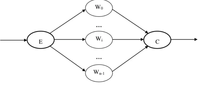
In Figure 1 a possible implementation of the Farm skeleton schema is reported. Three different modules types are recognizable: the Emitter (module E), the Workers (modules W0,...,Wn-1) and the Collector (module C). The execution flow is as follows: an

input stream serves the Emitter that provides to schedule each input data to one of the Workers. There are several scheduling mechanism, but the relevant feature is that this scheduling should balance the Workers load in such a way that each Worker should not be over-loaded or under-loaded with respect to the others in the Farm. A function F is

(22)

replicated in a set of identical modules: the Workers. Each Worker receives an input data from the Emitter and computes the function F on this input. After the completion of this function the result is sent on the output channel to the Collector.

The Collector serves as an output interface: collects the results coming from Workers and sends these results on the output stream of the Farm. The Emitter and Collector may be implemented in many ways, for example they may be implemented by the same module or by a tree structure; by now let's suppose that they are two single, distinct modules.

The advantages of using this skeleton are that a good load balancing among Workers can be easily obtained and no information are needed about the function that we want to parallelize. A constraint is that the Workers can't easily contain internal states and in case of frequent changes of this hypothetical internal state the Farm itself becomes unsuitable to parallelize the application. In fact in case of an internal state in the Workers there must be a mechanism that keeps all the state in all the Workers consistent. This mechanism may be implemented in different ways, but it is anyway time consuming. Frequent changes of a state in one of the Workers cause a frequent execution of this mechanism and therefore an hight amount of time is spent in this procedure, slowing the whole skeleton computation.

(23)

Using a Farm the execution time of a stream of tasks can be greatly reduced. To prove this assertion it's possible to briefly analyse its cost model [1]. The service time of the Worker is equal to the calculation time of the function F plus the time to send the result to the Collector: T_w=T_F+T_com. In case the underlying system may overlap communication time and computation time then T_com=0 and T_w=T_F. The service time of the Emitter and Collector can be assumed to be equal to the communication latency TE=TColl=Lcom. If the inter-arrival time to the Emitter is TA, the optimal

parallelism degree, that represents the optimal number of Workers for the given problem, is n_opt=

_⌈

T_calc/T_A

_⌉

and, assuming that in the farm there are no bottlenecks, the Farm service time is T_Farm=T_w/n . This means that every T_Farm seconds a task result will be sent onto the output stream by the Collector. To execute the function F on a stream of 100 tasks the Farm would take (T_F/n)×100 seconds, while in a sequential program the same application would take 100×T_F seconds. It's easy to observe that the Farm introduced a theoretical speed-up of n.

Other important parallel programming measures are the speed-up and the efficiency. The speed-up provides a measure of the relative “speed” of the parallel computation with respect to the sequential one: if the best achievable completion time by the sequential application takes TAPP time to complete the execution and the parallelized

version takes TPAR , the speed-up index is s=TAPP/TPAR. The efficiency instead indicates

how much the effective performance differs from the ideal one and it is defined as

ε=s /n where n is the parallelism degree of the application.

In this thesis a particular type of Farm called Farm with feedback is used. This Farm differs from the one presented above in the fact that it has not a Collector module and every Worker has a feedback channel with the Emitter. Workers send back the results after the completion of the function F through the feedback channel. With this structure the execution flow goes as follows: the Emitter receives an input task from the input stream and schedules the task to a Worker. The Worker receives the task from the Emitter, computes the function F on the task and sends back to the Emitter the result of the computation through the feedback channel. In this case there is no output channel, but a result is usually updated in the Emitter module.

(24)

2.2 FastFlow

FastFlow aims to provide a set of low-level mechanisms able to support low-latency and high-bandwidth data flows in a network of threads running on a SCM. These flows, as typical in streaming applications, are supposed to be mostly unidirectional and asynchronous. [2]

FastFlow is the programming framework environment, developed at the Department of Computer Science of Pisa and Torino used to develop the thesis project. It is a C/C++ programming framework supporting the development of pattern-based parallel programs on multi/many-core and distributed platforms. It has been designed to provide programmers with efficient parallelism exploitation patterns suitable to implement stream parallel applications.

The whole programming framework has been developed on top of Pthread/C++ standard.

Streaming networks in FastFlow are build upon two lower-level companion concepts: lock-free Multiple-Producer-Multiple-Consumer queues and a parallel lock- free memory allocator. Both are realised as specific networks of threads connected via lock-free Single-Producer-Single-Consumer queues [3], which admit a very efficient implementation on cache-coherent Single Chip Multiprocessor. These concepts are implemented as a template library designed as a stack of layers that progressively abstracts out the

(25)

programming of parallel applications. This implementation has been designed to achieve portability, extensibility and performance.

In addition to the common patterns that characterize the structured parallel programming this library contains useful tools for the general parallel programming methodology, such as the ff_allocator.

The ff_allocator allocates only large chunks of memory, slicing them up into little chunks all with the same size. Only one thread can perform malloc operations while any number of threads may perform frees using the ff_allocator. The ff_allocator is based on the idea of Slab Allocator, for more details about Slab Allocator please see: Bonwick Jeff. The Slab Allocator: An Object-Caching Kernel Memory Allocator [4]. (M. Torquati in FastFlow: allocator.hpp [5])

The ff_allocator, as suggested by its name, is an extremely powerful allocator that can be used to allocate memory space to create objects or variables instead of using the normal constructs of C++ like the new operator and/or malloc. There is not available documentations about this allocator, but it is based on the idea of Slab Allocator.

A Slab Allocator acts as a normal allocator with the difference that when a chunk of memory is going to be freed it is not released but it is kept inside the allocator. In this way when another request for allocating space arrives to the allocator, if there is an available

(26)

free chunk of memory inside the allocator of the same size of the request this is returned to the requester without the intervention of the Operating System.

More documentations about FastFlow can be found in the online web-site [22]: [2] [3] [6] [7] [8].

(27)

3 B

RANCH

AND

B

OUND

A

LGORITHM

ranch and Bound is an algorithmic approach, used to solve NP-Hard problems, commonly based on the divide and conquer schema. Divide and conquer is a well known technique in computer science based on the concept that if a problem is too hard to be solved it is convenient to subdivide the problem in smaller sub-problems, in such a way solving the sub-problems gives also the solution to the starting problem. This method can be recursively applied to the problems. In that case the sub-problems will be further subdivided in smaller sub-problems and this procedure can be repeated until an easy-to-solve problem is encountered. Proceeding in this way a Branch and Bound Tree is created where the root is the starting problem and every node corresponds to a sub-problem.

B

This Algorithm is commonly used to solve problems like Binary Knapsack, Constrained Shortest Path and Travelling Salesman problem. In the thesis project the application implemented to test the parallel Branch and Bound performance executes the Constrained Shortest Path algorithm over a graph of 259 nodes.

Synthetically, the Branch and Bound paradigm could be summerized as follows:

Building the Branch and Bound Tree:

• A branching scheme splits a problem P into smaller and smaller sub-problems, in order to end up with easy-to-solve problems. Branch and Bound Tree nodes represent the sub-problems, while Branch and Bound Tree edges represent the relationship linking a parent-sub-problem to its child-sub-problems created by branching. The branching scheme must be designed in such a way it satisfies the Completeness property: every solutions, also non-optimal once, available in the problem P must be present in at least one of the sub-problems.

(28)

Completeness property:

Given the problem P and its subdivision by branching P1,P2,...,Pn and given the

solutions sets S,S1,S2,...,Sn to the problems P,P1,P2,...,Pn the branch scheme must

satisfy the following property: S=S1∪S2∪...∪Sn

Additional, not necessary properties of the branching scheme are: ◦ Partitioning: S_i∩S_j=∅, ∀ i≠ j

◦ Balancing:

∣

S_i

∣

≃

∣

S_j

∣

, ∀ i≠ j

• A search or exploration strategy selects one node among all pending nodes according to priorities defined a priori. The priority of a problem Pi is usually based

either on the depth of the node in the Branch and Bound tree or on its presumed capacity to yield good solutions. The first case leads to a depth-first tree-exploration strategy, if an higher priority is assigned to deeper nodes, or to a

(29)

first tree-exploration strategy, if an higher priority is assigned to shallower nodes. The second case leads to a best-first strategy.

Pruning Branches

• A bounding function F gives a lower bound for the value of the best solution belonging to each node or problem Pi created by branching.

• Upper bound and lower bound are used to create an interval that restricts the size of the tree to be built: only nodes whose evaluations belong to this interval are explored, other nodes are pruned. The upper bound (value of the best known solution) is constantly updated, every time a new feasible solution is found.

• Dominance relationships may be established in certain applications between sub-problems Pi, which will also lead to prune non dominant nodes.

A Termination Condition

This condition states when the problem is solved and the optimal solution is found. It happens when all sub-problems have been either explored or eliminated.

Procedure B&B (P, z) : begin Q:=(P); z:=+∞ ; repeat P' :=NEXT (Q);Q :=Q ∖{ P' }; zl:=RELAX (P '); if z_l<z then begin zu :=HEURISTIC (P '); if zu <z then z :=zu; if zu >zl then Q:=Q∪BRANCH (P '); end until Q=∅ end

Code 1: Branch and Bound pseudo-code for a minimization problem.

In Code 1, using a pseudo-code, a possible representation of the Branch and Bound algorithm is reported [9].

(30)

• NEXT(Q): The NEXT method selects a problem P' among the pending problems in Q. This method, as stated previously, can be implemented following more strategy depending on the problem to solve.

• RELAX(P'): The RELAX method calculates a lower bound value for the problem P'. This method is usually implemented via a relaxation approach that simplify the problem to be solved deleting or modifying some “problematic” constraints of the problem. Solving the relaxed problem is usually easy and gives a lower bound, in the case of a minimization problem, or an upper bound, in case of a maximization problem.

• HEURISTIC(P'): The HEURISTIC method calculates an upper bound value for the problem P'. This method is usually implemented using an heuristic specific to the type of problem addressed.

• BRANCH(P'): The BRANCH method is executed only when necessary: it is executed only in case that the current problem is not pruned by the algorithm. This method splits the problem P' in more sub-problems that are added to the set Q containing all the pending problems.

The logic of the algorithm is the following: it selects a problem P' among the pending problems in Q, it calculates lower and upper bounds to P' and if the found solution is feasible for the starting problem and it is the best solution found up to this point by the algorithm it is stored. Then P' is split in smaller sub-problems and these sub-problems are added to Q.

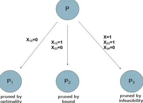
To avoid to analyse every problem of the Branch and Bound Tree the problems can be pruned. This happens in three cases: when the solution found by the HEURISTIC method is optimal for the selected problem P' (zu_{in Code 1) it's possible to avoid a further}

split, in this case the problem is pruned by optimality. When the problem P' has no admissible solutions (S'=Ø) it is useless to further split it, in this case the problem is pruned by infeasibility. If the lower bound found for the problem P' (zl in Code 1) is greater

than the current minimum upper bound found up to now for the starting problem P by the algorithm (z in Code 1), this means that in the selected problem P' there will not be optimal solutions for P, the problem is pruned by bounds.

(31)

3.1 Constrained Shortest Path

The Constrained Shortest Path problem derives from the simpler Shortest Path problem with the addition of one constraint. In this case the additional constraint is on the maximum number of links that the solution can contain. The Shortest Path problem is usually solved with algorithms based on the Dijkstra algorithm [10] [16] [17]. An efficient solution to this problem is reported by G. Gallo and S. Pallottino in Shortest Path Algorithms [10]. In this thesis is reported only briefly the Dijkstra algorithm because the focus of the thesis is not on the performance of this algorithm itself, but on the speed-up gained running the algorithm on the Branch and Bound parallel framework developed.

In Code 2 is reported the pseudo-code of the Dijkstra algorithm. This algorithm calculates in polynomial time the shortest distance between a source node and all the other nodes in the graph and the paths that gives this value. The returned values of this algorithm are the vectors dist and prev : the first vector is constructed in such a way the ith position of the vector contains the shortest distance between the source and the ith node of the graph (dist[i] = shortest distance between source node and node i). The second vector is used to specify which is the shortest path from the source and the ith node. The reconstruction of the path using the vector prev is tricky: every position i of the vector contains the previous node in the shortest path between the source and the node i. Assuming a prev vector populated in this way [ 0 | * | * | 0 | * | 3 | * | * | 5 | * | * | * | 8 ] the shortest path between the node 0 and the node 12 is calculated as follows: the last node of the path is set equal to 12, to know the previous node in the path the prev vector is checked, in particular the value stored in prev[12] gives the previous node of the path that in this case is 8. In pre[8] it's possible to discover the antepenult node of the paths that is 5. This procedure is repeated until the node found in the prev vector is the source node, at this point the path is complete, in this case it is [ 0→3→5→8→12 ].

function Dijkstra(Graph, source):

For each vertex v in Graph: dist[v] := +∞ ;

prev[v] := undefined ;

end for dist[source] := 0 ;

(32)

while N not empty:

u := vertex in N with smallest distance in dist[] ; remove u from N ;

if dist[u] = +∞ :

break ; end if

For each neighbour v of u: alt := dist[u] + dist_between(u, v) ; if alt < dist[v]: dist[v] := alt ; prev[v] := u ; decrease-key v in N; end if end for end while

return pair(dist , prev);

Code 2: Dijkstra pseudo-code algorithm

With the addition of the constraint on the maximum number of links that the solution can contain the problem becomes NP-Hard, and can be solved using the Branch and Bound algorithm. The Constrained Shortest Path problem can be formulated as a special case of the Minimum Cost Flow problem [11] :

Let G=(N , A)be a direct network N set of n nodes

A set of m directed arcs

cijcost perunit flow on(i , j), ∀ (i, j)∈A

uijcapacity of (i, j), ∀(i , j)∈A

b(i)∈ℤ , supply /demand of node i ,∀ ∈N

b(i)>0 supply node b(i)<0 demand node b(i)=0 transit node xijdecision variables: flow to push along(i, j), ∀(i , j)∈ A

FS(i)set of the outgoing links from node i BS (i)set of theincoming links to node i Minimum Cost Flow :

Min

_∑

(i, j )cij∗xij

•

∑

₍_{ij)∈FS (i )}x_ij−

∑

(ji)∈BS (i)xji=b(i),∀ i∈N

• 0<x_ij<u_ij

•

∑

_{i∈ N}b(i)=0

(33)

The Shortest Path problem is a special case of the Minimum Cost Flow problem formulated in Code 3, where b(s)=1,b (d )=−1 and b(i)=0, ∀ i≠s ,d ∈N. The Constrained Shortest Path problem can be formulated imposing an additional constraint as showed in Code 4.

Shortest Path problem:

Let s be the source node and d the destination node

Min

∑

₍_{i , j)}c_ij∗x_ij

•

∑

₍_{ij)∈FS (i )}x_ij−

∑

₍_{ji)∈BS (i)}x_ji=b(i),∀ i∈N • b(s)=1,b (d )=−1

• b(i)=0, ∀ i≠s ,d ∈N • x_ij∈[0,1]

With the addition of one constraint we obtain the Constrained Shortest Path problem:

•

∑

(ij)xij<L

Code 4: Shortest Path and Constrained Shortest Path formulations.

3.1.1 Solving the Constrained Shortest Path problem

As stated in the previous section the Constrained Shortest Path problem can be solved using the Branch and Bound algorithm. The problem is approached by relaxing the additional constraint of the problem simply eliminating it; in this way the problem becomes a simple Shortest Path problem solvable in polynomial time. The solution to the relaxed problem gives a lower bound to the original one, moreover it is easy to control if the solution found through the relaxation is feasible also for the original problem. In fact is sufficient to count the number of links in the solution founded and compare it with the added constraint L.

The schema of the Branch and Bound algorithm is the following : • RELAX : Shortest Path computation

• HEURISIC : -

• BRANCH : partitioning based on the shortest path • NEXT : breadth-first strategy

(34)

destination node without considering the additional constraint of the original problem. The HEURISTIC method in this case is not present, the upper bound is initialised to +∞ and it is possibly updated every time a feasible solution is found. The BRANCH method splits the problem P into more sub-problems based on the path solution found with the RELAX method. Suppose that the RELAX method returns the solution reported in section 3.1 [ 0→3→5→8→12 ]. In this case the BRANCH procedure would create 4 sub-problems in this way: P1_{would be formulated as the parent problem but with the link (0→3) deleted}

from the graph. P2_{would be formulated with the link (0→3) forced in the solution and the}

link (3→5) deleted from the graph. This means that the P2_{resolution will be achieved}

calculating the shortest path between the node 3 and the node 12 and adding in front of the found solution the forced link (0→3). P3_{would be formulated with the path [0→3→5]}

forced in the solution and the link (5→8) deleted from the graph. P4_{would be formulated}

with the path [0→3→5→8] forced in the solution and the link (8→12) deleted from the graph.

Branching the problem P this way satisfies the two properties of Completeness and Partitioning. This is a great result as in addition to the mandatory Completeness property, the Partitioning property it is also satisfied guaranteeing that in each sub-problem solved by the Branch and Bound algorithm the solutions analysed are different decreasing in this way the depth of the Branch and Bound tree (in fact a solution present in a problem will not be present in another problem of the tree).

Another intresting property of the resulting BRANCH method is that it is “compatible” with the RELAX method. Each problem created by branching is a reduced Constrained Shortest Path problem.

The NEXT method is implemented using a breadth-first strategy that is proved to yeld good performance in case of graph-search algorithms [12].

3.1.2 Example of Constrained Shortest Path problem

In this section an example of a Constrained Shortest Path problem solved via Branch and Bound algorithm is reported.

(35)

Starting problem P :

Let 1 be the source node and 4 the destination node

Min

∑

₍_{i , j)}c_ij∗x_ij

∑

₍_{ij)∈FS (i )}x_ij−

∑

₍_{ji)∈BS (i)}x_ji=b(i),∀ i∈N b(1)=1, b (4)=−1

b(i)=0, ∀ i≠1,4∈N x_ij∈[0,1]

∑

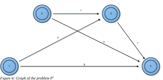
₍_ij)xij≤2

The graph of this problem is shown in Figure 5.

Initialization: Q=P ; z=+∞ ;

• Q=Q ∖ { P }

• RELAX(P):

The solution found is the Shortest Path: [1→2→3→4].

zl=3 ; zu=+∞;

zu>zl and the solution is not feasible because 3>2 then BRANCH is needed.

• BRANCH(P):

P1_{:={ x}

12=0 } // x12=0 means that in P1 the link (1,2) is deleted

P2:={ x12=1 ; x23=0} // link (1,2) is force and link (2,3) is deleted

P3:={ x12=1 ; x23=1; x34=0 } // the links (1,2) and (2,3) are forced, (3,4) is deleted

(36)

Q=Q∪{ P1,_P2,_P3_}

Problem P1 _:

In this problem 1 is the source node and 4 is the destination node. • Q=Q ∖ { P1}

• RELAX(P1_):

The solution found is the Shortest Path: [1→3→4], z_l=4 ; .

Since the path found has a number of link equal to 2, it is a feasible solution to the starting problem.

zu_{=4 ; Since(z}u

<z ) → z=zu_;

(zu

=zl) → The problem is pruned by optimality, no BRANCH needed.

Problem P2_:

This problem can be transformed in an equivalent problem in which 2 is the source node and 4 is the destination node, deleting links (1,2) and (2,3).

• Q=Q ∖ { P2} • RELAX(P2_):

The solution found is the path: [2→4]. Complete solution: [1→2→4].

z_l=1+4 ;

Since the path found has a number of links equal to 2, it is a feasible solution to the starting problem.

(37)

zu_{=5 ; Since (z}u

>z) → z isnot updated

(zl>z) → The problemis pruned by bound , no BRANCH needed.

Problem P3 _:

This problem can be transformed in an equivalent problem in which 3 is the source node and 4 is the destination node, deleting links (1,2) and (2,3).

• Q=Q ∖ { P3_}

• RELAX(P3_):

No possible solution can be found → pruned by infeasibility

At this point Q=∅ and the algorithm ends. The optimal solution to the starting

Figure 8: Graph of the problem P3

(38)

problem P is the solution found in the sub-problem P1 _{: [1→3→4] with cost equal to 4. The}

corresponding Branch and Bound tree is exposed in Figure 9.

3.2 Parallel Branch and Bound

Two basic approaches are known to accelerate the Branch and Bound execution : 1. Node-based strategies that aim to accelerate a particular operation, mainly at the

node level: Computation in parallel of lower or upper bound, branching and so on. 2. Tree-based strategies that aim to build and explore the Branch and Bound tree in

parallel.

Node-based strategies aim to accelerate the execution of the whole algorithm by executing in parallel a particular operation. These operations are mainly associated to the sub- problems, or node, evaluation, bounding, and branching. This class of strategies has also been identified as low-level parallelization, because they do not aim to modify the dimension of the Branch and Bound Tree neither its exploration.

In this thesis the focus is on tree-based strategies because the aim of the project is to create a parallel framework usable with every problem solvable with a Branch and

(39)

Bound approach. Therefore the skeleton is developed with the assumption that the implementation of the functions at the node level, such as the evaluation function of the node and the branch function, are left to the client of the framework, that in case should implement him-selves a node-based strategy to speed-up furthermore the execution of the algorithm.

Tree-based parallelization strategies aim to evaluate more sub-problems at the same time and yield difficulties that have been well identified by G. Authié and C. Roucairol in [13] and [14] :

• Tasks are created dynamically.

• The structure of the tree that has to be explored is not known beforehand. • The assignment of tasks to processors must be done dynamically.

• Algorithmic aspects, such as sharing and balancing the workload or transmitting information between processes, must be taken into account at run time in order to avoid overheads due to load balancing or communication.

Furthermore, parallelism can create tasks that are redundant or unnecessary for the work to be carried out or which degrade performances [19].

The speed-up gained using such strategy would be expected to be equal to the number of problems (tasks) evaluated in parallel p.

For parallel tree-based B&B, one would expect results that show almost linear speed-up, close to p (efficiency close to 100%). Yet, the relative speed-up obtained by a parallel B&B algorithm may sometimes be quite spectacular, >p, while at other times, a total or partial failure (much <p) may be observed. These behavioural anomalies, both positive and negative, may seem surprising at first. They are mainly due to the combination of the speed-up definitions and the properties of the B&B tree where priorities, or the bounding function, may only be recognized a posteriori, once the exploration is completed [15].

Most parallel Branch and Bound algorithms implement some form of tree exploration in parallel. The fundamental idea is that in most applications of interest the size of the Branch and Bound tree grows rapidly to unmanageable proportions. So, if the exploration of the tree is done in parallel, the faster acquisition of knowledge during the search will allow pruning more nodes of the tree. This leads to a lower number of tasks computed causing a possible speed-up greater than p.

(40)

(41)

4 B&B

LOGICAL

IMPLEMENTATION

he thesis project is a parallel Branch and Bound framework developed using FastFlow (section 2.2) that implements the structured parallel programming methodology presented in section 2. The skeleton used to implement the Branch and Bound pattern is the Farm with feedback, this skeleton fits in an efficient and elegant way the needs of divide and conquer problems.

T

(42)

The basic idea behind the execution flow of the skeleton is that in a common divide and conquer approach the algorithm has a set of problems, usually of the same type, to be computed. In this sense the Farm with feedback is an appropriate paradigm to be used to implement this particular computation. In fact the Workers of the Farm support solving more problems of the set in parallel: in each Worker the same function is replicated aimed at solving a single problem of the set and the Workers are obviously executed in parallel by different processing units. A problem solved by one of the Workers is sent back to the Emitter through the feedback channel and at this point the Emitter can evaluate if the problem needs to be further split or not.

This paradigm may used to solve almost every problem presented in section 3.2. In the following list are reported critical problems presented in section 3.2 regarding the parallelization of the Branch and Bound algorithm and how this pattern solves them:

• Tasks are created dynamically.

The Emitter module is responsible of creating new tasks dynamically. After the reception of an evaluated problem from the Workers the Emitter decides if it is necessary to split-up the problem creating new tasks by branching the problem received.

• The structure of the tree that has to be explored is not known beforehand.

The exploration strategy can be decided a priori depending on the type of problem addressed. In case of graphs a good strategy is a breadth-first strategy. To implement this exploration strategy it is sufficient to manage the input channel to the Emitter as a queue.

• The assignment of tasks to processors must be done dynamically.

The assignment of tasks to processors is managed by the skeleton itself. The Emitter scheduling policies determines to which Worker, and then to which processing unit a particular task will be assigned.

• Algorithmic aspects, such as sharing and balancing the workload or transmitting information between processes, must be taken into account at run time in order to avoid overheads due to load balancing or communication.

(43)

Communications between processes are all managed by the skeleton in a transparent manner. The balancing of the workload of the Workers in a Farm can be easy achieved using an on-demand scheduling policies in the Emitter.

The Branch and Bound algorithm is mapped into the Farm skeleton in this way: the Emitter module contains all the state variables of the algorithm like the current best solution and the upper-bound (z in Code 1). The set Q of the pending problems is indirectly contained in the input channel of the Emitter, in this case the input channel is a queue and therefore the exploration strategy of the Branch and Bound tree is a breadth-first strategy. To implement different strategies some modification to the input channel data structure and/or to the Emitter is needed. These cases are not considered in the thesis project and could be cases of interest for further extensions of the framework. The BRANCH method is implemented in the Emitter module, that in case executes it to split a retrieved problem. The choice to implement the BRANCH method inside the Emitter instead that in the Workers derives from the fact that creating new objects in a programming language is often implemented through a request to the Operating System of some memory space. These requests are protected by the Operating System, to avoid the case where the same memory space is assigned to two different requests, using some form of locking mechanism. So also if one can think that the execution of the BRANCH function inside the Workers could be faster, this is not always true because the creation of these objects can't be done completely in parallel: they are executed sequentially by the Operating System. The RELAX and HEURISTIC method are implemented in the Workers. To compute these two methods no state is needed in the Workers and a Farm can be used with no particulars modification to the standard paradigm.

The termination condition is controlled by the Emitter: it keeps track of the number of tasks submitted to and received from the Workers. When the Emitter receives a task from a Worker, it compares the number of submitted tasks with the number of received tasks. If they are equal, and the computed problem received doesn't need to be branched, this means that the set of pending problems is empty and the Workers are idle, so the computation can terminate. When the skeleton terminates the optimal solution is stored inside the Emitter and a dedicated method may be used to retrieve it.

(44)

that more problems are evaluated in parallel inside the Workers; the second comes from the fact that the Emitter executes the BRANCH method in parallel with the executions of the evaluating methods by the Workers.

This structure is a good implementation provided that the Emitter is not a bottleneck, but considering that the BRANCH method has a completion time usually much shorter than the RELAX + HEURISTIC methods and considering also that the BRANCH method commonly provides a high amount of tasks to be scheduled to workers (around 19 in the test application presented in this thesis) it is possible to assume that the Emitter will not be a bottleneck for the parallelism degrees attainable by the current multi-core architectures.

At this point it makes sense to ask ourselves under what conditions the Emitter is not a bottleneck. To answer to this question it is necessary to build up a cost model for the B&B skeleton deriving it from the Farm cost model reported in section 2.1. In the Farm with feedback pattern the Emitter is a bottleneck when its inter-departure Tp-E, that

indicates the mean time between two consecutive departures from the Emitter, is greater than the service time of the Workers divided by the parallelism degree used. In case of the Farm the inter-departure time is equal to the service time of the Emitter Tp −E=TE.

Given that the service time of the Workers is Tw and the service time of the Emitter is TE we

have that the Emitter is a bottleneck for the B&B skeleton if TE/num>Tw/nw where

num is equal to the mean number of sub-problems generated by the BRANCH method and nw is the number of Workers of the skeleton. In the previous formula it is assumed that every time the Emitter serves a new task it splits the task and therefore it will generates num sub-problems that are scheduled to the Workers. The reported formula should be written using, instead of TE, the inter-departure time of the Emitter Tp-E, but considering

that in a real application the pruning of a problem is frequent only near the ends of the execution of the skeleton, we can assume that most of the time the problems will be branched and so T_{p −E}≈T_E/num. Now it is possible to derive the ideal completion time of the skeleton: if in the skeleton there are no bottleneck its completion time is

# tasks×T_W/nw otherwise it is # tasks×T_E/num. From this formulas it can be observed that the expectation is that the completion time of the skeleton scales linearly with the increase of nw until the Emitter becomes a bottleneck. When the Emitter becomes

(45)

a bottleneck the skeleton stops to scale immediately and the completion time from this point forward remains constant.

(46)

(47)

5 C

ODE

I

MPLEMENTATION

: B&B

SKELETON

n this section the developed code for the Branch and Bound skeleton is discussed. The whole skeleton is contained in a single file the B&B.hpp. This file contains more classes that are analysed one by one in the following sections.

I

(48)

5.1.1 Tree node class

The first class encountered scrolling the file is the bb_tree_node class. This class is abstract. A class is abstract when it contains abstract methods that are methods whit no concrete implementation. These methods are declared in the abstract class but their body is empty. This kind of class is used as an interface for the classes that will extend it providing to these classes, by inheritance, all the public/protected fields and methods it contains. To be able to correctly instantiate the classes that extend an abstract class all the abstract methods contained in the abstract class must be overwritten with a concrete implementation. The client of the skeleton have to extend the bb_tree_node abstract class to represent the type of the problems to be solved inside the skeleton. This mechanism is used to ensure that the class that the client has to develop to represent the problems he wants to solve with the B&B skeleton contains all the methods needed to the skeleton to work correctly. In this class all the informations concerning one problem of the Branch and Bound Tree are contained.

class bb_tree_node{ public: bb_tree_node(){ ub=INT_MAX; lb=INT_MIN; solution=NULL; computed=false; unfeasible=false; taskNumber=0; ffalloc=NULL; } […] protected: int ub; int lb; void* solution; bool computed; bool infeasible; int taskNumber; ff_allocator* ffalloc; };

(49)

In the protected fields of this class (Code 5) there iss all the information needed by the algorithm to keep track of the evaluation of the node and additional fields used by the skeleton.

This class has four virtual methods that the client has to implement in the extended class. These methods are:

• virtual bool admissible(): this method returns true if the solution found by the HEURISTIC method is admissible for the starting problem, false otherwise.

• virtual void free(): this method is needed to delete the object through the ff_allocator. The skeleton has been designed in order to support the creation of the objects representing the problems through a ff_allocator. This allocator is provided by the FastFlow library and it is a powerful and fast allocator for parallel applications. In case the client of the skeleton wants to use the ff_allocator to create these object this method must contain all the operations needed to delete the object. This method is called by the skeleton run-time routines instead of the delete instruction in case that the ff_allocator field of these object is not equal to NULL. • virtual void solve(): this method contains the evaluation function that computes

upper-bound and lower-bound for the problem. The RELAX and HEURISTIC methods are implemented here. If the RELAX method gives no solution to the current problem, the infeasible field must be set to true through the dedicated SetUnfeasible() function.

• virtual std::pair<bb_tree_node**,int>* branch(): this method contains the BRANCH method. It returns a pair object where the first element is an array of pointers of type bb_tree_node and the second element is an int indicating the size of the array.

5.1.2 Branch and Bound class

Below the bb_tree_node class there is the ff_bb class that represents the principal implementation of the skeleton.

(50)

private:

//Emitter for MIN Problem class bbEmin: public ff_node {

[…] };

//Emitter for MAX Problem class bbEmax: public ff_node { […]

};

// Worker

class bbW: public ff_node { […] }; ff_farm<>* farm; int nWorker; bbEmin* emitterMin; bbEmax* emitterMax; int problem_type; public:

ff_bb (int nW,bb_tree_node * task,PROBLEM minmax,

const int _nslabs[N_SLABBUFFER]) { farm = new ff_farm<>();

problem_type=minmax; if(problem_type==MIN){

emitterMin = new bbEmin(task,_nslabs); farm->add_emitter(emitterMin);

} else {

emitterMax = new bbEmax(task,_nslabs); farm->add_emitter(emitterMax);

}

std::vector<ff_node*> w;

for(int i=0;i<nW;i++) w.push_back(new bbW()); farm->set_scheduling_ondemand(3); farm->add_workers(w); farm->wrap_around(); } […] }; Code 6: ff_bb class

This object (Code 6) contains a Farm with feedback, Emitter and Worker object for the Farm and an int variable that can be equal to 0, in case of a minimization problem, or

(51)

equal to 1 in case of maximization problem. This int variable is important because the Emitter used to create the Farm is chosen differently depending on that value.

The parameters needed to instantiate the skeletons are: an int nW indicating the number of the Workers for the Farm, a bb_tree_node* task that represents the starting problem to be solved and a PROBLEM minmax that is an int Є [0,1] to specify whether the problem is a minimization or a maximization problem.

Two more things are worth pointing out in the reported Code 6:

• The set_scheduling_ondemand(3) method called over the farm object that is used to set the scheduling policy of the Emitter to an on-demand policy. Two policies are available in FastFlow for the Farm's Emitter: a round-robin policy and an on-demand policy. The first policy schedules tasks to the Workers in a circular way, so each Worker will execute almost the same number of tasks. Even if this policy could seem to balance the Workers load this is not always true, because the tasks assigned to the Workers could have different execution times. The second policy schedules tasks to the Workers depending on the current load. In the FastFlow library the second policy is implemented using a queue for each Worker of size equal to the int passed through the set_scheduling_ondemand() method. The Emitter schedules a task to a Worker only if there is a free spot in its queue. In this way a better load balance is guaranteed among the Workers.

• The wrap_around() method, this also called over the farm object. It is used to tell to the FastFlow library that the Farm created is to be intended as a Farm with feedback.

5.1.3 Emitter class

It is now possible to analyse more in detail the Emitter class, the class here reported is the bbEmin class that is the Emitter class for a minimization problem. The bbEmax class is specular to this one.

(52)

public: bbEmin(void* t){ currentSolution=NULL; number_tasks=1; completedTasks=0; starting_task=(bb_tree_node*) t; if(starting_task->getAllocator()){ starting_task->getAllocator()->registerAllocator(); } starting_task->SetTaskNumber(number_tasks); }

void * svc(void * task) { if (!task) {

return starting_task; }else {

bb_tree_node* t = (bb_tree_node*) task;

if(t->IsUnfeasible()){ //pruned by infeasibility […]

}else if(currentSolution != NULL && t->GetLb() >

currentSolution->GetUb()){ //pruned by Bounds […]

}else if(t->admissible()){ //pruned by optimality […]

}

std::pair<bb_tree_node**,int>* pair = t->branch(); bb_tree_node** newTaskV=pair->first;

int numE=pair->second; for(int i=0; i<numE; i++){ number_tasks++;

bb_tree_node* newTask = newTaskV[i]; newTask->SetTaskNumber(number_tasks); ff_send_out(newTask); } […] } bb_tree_node* getCurrentSolution(){ return currentSolution; } private: int number_tasks; ff_allocator* ffalloc; bb_tree_node* starting_task; int completedTasks; bb_tree_node* currentSolution; };