Synchronization algorithms for modern aeronautical ground communications

Index

Index

Introduction ...1

1. AeroMACS system ...3

1.1 AeroMACS profile: Physical Layer ... 3

2. Mobile WiMAX ...6

2.1 OFDM techinque ... 7

2.2 OFDMA techinque... 12

3. Forward link ...16

3.1 Forward link synchronization... 16

3.1.1 Timing estimation ... 21

3.1.2 Estimation of the fractional frequency offset... 23

3.1.3 Estimation of the integer frequency offset and preamble identification ... 25

4. Reverse link...29

4.1 Reverse link ranging procedures ... 30

4.2 Frame structure in the AeroMACS system ... 32

4.3 Description of the IR procedure ... 34

4.4 Estimation of the synchronization parameters during IR and HO ranging ... 36

5. Simulations...44

5.1 Forward link Analysis... 44

5.1.1 Performance Results ... 47

5.2 Reverse link Analysis ... 55

5.2.1 Performance Results ... 57

Conclusions ...64

Introduction

Introduction

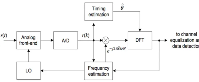
In the design of a digital communication system, the synchronization operation has a considerable importance; through this procedure, starting from the received signal, we can retrieve useful and fundamental information for data detection. In particolar, we can summarize the most important synchronization tasks as [1]:

1) timing synchronization: the goal of this operation is to identify the beginning of each received OFDMA block so as to find the correct position of the DFT window;

2) frequency synchronization: a loss of orthogonality among subcarriers with ensuing limitations of the system performance is caused by a frequency error between the received carrier and the local oscillator used for signal demodulation. Frequency synchronization try to restoring orthogonality by compensating for any frequency offset caused by oscillator inaccuracies or Doppler shifts.

Synchronization is the “focus” of this thesis; it was done in collaboration with the German Aerospace Center (DLR - Deutschen Zentrums für Luft) under the european project called SANDRA [2].

Objective of the SANDRA project is to implement and validate through flight testing a system of integrated aeronautical communications based on an open, a shared set of interfaces and mature standards industry. The high level goals of the project are as follows:

(i) collection and consolidation of existing requirements in different domains and from projects completed or in

progress, possibly extending and enhancing them through the evaluation of regulatory and certification issues;

(ii) establishment of an expanded set of operational scenarios and use cases for the proposed structure;

(iii) defining a system architecture based on a multi-domain.

In SANDRA radio communication systems and antenna will also be analyzed. First of all, a prototype integrated modular radio (Integrated Modular Radio - IMR) with support for multiple radio links will develop, which includes following features: automatic reconfiguration in case of malfunction of a

the service most critical among those running; ability to cross in a continuous manner between the radio links. Regarding in particular the airport connectivity, SANDRA efforts will be concentrated on adaptation and integration of WiMAX into the architecture of the global system through the definition, design and validation of a tecnical profile and an architecture for a telecommunications wide-ranging network based on WiMax. All prototypes developed in SANDRA will be integrated into a final test which aims to validate the concepts developed within the project and to show the benefits of this integrated approach to SANDRA, with regard to the adaptability and reconfigurability, compared to existing systems.

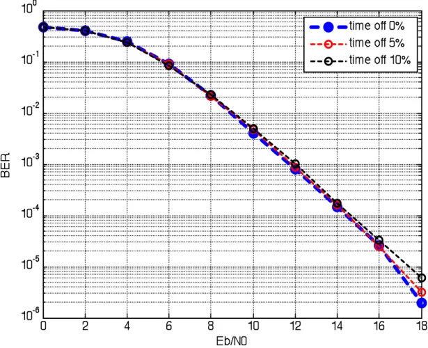
The task covered by the University of Pisa has been to develop and implement the synchronization algorithms for the physical layer of the SANDRA project [3], for an aeronautical communication system for both the forward link and the reverse link. In particular, the thesis’ goal was to evaluate the performance of the system, simulated at DLR using the Java programming language, in terms of BER curves, using the results obtained by the algorithms mentioned above: we studied different scenarios of non-perfect synchronization between the base station (BS) and mobile stations (MS) and for each of them we evaluated the performance of this system using the values of synchronization errors (timing and frequency) arising from the algorithms.

This work is divided into five section: the first is dedicated to discussion of an AeroMACS system and its most important features, while the second is based on brief notes about the WiMAX standard and multiple access techniques OFDM and OFDMA used for AeroMACS system. The third and fourth chapters are devoted to synchronization algorithms developed at the University of Pisa, while the final chapter will describe the results of simulations carried out at DLR.

AeroMACS system

Chapter 1

AeroMACS system

The future airport surface communication system, called AeroMACS, shall be based on the IEEE 802.16 standard, in particular on the "WiMAX Mobile System Profile Specification" [4].

The future Air Traffic Management (ATM) concept shall be based on network centric operations, consequently on information sharing. In order to support such a vision not only a versatile and capable ground based communication network is necessary but also a network which includes the air to ground sub-networks which shall have sufficient capacity and capability. One such air to ground sub-network shall be established for the airport surface intended to be used by departing and arriving aircraft as well as by surface vehicles. This communication system shall be called “Aeronautical Mobile Airport Communications System” (AeroMACS) [5]. AeroMACS shall be based on the IEEE 802.16-2009 standard. A draft profile has been developed and is being evaluated currently in the EU research project SANDRA. The IEEE 802.16-2009 standard specifies the air interface of combined fixed and mobile point to multipoint broadband wireless access systems with the possibility to support different services. The standard specifies the Medium Access Control (MAC) and the Physical (PHY) layer, where the MAC is capable to support multiple PHY specifications applicable to a specific operational environment.

1.1 AeroMACS profile: Physical Layer

The Physical Layer (PHY) of the AeroMACS system shall be based on the OFDMA Physical Layer specification of the IEEE 802.16 standard with a channel bandwidth of 5 MHz. Thereby, the frame length shall be 5 ms. The IEEE 802.16-2009 supports both Time Division Duplexing (TDD) and Frequency Division Duplexing (FDD) modes. However, AeroMACS shall be based on the TDD mode of operation. The reasons which make less complex the use of the TDD option and the reasons for which it is adopte, are the dynamic allocation of forward link and reverse link resources, in order to efficiently support asymmetric forward link / reverse link traffic, and the use of a single

subframe consist of a number of OFDM symbols where a reasonable setting could be to have 29 OFDM symbols for the DL and 18 OFDM symbols for the UL (table 1.1 and table 1.2 show possible data rates with different coding and modulation schemes).

Table 1.1 - Possible FL Data Rates

Table 1.2 - Possible RL Data Rates

The standard supports multiple schemes for dividing the time & frequency resources among users, this may also be called sub-channelization. AeroMACS shall be based on the pseudo-random permutation for frequency diversity. The available spectrum has to be utilized by the resource scheduler through an integer number of FL and RL slots, respectively. A slot is a logical n x m rectangle where n is the number of sub-carriers and m is the number of contiguous OFDM symbols. All slots, no matter which sub-channelization scheme is being used, contain 48 data symbols. Thereby, a FL slot consists of 2 OFDM symbols and 28 subcarriers. As the total usable amount of subcarriers is 420 for the FL, this results in 210 usable FL slots per 5 ms frame in the downlink direction (considering 28 OFDM symbols plus 1 OFDM symbol used for the FL prefix). In contrast a RL slot consists of 3 OFDM symbols and 24 subcarriers. For the uplink direction the total usable amount of subcarriers is 408, consequently there are 102 usable RL slots per 5 ms frame in the uplink direction (assuming 18 OFDM symbols).

Dependent on the coding and modulation scheme different throughput can be achieved. The modulation schemes are QPSK and 16 QAM for both directions

AeroMACS system as well as 64 QAM for the DL direction. 64 QAM is still an option for the UL direction. Dependent on the robustness of the coding scheme different theoretical throughput values can be achieved.

Each 5 ms AeroMACS frame starts with a FL prefix which occupies one entire OFDM symbol. The Frame Control Header (FCH) follows immediately the DL Prefix and contains information about the following FL Map. The FL Map and the RL Map are important management elements which tell the Mobile Stations (MSs) how the upcoming frame is to be used to exchange either data or management information. The mentioned elements of FL prefix, FCH, FL Map, and RL Map appear in each FL subframe. The RL direction needs to schedule ranging opportunities for mobile stations in order to keep synchronized with the base station and in order to request bandwidth if a MS needs to do so. The remaining bandwidth may be used to transmit user data.

Chapter 2

Mobile WiMAX

Mobile WiMAX is a broadband wireless solution that enables convergence of mobile and fixed broadband networks through a common wide area broadband radio access technology and flexible network architecture. The Mobile WiMAX Air Interface adopts Orthogonal Frequency Division Multiple Access (OFDMA) for improved multi-path performance in non-line-of-sight environments [4]. The Mobile Technical Group (MTG) in the WiMAX Forum is developing the Mobile WiMAX system profiles that will define the mandatory and optional features of the IEEE standard that are necessary to build a Mobile WiMAX- compliant air interface that can be certified by the WiMAX Forum. The Mobile WiMAX System Profile enables mobile systems to be configured based on a common base feature set thus ensuring baseline functionality for terminals and base stations that are fully interoperable. Some elements of the base station profiles are specified as optional to provide additional flexibility for deployment based on specific deployment scenarios that may require different configurations that are either capacity-optimized or coverage- optimized.

Mobile WiMAX systems offer scalability in both radio access technology and network architecture, thus providing a great deal of flexibility in network deployment options and service offerings. Some of the salient features supported by Mobile WiMAX are:

a) High Data Rates: the inclusion of MIMO antenna techniques along with flexible sub-channelization schemes, Advanced Coding and Modulation all enable the Mobile WiMAX technology to support peak DL data rates up to 63 Mbps per sector and peak UL data rates up to 28 Mbps per sector in a 10 MHz channel.

b) Quality of Service (QoS): the fundamental premise of the IEEE 802.16 MAC architecture is QoS. It defines Service Flows which can map to DiffServ code points or MPLS flow labels that enable end-to- end IP based QoS. Additionally, sub- channelization and MAP-based signaling schemes provide a flexible mechanism for optimal scheduling of space, frequency and time resources over the air interface on a frame- by-frame basis.

Mobile WiMAX c) Scalability: despite an increasingly globalized economy, spectrum

resources for wireless broadband worldwide are still quite disparate in its allocations. Mobile WiMAX technology therefore, is designed to be able to scale to work in different channelizations from 1.25 to 20 MHz to comply with varied worldwide requirements as efforts proceed to achieve spectrum harmonization in the longer term. This also allows different economies to realize the multi-faceted benefits of the Mobile WiMAX technology for their specific geographic needs such as

providing affordable internet access in rural settings versus enhancing the capacity of mobile broadband access in metro and suburban areas. d) Security: the features provided for Mobile WiMAX security aspects are best in class with EAP-based authentication, AES-CCM-based authenticated encryption, and CMAC and HMAC based control message protection schemes. Support for a diverse set of user

credentials exists including; SIM/USIM cards, Smart Cards, Digital Certificates, and Username/Password schemes based on the relevant EAP methods for the credential type.

e) Mobility: mobile WiMAX supports optimized handover schemes with latencies less than 50 milliseconds to ensure real-time applications such as VoIP perform without service degradation. Flexible key management schemes assure that security is maintained during handover.

2.1 OFDM techinque

At the physical layer of IEEE 802.16e - 2009, as well as in other wireless standards for broadband access in metropolitan area networks or cellular networks recently introduced and future (eg. IEEE 802.20, IEEE 802.11n and 3GPP Long Term Evolution ), is planned for the radio interface to the adoption of OFDMA multiple access technique. This technology builds the core principles of its operation on the reporting scheme multicarrier OFDM (Orthogonal Frequency-Division Multiplexing) combined with technical access (FDMA-Frequency Division Multiple Access). OFDMA is the solution adopted for wireless systems able to provide links to high data-rate, in scenarios in multi-user mobility, where the propagation generally occurs in the absence of direct ray (NLOS - Not Line Of Sight).

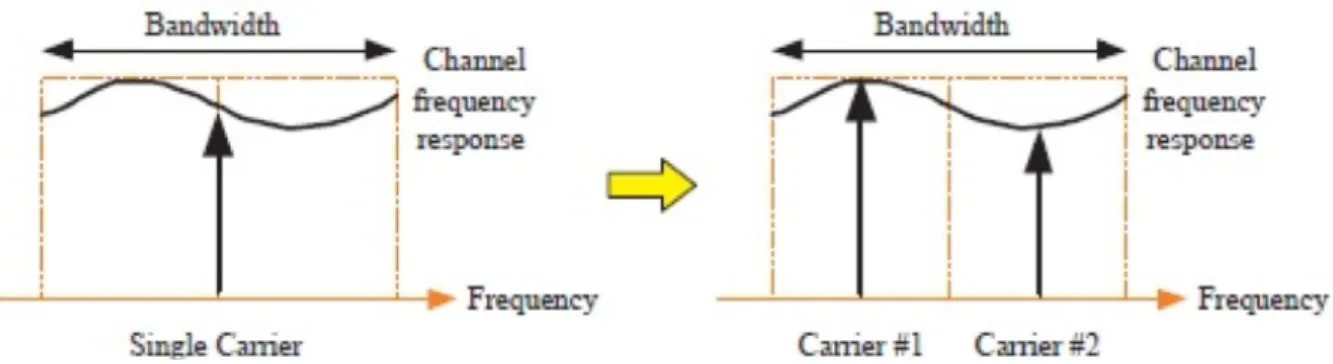
In an environment with multipath propagation, the classification of a channel affected by fading is closely related to the characteristics of the transmitted signal. The information signals pass through frequency-selective channels and,

occurrence of intersymbol interference (ISI - InterSymbol Interference) to the receiver, with a consequent degradation of the quality of the connection. To counter this, instead of using, for example, the classic approach of equalization in the time domain of the single carrier systems, it is preferred to adopt multicarrier techniques.

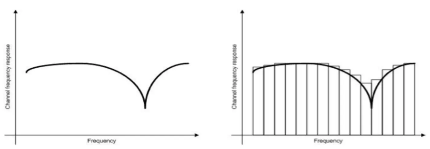
Figure 2.1 - Frequency response of the channel. In a multicarrier system, each subchannel experiences a frequency flat channel.

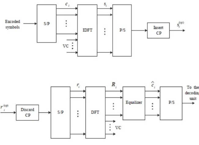
As can be seen from Figure 2.1, in the OFDM technique, the main flow of data at high rate is divided into a number of substreams low rate. Each of them is transmitted on separate subcarriers, orthogonal between them, allowing in this way the "conversion" of the channel selective in frequency in a set of subchannels, partially overlapping, non-selective in frequency (plates). A block diagram of a generic OFDM system is shown in Figure 1.2.

The single stream of encoded symbols is divided into Nu substreams parallel,

each of which, by exploiting the operation of Inverse Discrete Fourier Transform (IDFT) of size N, is modulated on Nu orthogonal carriers

(subcarriers). By appropriately shaping the spectrum of the signal generated in order to prevent possible effects of leakage power in adjacent bands, you can put a zero N - Nu inputs of the IDFT.

Mobile WiMAX

Figura 2.2 - Block diagram of an OFDM system. Above is represented the transmitter, down the receiver.

The corresponding outputs are called virtual subcarriers. The effect of this operation can be appreciated both in the time domain (Figure 2.3), both in the frequency domain (Figure 2.4). In the first case the symbol interval Ts is

increased by a factor of 2 (in general N), in such a way as to be largest (at least by a factor of 10) of the standard deviation of the delays associated with the various paths or the delay value spreads associated with the channel. In the second case, as seen from the spectrum of the output signal to the IDFT, the entire available bandwidth is split into two sub-bands, each of width less than the coherence bandwidth of the channel, so that on each sub-band is experienced a channel flat in frequency.

Figure 2.3 - Illustration of the benefits obtained in the time domain lengthening the symbol interval through the OFDM technique.

Figure 2.4 - Illustration of the benefits obtained in the frequency domain lengthening the symbol interval through the OFDM technique.

As a result of temporal dispersion of the transmitted signal, caused by the finite duration of the impulse response of the channel, it may happen that consecutive OFDM symbols (also called blocks) overlap partially, generating interference interlock (IBI - Interblock Interference). To eliminate this effect it is usual to precede between two adjacent OFDM blocks a guard interval. In particular, for each OFDM block is prepended copy of his last Ng samples of the IDFT, going to be the cyclic prefix. In this way the duration of a single OFDM block is N*T

= N + Ng samples, suitably dimensioning Ng than the duration of the impulse

response of the channel, it is able to eliminate the IBI.

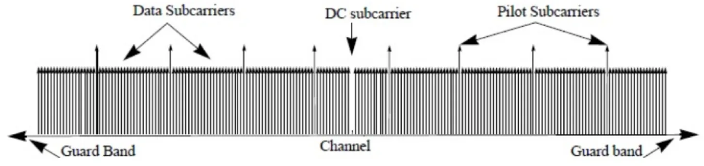
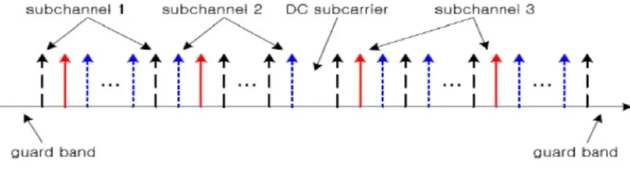
The structure of an OFDM block is represented in the two following figures, in particular, are highlighted in Figure 2.6 the different types of sub-carriers constituting the OFDM symbol.

Mobile WiMAX

Figure 2.5- Structure of an OFDM block.

Figure 2.6 - Structure of an OFDM block. In addition to the subcarriers for the transmission of data and virtual ones (which is also part of the DC subcarrier),

there are the pilotsubcarriers used for the estimation of some parameters. At the receiver, samples of the received signal are divided into segments of length N*T. From this sequence are removed in the first Ng samples (removal of

the cyclic prefix) and the remaining N are sent to the block that performs the discrete Fourier transform (DFT). The outputs corresponding to pass through the block that performs the equalization in the frequency domain (zero-forcing). This last operation (assuming recovery perfect synchronism and in the absence of IBI), is carried out simply by using a bank of multipliers single outlet complex values , in correspondence with each output of the block DFT.

In summary, the OFDM technique is characterized by: • advantages:

1) robustness to small-scale fading. The selectivity in the channel frequency is counteracted by dividing the global spectrum of the

2) high spectral efficiency (compared to FDM), due to the partial overlapping of the spectra of the various subchannels;

3) ability to reduce interference between adjacent OFDM blocks introducing the cyclic prefix;

4) simple design of the system by the adoption of the transformed DFT / IDFT or their version of fast FFT / IFFT;

5) reduction of vulnerability to interfering narrow-band,

6) the possibility of adopting adaptive modulation and coding (ACM Adaptive Coding and Modulation) on each subcarrier.

• disadvantages:

1) high sensitivity to errors in recovering the synchronism of time / frequency;

2) the transmitted signal is characterized by high PAPR (Peak to Average Power Ratio) which involves the use of amplifiers with a large linear zone of operation;

3) the cyclic prefix reduces the spectral efficiency.

2.2 OFDMA techinque

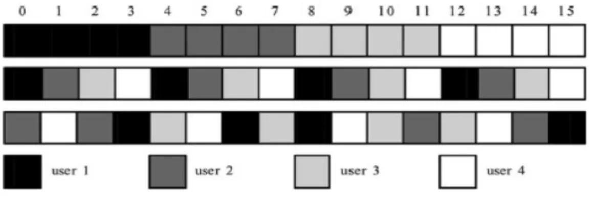
The OFDMA systems are based, as already anticipated, on the OFDM technique [4]. It is therefore to adapt the OFDM system to a multiuser scenario. As shown in Figure 2.7, in the generic OFDMA symbol of the active subcarriers, namely those data and the pilot are divided into clusters (or sub) mutually exclusive. The set of subcarriers, in every time slot, are assigned individually or in groups in a dynamic way (Figure 2.8). The assignment of subcarriers forming one subchannel is carried out according to suitable schemes (CAS - Carrier Assignment Scheme).

Mobile WiMAX

Figura 2.8 - Dynamic assignment of subcarriers.

The patterns of allocation, represented in Figure 2.9, are generally three: • each subchannel is formed by an equal number of adjacent subcarriers. In this way is not exploited frequency diversity provided by a scenario with multipath propagation. If the channel is affected by deep fading may be involved in an excessive number of subcarriers of a given user; • each subchannel is formed by equally spaced subcarriers, in general, with spacing equal to the number of subchannels;

• each subchannel is formed from the best (in terms of SNR) subcarriers currently available for a given user. This is obtained through knowledge of the channel to the receiver / transmitter (CSI - Channel State

Information) using the time division duplexing (TDD - Time Division Duplexing).

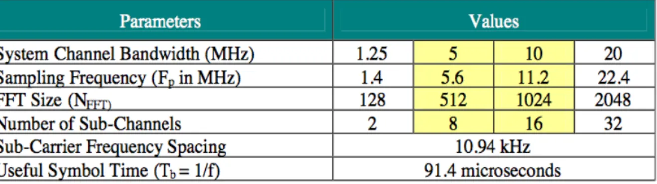
By exploiting the orthogonality between the individual sub-carriers, it is evident how, in the case of perfect recovery of the synchronism, users are mutually protected by multiple access interference (MAI - Multiple Access Interference). OFDMA inherits from OFDM the benefits, and adds the flexibility in allocating resources to users. This flexibility derives from the scalability it offers the S-OFDMA (Scalable S-OFDMA), provided in the IEEE 802.16e - 2009. This is one of the main advantages of OFDMA. In fact, it is able to dynamically manage the bandwidth to be allocated to users, from a minimum of 1.25 MHz to a maximum of 20 MHz. As shown in Table 1.1 this is possible by varying the size of the DFT / IDFT (from 128 to 2048) and consequently the number of the subcarriers, leaving unchanged the spacing (in this case fixed at 10.94 kHz).

Table 1.1 - Parameters of S-OFDMA in the standard IEEE 802.16e.

An OFDMA system inherits from OFDM the problems inherent in the synchronization in time and frequency, being very susceptible to timing errors (timing offset) and frequency error (frequency offset). Synchronization in the time scale is essential to identify the start of the received OFDMA block, in order to identify the exact (or almost) the window for the operation of the DFT. The timing errors are a direct consequence of the onset of IBI consecutive OFDMA symbols. The frequency synchronization is essential for a correct demodulation of the received signal. The frequency offset, namely the difference between the frequency of the received signal and that of the local reference in the receiver, is caused by the Doppler effect and / or instability of the local oscillator. Failure frequency offset compensation affect the orthogonality between subcarriers causing the onset of ICI (intercarrier Interference) and MAI.

The effect of timing errors can be reduced by adjusting the length of the cyclic prefix, however, this value must be chosen suitably (greater than the length of the CIR), for a duration too high would reduce the throughput of the link. In the light of what has been said, in practical applications it is essential to use

Mobile WiMAX The synchronization procedure in a general OFDMA system requires to perform the following steps:

• the mobile station (MS) makes estimates of timing / frequency offset, using signals with appropriate pilot symbols sent by the base station (BS) in the forward link;

• for the transmission on the reverse link the mobile terminal

uses the estimated parameters. The signals arriving at the base station will be affected by the offset due to Doppler shift, propagation delays and errors of estimation in the forward link. In this phase, the BS must be able to discriminate between different users and make estimates of more parameters;

• estimates made by the BS should be used to make the necessary corrections in time and frequency: these estimates may be sent to the MS in the forward link (with reduction of the throughput of the connection time scenarios - variants) or used to make the same BS corrections on the spot, using sophisticated signal processing

Chapter 3

Forward link

The synchronization is a crucial function in a communication system; through it is possible to establish and maintain a communication between two or more terminals. Through the synchronization procedure is possible to extract some parameters from the received signal, for subsequent use as local references of time and frequency. In AeroMACS different algorithms are used for synchronization in FL and RL [3].

In this chapter we made a brief mention on the estimation algorithms of synchronization errors (in both time and frequency domain) developed and implemented at the University of Pisa in the forward link. The results of these algorithms have been used within the Java simulator to calculate the performance of the communication system.

3.1 Forward link synchronization

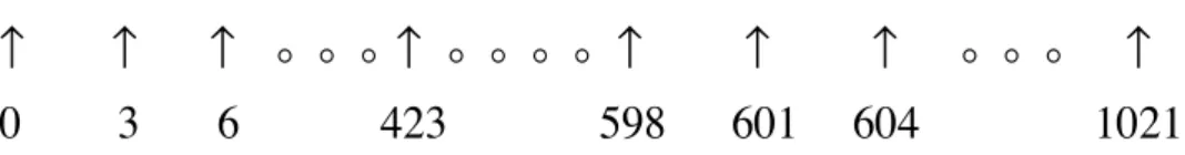
The first task that the MS (Mobile System) must accomplish during the forward link synchronization phase is the detection of training symbol within the stream of received samples. The training symbol is placed at the beginning of each frame (training preamble) and contains N=1024 subcarriers with indices n = 0,1,….., N-1. Out of all available 1024 subcarriers, only a subset of 284 subcarriers are actually modulated by a BPSK pseudonoise (PN) sequence, which is selected among 114 possible choices and univocally identifies the transmitting BS (Base Station). The modulated subcarriers are separeted by a couple of unmodulated (null) subcarriers and there are 86 guard band subcarriers on each side of the signal spectrum. The indices of the modulated subcarriers during the frame preamble are given by

i_m = |η₀ + 3m |_N -142≤m≤141 (3.1)

where η0 ∈ 0,1,2

{

}

is a unknown parameter that designates the preamble carrier-set for identification of the cell sector, while the notation | n |_N denotes the modulo- n operation reducing n to the interval [0, N-1], N is the FFT size.

Forward link Below it is shown the basic structure of the frame preamble assuming η₀ = 0 . As it is seen, we have a first set of modulated subcarriers with indices running from 0 to 423 and belonging to the portion of spectrum placed at the right-hand side of the carrier frequency , while a second set of subcarriers with indices running from 598 to 1021 is placed at the left-hand side of the carrier frequency.

↑ ↑ ↑    ↑     ↑ ↑ ↑    ↑

0 3 6 423 598 601 604 1021

Figure 3.1 - Basic structure of the forward link frame preamble

The training preamble is preceded by a cyclic prefix containing Ng =128 samples. The complex envelope of the transmitted signal is thus given by

sp(t)= A N ap(m)e j 2π (η₀+ 3m)t /T_u m=−142 141

∑

− Tg ≤ t ≤ Tu (3.2)

where a_p = a

{

_p(−142),a_p(−141),...,a_p(141)

}

is the sequence of pilot symbols belonging to the pth preamble (with p = 0,1,……,113 and a_p(m)= ±1) , while A= 2 2 accounts fot the power boosting applied to the pilot tones. Tg and Tu are respectively the guard interval and the ODFM symbol duration without guard interval. It is worth observing that the integer η0 is univocally determined by the preamble index p as specified in the standard.

The samples of sp(t) taken at the instans tk=kTu/N take the form

sp(k)= A N ap(m)e j 2π k(η0+ 3m)/ N m=−142 141

∑

− Ng ≤ k ≤ N − 1 (3.3)

where Ng is the guard interval samples. This expression indicates that sp(t) is the product of a periodic signal with period Tu/3 multiplied by a complex exponential exp j2

{

πη0t / Tu

}

. Unfortunately, such periodicity does not hold true for the corresponding samples sp(k) since N is not a multiple of three. However , we expect tha samples corresponding to the training preamble taken at a distance of N_C = N / 3⎢⎣ ⎥⎦ = N_C = 341 are highly correlated in practice.

We denote by f_Δ the CFO (carrier frequency offset) normalized by the subcarrier spacing. The samples received at the MS and corresponding to the training preamble are thus given by

r(k)

=

A

N

e

j 2π ( f_Δ+η₀)k / N

a

_p

(m)H (i

_m

)e

j 6π mk / N m=−142 141

∑

+ w(k)

_(3.4)

with im being defined in (3.1). The quantities w(k) account for thermal noise and are modeled as statistically independent and complex-valued Gaussian random variables with zero-mean and variance σW

2 _{, while H(i}

m) is the channel frequency

response over the nth subcarrier. Denoting by

h = [h(0), h(1), ……, h(L-1)] the channel impulse response, we have

H (n)

=

h(l)e

− j 2πnl / N

l=0 L−1

∑

0

≤ n ≤ N − 1

_(3.5)

where the energy of h is normalized such that

E H (n)

{

2

}

= 1 (3.6) for n = 0,1 ,……, N-1.

To proceed further, we define the Nc – lag correlation of r(k) as

R_r(N_c)= E r(k + N

{

_c)r*(k)

}

(3.7)

Then, substituting (3.4) into (3.7) and modeling the pilot symbols as statistically independent random variables, we see that during the training preamble it is

R

r

(N

c

)

=

A

2

N

e

j 2π( f_Δ+η0)Nc/ N

e

j 6πmNc/ N m=−142 141

∑

(3.8) or, equivalently,

R

_r

(N

_c

)

= 1.95 * e

j 2π ( fΔ+η0)Nc / N

* e

jπ /N (3.9)

Forward link On the other hand, the samples received at the MS and belonging to an OFDM data symbol are espressed by

r(k)= ej 2π fΔk / N_S

R(k)+ w(k) (3.10)

where sR(k) is the useful component of the received signal, which takes the form

s_R(k)= 1 N c(n)H (n)e j 2πnk /N n=−420 420

∑

(3.11)

In the above expression, the information symbols c(n)

{ }

are modelled as statistically independent random variables with zero-mean and energy

C

₂

= E c(n)

{ }

2 .

Substituting (3.11) into (3.7) provides the NC – lag correlation corresponding to an OFDM data symbol in the form

R

r

(N

c

)

=

C

₂

N

e

j 2πf_ΔNc/ N

e

j 2πnk / N n=−420 420

∑

(3.12)

which can also be written as

R_r(N_c)= 2.1*10−4 * C₂ej 2π fΔNc/ N (3.13)

Comparing the results (3.9) and (3.13) reveals that Rr(Nc) is significantly larger during the training preamble than during an OFDM data symbol. This suggest that | Rr(Nc) | provides uesful information as to whether a training preamble is present or not in the received samples

{ }

r(k) .

Unfortunately, the quantity Rr(Nc) is not available at the receiver due to the presence of the statistical expectation in the right-hand-side of (3.7). To overcome this difficulty, we replace Rr(Nc) by the sample correlation function evalueted over an integration window spanning 2Nc samples. This function is defined as

C(d)= 1 2N_c r * (d+ k)r(d + k + N_c) k=0 2 Nc−1

∑

(3.14)

where d is a time index which slides along in time as the receiver searches for the training preamble. The quantity |C(d)| is then normalized by an estimate of the received energy over the integration window, which is obtained as

P(d)

=

1

2N

_c

r(d

+ k)

2 k=0 2 Nc−1

∑

(3.15)

This provides a metric

M (d)= C(d)

max P(d), P(d

{

+ N_c)

}

(3.16)

which is virtually independent of the instantaneous received power. In order to reduce the implementation complexity, the quantities C(d) and P(d) can be iteratively computed as C(d + 1) = C(d) + 1 2N_c r *_(d+ 2N c)r (d+ 3Nc)− r *_{(d)r (d}+ N c) ⎡⎣ ⎤⎦ (3.17) P(d + 1) = P(d) + 1 2N_c r(d+ 2Nc) 2 − r(d)2 ⎡ ⎣ ⎤⎦ (3.18) for d = 0,1,2,…….., with

C(0)

=

1

2N

_c

r

*

(k)r(k

+ N

_c

)

k=0 2 Nc−1

∑

(3.19) P(0)= 1 2N_c r(k) 2 k=0 2 Nc−1

∑

(3.20)

Substituting (3.4) into (3.5) and computing the expectation yields

E P(d)

{

}

= 284 * A 2 N +σw 2 _{ 2.22 +}σ w 2 (3.21) Bearing in mind (3.9) and (3.21), from (3.16) we see that for d = 0 (which corresponds to the peak of the timing metric) we have

E M (d

{

= 0)

}

 1.95

Forward link

meaning that, at relatively large SNR values, the peak of M(d) is expected to be in the order of 0.85.

In the experiments done, a silent period where nothing is transmitted is followed by a training preamble plus four OFDM data symbols. The propagation channel is taken from the ITU-Vehicular A model and is characterized by six multipath components.

The metric M(d) has a peak in the neighborhood of the training preamble and exhibits a plateau whose duration is approximately equal to the CP (cyclic prefix) length. A synch flag indicating the presence of the training symbol is thus obtained by comparing M(d) with a threshold λ₀. More precisely, assume that M (d₀ − 1) <

λ

₀and M (d₀)>λ₀. Then, a frame detection is declared at d =

d0 , after which the receiver starts a synchronization procedure to acquire timing and frequency information. The threshold must be designed so as to achieve a reasonable trade off between the false alarm probability

P

_fa (i.e., the probability of detecting a frame preamble when it is actually absent) and the misdetection probability

P

_md (i.e., the probability of not detecting a preamble when it is actually present). Clearly, increasing

λ

₀ reduces

P

fa but degrades

the detection capability. A common approach for the threshold design is based on the Neyman-Pearson criterion, according to which

λ

₀is selected so as to achieve a target value of

P

_fa.

3.1.1 Timing estimation

Assume that the metric M(d) overcomes the threshold

λ

₀ at

d

= d

₀. Then, the receiver starts a timing synchronization procedure whose goal is to identify the beginning of each OFDMA block so as to find the correct position of the DFT window. Since the CFO is still unknown in this place, it is desirable that the timing recovery scheme be robust against possibly large frequency offsets. Unfortunately, M(d) cannot provide reliable timing information since the plateau region. A popular approach for timing estimation in multicarrier systems relies on the autocorrelation properties that the cyclic prefix induces on the time domain samples. In practice, the following N – lag autocorrelation function is used as a timing metric

γ (d) = r(d+ k + N)r*(d + k) d₀ + 1 ≤ d ≤

k=0 Ng−1

where NT = N + Ng is the block length (including the CP) espressed in sampling intervals. In practice, is recursively computed as

γ (d + 1) = γ (d) + r(d + N + Ng)r *

(d + Ng)− r(d + N)r *

(d) (3.26) for

d

= d

₀

+ 1,d

₀

+ 2,...,

. Since the CP is just a duplication of the last Ng samples of the ODFM block, we expect that γ (d) exhibits a peak whenever the samples r(d+k) with 0≤ k ≤ Ng − 1 belong to the CP.

In applications where the CP length Ng is relatively small, accurate timing recovery may be difficult to be gained as a consequence of the short integration window employed in (3.25). A possible remedy to this drawback consists of averaging

γ

(d) over a specified number MB of OFDM block. This produces the following modified metric

γ

(d)=

γ

(d+ mNT) m=0

MB−1

∑

(3.27) in which γ (d) is still computed as in (3.25). The timing estimate is eventually found by locating the global maximum of γ (d) over a time interval

I

= d

[

₀

+ 1,d

₀

+ N

_T

]

, i.e.,

d

= argmax

d∈I

γ (d)

{ }

(3.28) It is known that IBI will be present during the payload section of the frame whenever the timing estimate

_d

lies outside the interval Jd= [L - 1,Ng], where L is the CIR length espressed in sampling intervals. Intuitively speaking, the probability of occurrence of IBI can be reduced by shifting the expected value of the timing estimate toward the middle point of

J

_d , which is given by

(L - 1+Ng)/2. This leads the following refined timing estimate

d( f ) = d − E d

{ }

+ (L − 1+ N_g) / 2

(3.29) Extensive simulations indicate that E d

{ }

equals the mean delay associated to the channel response. This parameter is generally unknown at the receiver, but can roughly be approximated by (L-1)/2. Using the result into (3.29), yields the final timing estimate in the form

Forward link

d( f ) = d + N_g / 2 (3.30)

The performance of the timing estimator is assessed in terms of probability of making a timing error, say

P

_f . An error event is declared to occur whenever the estimate _d( f ) gives rise to IBI at the DFT output, which amounts to saying that

d( f ) does not belong to

J

d.

3.1.2 Estimation of the fractional frequency offset

The presence of a carrier frequency offset produces a shift of the received signal in the frequency domain. In multicarrier applications, it is expedient to decompose the frequency error

f

_Δ into an integer part (ICFO), which is multiple of the subcarrier spacing Δf = 1 / T_u , plus a remaining fractional part (FCFO), less than

Δf / 2

in magnitude. This amounts to putting

fΔ =ε +µ (3.31)

where

µ

is integer-valued and represents the ICFO, while ε is the FCFO belonging to the interval (-0.5, +0.5). If not properly compensated, the former results into a shift of the subcarrier indices at the DFT output, while the latter produces ICI and MAI due to a loss of orthogonality among subcarriers. The frequency estimation algorithm provides an estimate of

f

_Δin the form

_f



_Δ

=

ε

 +

µ



(3.32)

where _ε and µ are the estimates of ε and µ respectively. Here, we concentrate on the acquisition of ε, while the problem of estimating the integer offset µ is addressed later.

We begin by considering the timing metric _γ(d) evalueted at the optimum time instant _d given in (3.28). Substituting (3.25) into (3.27) and letting dk.m = d + k + mN_T for notational conciseness, we obtain

γ(d)= MB−1

∑

r(dk.m + N) Ng−1

∑

r*(dk, m) (3.33)

where r(k) are the received samples, which can be espressed as

r(k)= s_R(k)ej 2π fΔk / N + w(k) _(3.34)

In the above equation, w(k) is white Gaussian noise with zero-mean and variance σw

2, while s

R(k) is the useful signal component given in (3.11). To proceed further, we put (3.34) into the equivalent form

r(k)= ej 2π fΔk / N _s

R(k)+

ω

(k)

⎡⎣ ⎤⎦

(3.35)

where ω(k) = w(k)ej 2π f_Δk / N _{has the same statistics of w(k). Then, we assume that} the samples

{

r(d

k, m

); k

= 0,1,..., N

_g

− 1

}

belong to the CP of the mth

OFDMA block. Such a situation occurs with unit probability in the absence of thermal noise and for transmissions over an AWGN channel. In the presence of thermal noise and multipath propagation, it holds true with high probability provided that the timing estimate _d is sufficiently accurate. Hence, neglecting the contribution of IBI for semplicity, we have

r(d

k,m

)

= e

j 2π fΔdk ,m/ N

⎡

s

_R

(d

k,m

)

+

ω(d

k,m

)

⎣⎢

⎤

⎦⎥

(3.36)

r(dk,m + N) = ej 2π fΔ(dk ,m+ N )/N ⎡s_R(dk,m)+

ω

(dk,m + N)

⎣⎢ ⎤⎦⎥ (3.37)

which, combined with (3.33), yields

γ(d)= M_BN_gσ_s2ej 2π fΔ₍₁+η_{) (3.38)} where

σ

s 2 = 1 M_BN_{g m = 0} MB−1

∑

s_R(dk, m) 2 k=0 Ng−1

∑

(3.39) is the received signal energy, and

Forward link η= 1 M_BN_gσ_s2 * m=0 M_B−1

∑

s(dk, m)ω * (dk, m)+ s*(dk, m)ω (dk, m + N) +ω * (dk, m)ω(dk, m + N) ⎡ ⎣⎢ ⎤⎦⎥ k=0 N_g−1

∑

(3.40)

is a disturbance term. Recalling that fΔ = ε + µ , from (3.38) we see that an estimate of the FCFO can be computed as

ε = 1

2π arg

{ }

γ (d) (3.41)

where

arg X

{ }

denotes the principal value of the argument of X.

3.1.3 Estimation of the integer frequency offset

and preamble identification

In the considered AeroMACS profile, the subcarrier spacing is Δf = 10.94 kHz while the carrier frequency is approximately 5 GHz. Assuming an overall oscillator instability of ±2 parts per million (ppm), the maximum frequency offset between the received carrier and the local oscillator frequencies is ±20 kHz, which corresponds to f_Δ = ±1.83 . This means that the ICFO can take values in the set J_µ = ±2,±1,0

{

}

and must be estimated in some manner. Another task that the receiver has to accomplish is the identification of the received training preamble in order to univocally specify the transmitting BS. The training preamble is selected among 114 possible choices and is characterized by a pseudonoise sequence of 284 BPSK symbols modulating one every three subcarriers. The indices i_m(−142 ≤ m ≤ 141) of the modulated subcarriers are espressed in (3.1), where η0 ∈ 0,1,2

{

}

designates the cell sector. In this section a method for jointly estimating the ICFO and transmitted preamble sequence is illustrated.

For this purpose, we use the timing estimate _d( f ) provided in (3.29) in order to select the N samples belonging to the received training preamble, say r(k + d( f ))

with k = 0, 1,….., N-1. Next, we counter-rotate samples _{r(k + d}( f )) at an angular speed

_{2πε / N}

so as to compensate for the FCFO. This produces the frequency-corrected samples

x(k) = r(k + d

( f )

)e− j2π kε /N k = 0,1,..., N − 1 (3.43) which are then fed to the DFT unit, yielding the frequency-domain samples

X(n)= 1 N x(k)e − j2πnk /N k=0 N−1

∑

n= 0,1,..., N − 1 _(3.44)

To proceed further, we consider the situation where the pth training preamble a_p(m);−142 ≤ m ≤ 141

{

}

has been transmitted (with p=0,1,…….,113) and define the following zero-padded sequence

ap

(ZP )_(n)=

{

ap(m) if n= im

0 otherwise (3.45)

with im = η0 + 3m_N for -142≤ m ≤141. Then, assuming ideal FCFO

compensation and recalling that the ICFO results into a shift of the subcarrier indices at the DFT output, we may write

X(n)

= AH(n +

µ)b

_p

(n

+

µ)e

− j2πδd(n+µ)/ N

+ W (n)

(3.46)

A= 2 2

where A is the power boosting factor and bp(n) is the periodic repetition of

ap (ZP )

(n) with period N. Also, W(n) is the contribution of the termal noise while

δ

d is the timing error, which appears as a linear phase shift across the

subcarriers. As anticipated, we aim at jointly estimating the ICFO

µ

∈J

_u and the training index p∈Jp = 0,1,...,113

{

}

. One possible approach consists of looking for the global maximum of the objective function

Φ(µ, p) = Y_p(n;µ)Y_p*(n− 3;µ)

n= 3 N−1

Forward link with respect to (µ, p) ∈J_µ × J_p, where Y_p(n;µ) is the product of the DFT output with the hypothesized shifted sequence

b

_p

(n

+

µ

)

, i.e.,

Y

_p

(n;

µ) = X(n)b

_p

(n

+

µ)

(3.48)

The estimated values of

µ

and p are thus given by µ (µ, p) = argmax

(µ, p)∈J_µ× J_p

Φ(µ, p)

{

}

(3.49)

The use of the metric _Φ(µ, p) can be justified with the following argumets. Substituting (3.46) into (3.47) and neglecting for semplicity the thermal noise contribution, produces

Φ(µ, p) = A4 H (n+ µ)H*(n+µ− 3)d_p(n+µ)d_p(n+µ) n= 3

N−1

∑

2 (3.50)

where d_p(n) is the following differential sequence

d

_p

(n)

= b

_p

(n)b

_p

(n

+ 3)

(3.51) On the other hand, since the channel response is expected to keep approximately constant over three subcarriers, we may put H (n+

µ

− 3) ≈ H(n +

µ

) and rewrite (3.50) as

Φ(

µ

, p) = A

4

H (n

+

µ

)

2

d

p

(n

+

µ

)d

_p

(n

+

µ

)

n= 3

N−1

∑

2 (3.52)

At this stage we apply the Schwartz inequality to show that

Φ(µ, p) ≤ A

4

H (n

+

µ)d

p

(n

+

µ)

2 n= 3

N−1

∑

2 (3.53)

(µ, p) = (µ, p). The above indicates that, in the absence of noise and in case of ideal FCFO compensation, the metric

_Φ(µ

, p)

achieves a global maximum when _(µ, p) = (µ, p), which justifies its use for the joint estimation of µ and p.

Reverse link

Chapter 4

Reverse link

A peculiar feature of the reverse link is that the waveform arriving at the BS is a mixture of signals transmitted by different terminals, each characterized by different timing and frequency errors. The latter cannot be estimated with the same methods employed in the forward link because each user must be separeted from the others before the synchronization process can be started. This makes synchronization in the reverse link much more challenging than in the forward link direction [3]. To alleviate this problem, it is customary to adopt a particolar synchronization policy wherein timing and frequency estimates computed by each terminal during the forward link phase are employed not only to detect the forward link data stream, but also as synchronization references for the reverse link transmission. Due to Doppler shifts and propagation delays, however, the reverse link signals arriving at the BS may still be affected by residual frequency and timing errors. To elaborate on this, let us assume that the BS starts to transmit the lth forward link OFDMA block on the carrier frequency f0 . The block is received by the uth user at t = lTB +τu on the frequency f0 + fD,u , where

τ

u and fD,u are the propagation delay and Doppler shift of the

considered user, respectively. The latter can be espressed as

τu = Δxu c (4.1) and

f

_D,u

=

f

0

υ

u

c

(4.2)

where c= 3 × 108 _{m/s is the speed of light,}

υ

u represents the speed of the uth

terminal and, finally, Δx_u is the distance between the considered terminal and the BS.

As mentioned previously, during the reverse link phase each user aligns its reverse link signal to the BS time and frequency scales by exploiting

particolar, assuming that the forward link synchronization parameters have been perfectly estimated, the reverse link OFDMA blocks are transmitted by the uth user at times iT_B +τ_u (i = 0, 1, 2, …..) on the frequency f0 +fD,u . Due to the

propagation delay and Doppler shift, the BS receives these blocks at iT_B + 2τ_u on the frequency f0 +2fD,u , which results into timing and frequency errors of 2τu

and 2 f_D,u , respectively.

Roughly speaking, the adoption of the illustrated synchronization policy greatly alleviates the reverse link synchronization problem since frequency and timing errors are expected to be much smaller than those encountered in a system wherein reverse link signals are not locked to the forward link transmission. A consequence of this fact is that there is no need of any specific training block in the reverse link synchronization even unnecessary as long as the Doppler shift is adequately smaller than the subcarrier spacing and the duration of the CP is so large to accomodate both the CIR duration and the two-way propagation delay 2τu. In the AeroMACS system, the CP length is either Tg = 5.71µs or

11.42

µ

s.

Assuming a CIR duration T_h = 2.5µs as specified in the ITU-Vehicular channel model and considering the most favourable situation of T_g = 11.42µs, it is found that timing synchronization in the reverse link can be avoided as long as the cell radius is smaller than Rmax = c(Tg – Th )/2 = 1340 m , which reduces to

480 m if T_g = 5.71µs. Since these values seem too stringent for the AeroMACS, we conclude that timing synchronization is mandatory in the reverse link direction. As far as the Doppler shift is concerned, considering a carrier frequency f0 = 5 GHz and recalling that the maximum speed of the

mobile terminals is

υ

_max = 67 km / h , from (4.2) we get 2 fD,u = 620 Hz , which

exceeds the recommended value of 2% of the subcarrier spacing. This means that, in addition to timing adjustement, frequency synchronization is also necessary in the AeroMACS reverse link.

4.1 Reverse link ranging procedures

The reverse link ranging function is used to accomplish some fundamentals tasks, which can be categorized as :

1) initial ranging (IR). This process is performed by any mobile terminal in order to get synchronized to the network before establishing a communication link with the BS;

Reverse link 2) periodic ranging (PR). This process is periodically accomplished by any

active terminal in order to maintain the connection to the network;

3) bandwidth request (BR) ranging. It indicates the procedure by which an active terminal performs bandwidth contention and requests access to the shared spectrum resource;

4) hand-over ranging (HO). It defines the set of operations to manage the hand-over from BS to another.

The fundamental mechanism of ranging involves the mobile terminal transmitting a CDMA code in a specified ranging channel on a randomly selected time slot. As stated in the IEEE 802.16e-2009 standard, the MAC layer at the BS defines a ranging channel as a group of six subchannels. Any subchannel is further separeted into six tiles, with each tile comprising four adjacently positioned subcarriers. The ranging channel is thus composed by 144 subcarriers arranged into 36 tiles. The latter are distributed across the signal spectrum according to a specified permutation formula. A mobile terminal that intends to start a ranging transmission chooses a 144-length pseudo-random binary sequence (PRBS) generated by a linear feedback shift register, which implements the polynomial generator 1+ X1 + X4 + X7 + X15 . After BPSK mapping, the selected code sequence is modulated over the 144 ranging subcarriers and transmitted over the channel. Although the number of available codes is 256, each BS only uses a subgroup of these codes. Initially, the BS will assign more codes for IR as the users within the cell start entering the network. If multiple users are transmitting a ranging signal, they are allowed to collide over the 144 ranging subcarriers.

We denote by bp = [bp(0), bp(1),……, bp(143)] the ranging code selected by a given mobile terminal, where p = 1, 2,….., 256 is an index scanning all 256 available codes. Vector bp is estended to the length N = 1024 by inserting an

appropriate number of zeros. This produces the N – dimensional vector of frequency-domain samples cp = [cp(0), cp(1),……, cp(N-1)] with entries

b

p

(0) if n = i

r

(l)

c

p

(n) =

0 otherwise

(4.3)

where ir(l) is the frequency index of the lth ranging subcarrier. These

signal sp = [sp(0), sp(1),……, sp(N-1)]. The time slot employes for IR and HO

spans two consecutive OFDMA symbols and is obtained by concatenating two copies of sp in the time domain. The resulting vector is then cyclically extended

by inserting a prefix (CPr) and a postfix (CPo) of length Ng . The advantage of this structure is that it avoids any phase discontinuity over the whole ranging slot, with the first copy of sp acting as a sort of long prefix for the second copy. This way, orthogonality among the ranging subcarriers is maintained even in the presence of large timing errors, which only appear as linear phase shifts at the DFT output. In order to improve the code detection capability and the synchronization accuracy, the BS can allocate two adjacent time slots for IR and HO. The time slot employed for PR and BR comprises one single OFDMA symbol. In such a case the ranging signal is obtained by simply appending a cyclic prefix of length Ng to sp . The possibility of using one single copy of sp

instead of two comes from the fact that PR and BR are only performed by terminals that have already been synchronized to the network and, accordingly, they are aligned to the BS time-scale up to an error which is expected to be smaller than the cyclic prefix duration.

4.2 Frame structure in the AeroMACS system

It is useful to illustrate the frame structure employed in the AeroMACS system; a frame consists of two portions, namely the forward link and reverse link subframes. In the horizontal axis there are the forward link and reverse link slots, which consists of two or three OFDMA symbols, respectively, while in the vertical axis there are the logical number of the various subchannels, each containing a set of 24 distinct subcarriers.

Reverse link

Frame structure in the AeroMACS system

The forward link subframe starts with the training preamble followed by the forward link access-protocol (FL-MAP) and reverse link medium-access-protocol (RL-MAP) messages, which provide information about the users’ allocated subchannels and time slots for forward link and reverse link transmissions, respectively. The frame control header (FCH) specifies the information regarding the current frame and its FL-MAP. Next, forward link data are transmitted at allocated subchannels and time slots.

The reverse link subframe is separeted from the forward link packet by a transmit/receive transition gap (TTG). As mentioned previously, any ranging channel is composed by a set of 144 subcarriers arranged into 36 tiles. The remaining portion of the signal bandwidth is employed for reverse link data transmission according to the subchannel allocation specified in the RL-MAP. After a receive/transmit transition gap (RTG), the same structure is repeated for another pair of forward link and reverse link subframes. It is worth observing that, while a training preamble is employed in the forward link direction to facilitate the synchronization process, no preamble is used in the reverse link subframe, where synchronization is achieved during the IR process as outlined in the following subsection.

4.3 Description of the IR procedure

The initial ranging is a contention-based random access process providing network entry and reverse link synchronization. The waveforms transmitted by the mobile terminals arrive at the BS at different time instants depending on their relative position within the radio coverage area and with different Doppler shifts as a consequence of their relative motion. In these circumstances, the reverse link signals will interfere to each other at the BS receiver and the only way to separate them is by means of sophisticated multiuser detection schemes requiring remarkable computational complexity. To overcome this difficulty, the IEEE 802.16e standard specifies a synchronization procedure by which users that are entering the network can adjust their transmission parameters so that reverse link signals arrive at the BS synchronously and with the same power level. The synchronization process is characterized by the sequent steps:

a) each RT that intends to establish a communication link with the BS achieves forward link synchronization. Then, it searches for the Reverse Link Channel Descriptor (RCD) and Forward Link Channel Descriptor (FCD) messages, that are regularly sent by the BS to provide information regarding the physical layer features, such as the adopted modulation type and forward error correcting (FEC) code. The RT also acquires ranging channel information (i.e., available ranging opportunities, ranging subchannels and ranging codes) from the RL-MAP.

b) The synch parameters estimated in the forward link are used as references in the subsequent reverse link phase, during which the RT randomly chooses an available ranging contention slot and sends a ranging request packet (RNG-REQ) to the BS in order to notify the request of network entry. The packet consists of one or two ranging codes, depending on whether the ranging signal is allowed to span two or four OFDMA symbols. If multiple RTs transmit their ranging signal simultaneously, they are allowed to collide on the same ranging channel.

c) As a result of different locations and mobility, ranging signals transmitted by different RTs arrive at the BS with thier specific transmission time delay and Doppler shift. After separating colliding codes, the BS extracts the corresponding timing, frequency and power information, and allocates forward link and reverse link resources to the identified codes for further transmission. For each detected code, the BS checks whether the estimated values of timing, frequency and power are adequately close to the specified requirements. In the affermative case, the BS performs step e), otherwise it proceeds to step d).

Reverse link d) The BS has no way of knowing which MT sent the RNG-REQ. Therefore,

upon succesfully detecting a CDMA code, it transmits a ranging responde packet (RNG-RSP) with “continue” status, indicating the detected code and the corresponding ranging opportunity (OFDMA symbol number and subchannel number) where it has been identified. It also provides instructions for timing, frequency and power adjustement so that the reverse link signal of the corresponding RT can arrive at the BS at the designated time and with the appropriate frequency and power level. Then, the RT shall continue the ranging process as done on the first entry by choosing a new code from the initial ranging domain, which is sent on the periodic ranging region with updated synch parameters. If the RT does not receive any responde message from the BS, after a specified time it performs another ranging attempt using a new randomly selected ranging code and with a higher power level.

e) The BS transmits a RNG-RSP with “success” notification so as to inform the RT that the IR procedure has been successfully completed. Then, the RT sends its identification information to the BS, which eventually performs authorization and registration of the new user.

The above discussion indicates that the main functions of the BS during the IR process may be classified as multiuser code identification and multiuser estimation of timing, frequency and power.

We will assume that users other than those performing IR are already synchronized to the BS and, accordingly, they do not generate inteference over the ranging channel. This is a reasonable assumption as achieving synchronization to the BS is mandatory before a given terminal can start its data transmission. On the other hand, ranging signals arriving at the BS are still unsynchronized and, in consequence, they will interfere with the data subchannels. Since this situation is unavoidable, each RT is required to start the IR process with a relatively low power so as to limit the interference with the reverse link data signals as much as possible. If a RT fails to get a response message from the BS, it retransmits its ranging signal in a next available time-slot by incrementally increasing the power level until a response is detected. If the maximum power level is reached and still the RT cannot get a response from the BS, the RT repeats the IR process starting again from the minimum power level. In order to minimize the probability of a collision, the time between two successive ranging attempts is typically randomized in the basis of some specified contention resolution method. The approach adopted in the IEEE 802.16e standard relies on the truncated binary exponential backoff (BEB) algorithm, which can be summarized as follows. Before each ranging attempt, the RT uniformly chooses an integer number from the interval [0, W -1], where