An attempt of the Variscan (Hercynian) basement top reconstruction in some sectors of Italy (on land and offshore in the Adriatic Sea)

(1)

An attempt of the Variscan

(Hercynian) basement top

reconstruction in some sectors of

Italy (on land and offshore in the

Adriatic Sea)

Eugenio Trumpy

Department of Earth Sciences Pisa University

A thesis submitted for the degree of Earth Sciences Doctor (PhD)

(2)

1. Reviewer: Prof. F.M. Elter

2. Reviewer: Prof. M. Pipan

Day of the defense:

(3)

Abstract

The last decade’s growth in technology has brought a major development in computational tools, hardware and software, in the field of earth sciences. The work is the result of synergistic activity between the classical regional geology and the analytical processing methods typical of the geostatistics and geological. The main objective was to reconstruct, on the basis of avail-able data, the Variscan top surface, preceding the pre-Alpine sedimentary cycle (Upper Carboniferous - Permian) and the Alpine properly Mesozoic and Tertiary, over an area covering the italian peninsula and the Adriatic Sea. The integration of surface geology with the underground information and the interpreted seismic reflection data has been the base of the compu-tation, first on small scale using geostatistical tools and then on large scale with the development of a detailed 3D geologic volume model detail in a geothermal area of Tuscany. The geostatistical processing has produced a series of maps on a national scale relating to the depth of the investigated surface. Available crustal seismic profile were used to this aim, and the first reconstruction was done in the time domain. Then, the velocity was calibrated using subsurface information from deep well stratigraphy, and the obtained model were used to obtain the surface depth values.

The 3D geological model constructed on the basis of subsurface data, wide-spread in the Tuscan geothermal provinces, has instead highlighted the volumes and geometric relationships between the various rocks taken into account, and defined in detail the shape of the Variscan surface. The re-sulting degree of confidence in the results is uneven, depending on the data distribution of subsurface information from wells. However, this method has been readily replicable, and produce easy and fast updated result when new data were introduced. The obtained tools are powerful in supporting activities to study and identify natural deep georesources.

(4)

List of Figures

2.1 Relationship between very close samples correlated, 1, distant low cor-relation, 2, distant and not correlated, 3, with the point considered (A) and relationship between distance and correlation, or autocorrelation

(B), from (164) . . . 15

2.2 Z(x) values along a particular direction of space (A) and subdivision of the total variability into two components (B), from (164) . . . 16

2.3 Semivariogram function example, from (164) . . . 17

2.4 Example of variogram models, (164) . . . 19

2.5 Irregular sampling, from (164) . . . 21

2.6 Example of a map of the variogram, from (164) . . . 22

3.1 Western Mediterranean paleotectonic maps, from (145). Brown area: continental crust. Green area: oceanic crust. The red arrows are the regional trascurrent faults (in A and B), the red line with red triangles indicates subduction lineaments. The double red arrows indicate the opening of the provential-ligurian basin (C) and the Tyrrhenian basin (D) 31 3.2 Lateral extrusion model applied to the Apennine Chain, the frame of convergence between Africa and Eurasia at Pliocene, from (21) . . . 32

(7)

LIST OF FIGURES

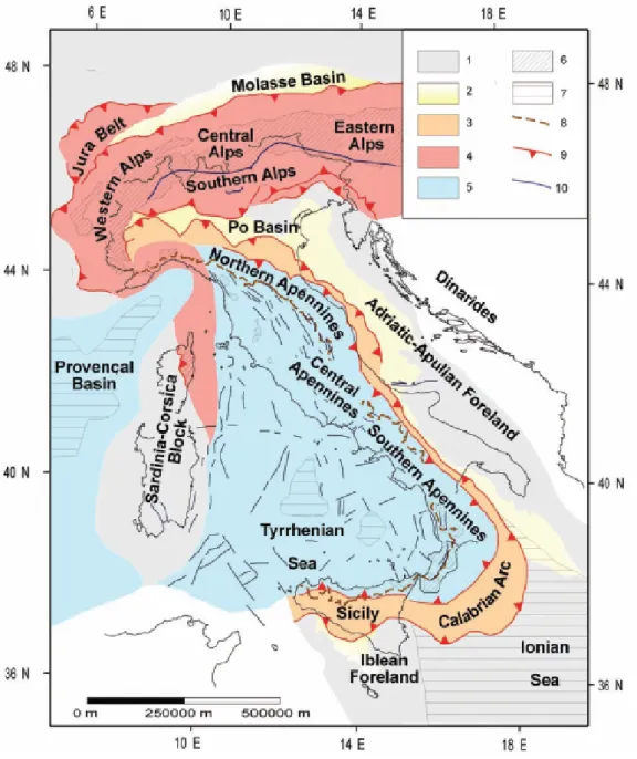
3.3 Synthetic tectonic map of Italy and surrounding seas; 1) Foreland ar-eas; 2) foredeep deposits (delimited by the 1000 m isobath); 3) domains characterized by a compressional tectonic regime in the Apennines; 4) thrust belt units accreted during the Alpine orogenesis in the Alps and in Corsica; 5) areas affected by extensional tectonics: these areas can be considered as a back-arc basin system developed in response to the eastward roll-back of the west-directed Apenninic subduction; 6) out-crops of crystalline basement (including metamorphic alpine units); 7) regions characterised by oceanic crust: an oceanic crust of new formation has been recognised in the Provenal Basin (Miocene in age) and in the Tyrrhenian Sea (Plio-Pleistocene in age) while an old mesozoic oceanic crust can been inferred for the Ionian Basin; 8) Apenninic water divide;

9) main thrusts; 10) faults (from (182)) . . . 34

3.4 Map of magnetic basement from (201) . . . 41

3.5 Map of gravimetric basement from (201) . . . 42

3.6 Depth to basement (km) from (190), the number are the references to the used data, see (190) . . . 43

3.7 Cross-sections illustrating two different interpretations of the same data from a hypothetical carbonate ridge flanked by flysch. In (a) uplift and folding have resulted from thin-skinned thrusting and duplication of the stratigraphy at depth. In contrast, uplift in interpretation in (b) is due to reactivation of a pre-existing extensional fault that originally hosted an increased thickness of sediment. Note that the shortening in (b) is almost four times less compared to (a), see (194) . . . 45

3.8 Geological map: reclassified legend . . . 49

3.9 Tuscan region - Geological map reclassified . . . 50

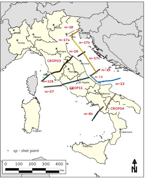
4.1 The base map, are shown the location of the shot point belongs to each interpreted seismic CROP profile used (CROP seismic interpreted cross-section attached to ??) . . . 53

4.2 Example of measurement activity . . . 55

4.3 The map of the geologic domains . . . 58

(8)

LIST OF FIGURES

4.5 The schematic geologic cross-section, are shown the domains ant the main deep thrusts considered. ONA is Outer Northern Apennines. Not

in scale . . . 60

4.6 Deep wells localization . . . 62

4.7 Avampaese deep wells . . . 63

4.8 A core slice from Foresta Umbra 1 wells, anhydrites from 4233 . . . 65

4.9 Onshore deep wells . . . 67

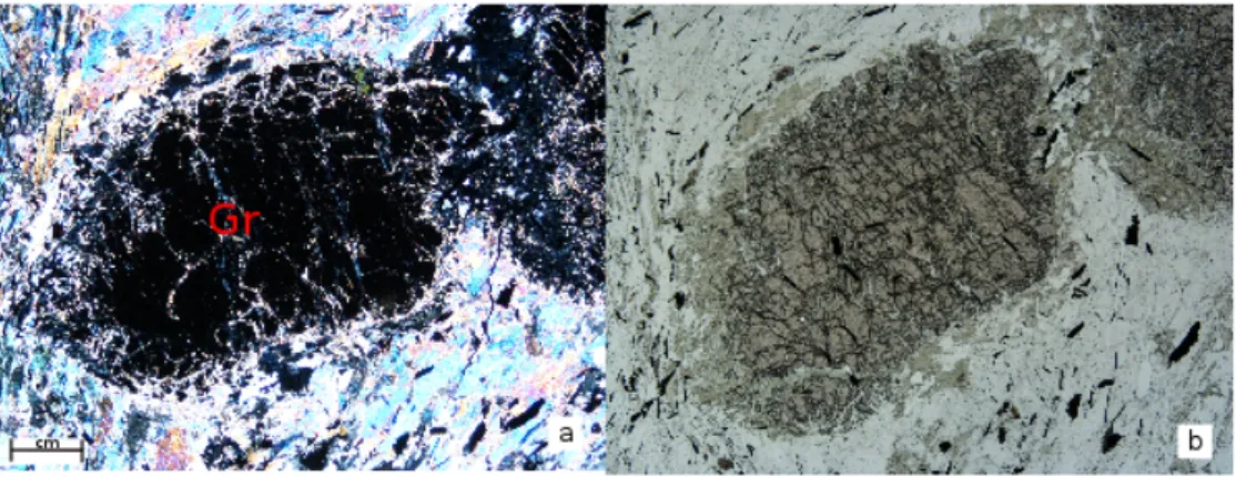
4.10 A clastic detritic thin section of a sample taken from Perugia 2 well at about 1400 m depth. Correlated with quarzitic formation of the Ver-rucano group. With the red mark the S1 cleavage deformation - Thin section by courtesy G. Gianelli (CNR - IIRG), 1980 . . . 68

4.11 A layered micaceous schist thin section from Perugia 2 at about 1447 m depth. Are clearly recognizable the S1 and S2 schistosity plane, the S1 (light red line) is present in the microlithons and is trasposed by S2 foliation (red line). With the dashed yellow line is marked the crenulation S3 - Thin section by courtesy G. Gianelli (CNR - IIRG), 1980 . . . 68

4.12 A more layered micaceous schist thin section from Perugia 2 at about 1447 m depth. Also in this case are evident 3 plane of schistosity, the relicts S1 (light red line) in the microlithons, separated by the main S2 foliation (red line) and finally the structure is crenulated by the S3 (dashed yellow line) - Thin section by courtesy G. Gianelli (CNR - IIRG), 1980 . . . 69

4.13 A micaschist/paragneiss sample from Pontremoli 1 well, from 3422 mm depth. a) Nx pic representing a micaceous part with two deformation, the relict S1 bounded by S2. b) Nα pic, same sample . . . 70

4.14 A micaschist sample from Pontremoli 1 well, from 3520 mm depth. a) Nx pic representing a garnet, about 4,8 mm in length. b) Nα pic, same sample . . . 71

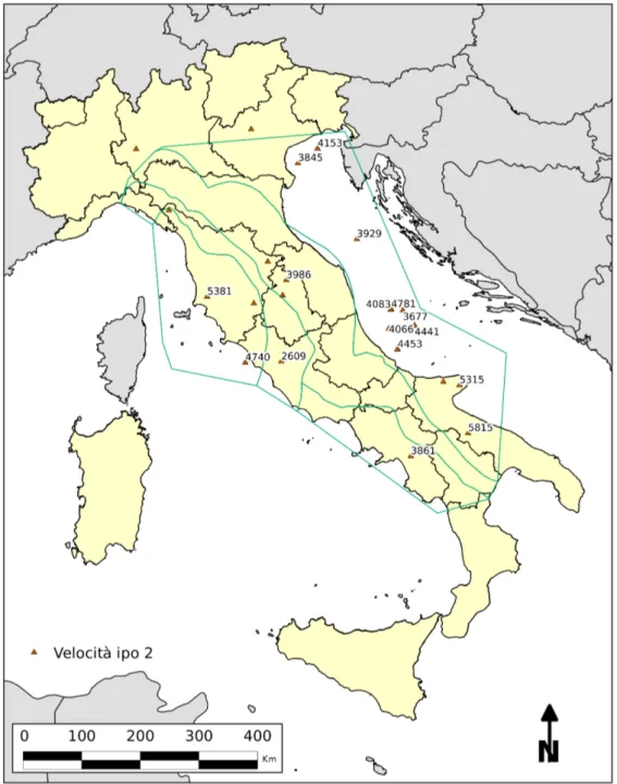
4.15 The map represents the verticals velocity calculated with hypothesis 2 methods . . . 79

(9)

LIST OF FIGURES

4.17 The map represents the verticals velocity calculated with hypothesis 7

methods . . . 81

4.19 The resulting Voronoi polygon for the Avampaese domain are shown . . 83

4.20 Histogram in frequencies classes of the Bas 1 variable . . . 86

4.21 The denisty curve of the Bas 1 variable . . . 86

4.22 Here there are represented some outputs of R software obtained in the study of the variogram for the variable studied. a) is the variogram orig-inally calculated, b) shows the map of the variance of the variogram, c) the variogram calculated according to the direction of anisotropy us-ing a model 135 automatic spherical, d) with the best variogram model calculated with the cross-validation procedure that is proved to be an exponential model automatically . . . 88

4.23 Here there are represented the cross-validation residuals distribution. a) exponential model manually fitted. b) exponential model automatically fitted . . . 89

4.24 The rusulting Universal Kriging map for Avampaese domain. a) The time map of the variable Bas 1, represent the thickness in TWT in mil-limeter (mm), where 10 mm = 1 second (s). b) The variance map of the variable Bas 1 . . . 90

4.25 Histogram in frequencies classes of the Bas 1 variable . . . 92

4.26 The denisty curve of the Bas 1 variable . . . 92

4.27 The variogram of the Bas 1 variable . . . 93

4.28 The map of the TWT in the outer Apennines domain obteined with v.surf.rst module of GRASS GIS . . . 94

4.29 The resulting RST map. The time map of the variable Bas 1, represent the thickness in TWT in millimeter (mm), where 10 mm = 1 second (s). a) Inner northern Apennines time map b) Outer northern Apennines time map c) Inner southern Apennines . . . 96

4.30 The final map of the TWT depth for the whole area. This surface rep-resent the top of the Variscan basement in the time domain . . . 97

(10)

LIST OF FIGURES

4.31 Schematic example of overlapping raster maps. a) Overlaying b) Vertical cells involvement . . . 98 4.32 An example of raster map calculation, in this case the difference between

the rainfall99 and rainfall 98 is calculated . . . 98 4.33 The top of the Variscan basement calculated considering V ipo1 . . . . 99 4.34 The top of the Variscan basement calculated considering V ipo2 . . . . 100 4.35 The top of the Variscan basement calculated considering V ipo2 and

its spatial distribution into the Avampaese domain according with the Voronoi polygon . . . 100 4.36 The top of the Variscan basement calculated considering V ipo6 . . . . 101 4.37 The top of the Variscan basement calculated considering V ipo6 and

its spatial distribution into the Avampaese domain according with the Voronoi polygon . . . 103 4.42 The synthetic Variscan basement map for the Italian area, calculated

considering V ipo7 . . . 107 4.43 The synthetic Variscan basement map for the Italian area, calculated

considering V ipo7 and its spatial distribution into the Avampaese do-main according with the Voronoi polygon . . . 108

(11)

LIST OF FIGURES

5.1 Principle in 2-Dimensions of the geostatistical interpolation using the potential field method. (a) A geological body observed by the locations of its contacts and dip measurements, the red and blue point represent equipotential interface that will be interpolated by co-kriging method. (b) The geological body modelled by potential field method. Interfaces are drawn as isovalues of the interpolated scalar field. Isolines for a 2d scalar field Isosurfaces for a 3d scalar field, from (38) . . . 111 5.2 Multipotential fields allow Onlap and Erod relations between interfaces.

(a) Interpolated formation 1 (basement). Data for potential field of formation 2 in black. (b) Formation 2 interpolated with Onlap relation. Data for potential field of formation 3 in light grey. (c) Formation 3 interpolated with Erod relation, from (38) . . . 112 5.3 3D geological modelling methodology, from (38) . . . 113 5.4 Tectonostratigraphic units in the Larderello geothermal area, reconstructed

on the basis of field and borehole data (not to scale). Symbols: MPQMiocene, Pliocene and Quaternary sediments; Tuscan Nappe (TN): TN2Early MioceneRhaetian sequence; TN1 Late Triassic evaporites; MonticianoRoc-castrada Unit (MRU): MRU3MesozoicPalaeozoic Group, made up of dolostones and limestones (Late Triassic), quartz metaconglomerates, quartzites and phyllites (Verrucano Group, MiddleEarly Triassic),

sand-stones, phyllites (Middle Late CarboniferousEarly Permian); MRU2PhylliticQuartzitic Group; MRU1Paleozoic Micaschist Group; GCGneiss Complex; MR

magmatic intrusions, from (35) . . . 114 5.5 Geological section across the Larderello - Travale geothermal area, from

(30) . . . 116 5.6 Geological-structural cross-section of the Sassa-Guardistallo Basin, from

(57) . . . 116 5.7 Base map of the modelled area . . . 117 5.8 Stratigraphic pile created . . . 118 5.9 Some steps in building model: (a) The base map with the boreholes and

cross-section location. (b) inserting the geologic constrains, interfaces data point and polarities of the geological structures . . . 119 5.10 Section 3 . . . 121

(12)

LIST OF FIGURES

5.11 Section 2 . . . 121

5.12 Section 13 . . . 122

5.13 Section 12 . . . 122

5.14 Geological map, from (118) . . . 123

5.15 Geological map resulting from 3D Geomodeller . . . 124

5.16 Resulting surface in 3D Geomodeller view . . . 124

5.17 Resulting surface in 3D Geomodeller view, with the boreholes used . . . 125

5.18 Resulting 3D Geomodeller geologic block diagram . . . 125

5.19 Geological map, the red line are the inserted faults, from (118) . . . 126

5.20 Section 1 . . . 126

5.21 Section 16 . . . 127

5.22 Section 13 . . . 127

5.23 Section 6 . . . 128

5.24 3D view of the topological surface, the wells and the faults . . . 129

5.25 Resulting 3D Geomodeller bottom surface of the geological layers with boreholes and faults surfaces . . . 129

5.26 Resulting 3D Geomodeller fence diagram, some geological cross-section with the faults surfaces . . . 130

(13)

List of Tables

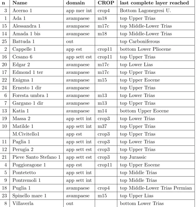
4.1 Used wells, geologic domain membership, CROP profile on which the well is projected, last complete layer reached . . . 73 4.2 Litho-stratigraphic information of the Amanda 1 bis well, in Trieste gulf

located . . . 74 4.3 This is the velocity table proposed by (87) for the Adriatic sea. We used

these values for the Avamapese domain . . . 75 4.4 This is the velocity table proposed by (12) for the northern Apennines

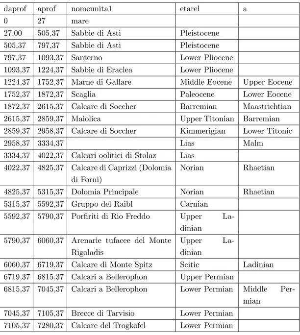
chain. We used these values for the AE, ASI, ASE domains . . . 75 4.5 In the table are shown the seismo-facies time intervals, the thicknessand

depth of each layer . . . 77 4.6 Velocity table, values assigned for each geological domain . . . 78 4.7 Interpolation method . . . 84 4.8 Basics statistic for the varible Bas 1. Bas 1 represents the twt

(multi-plied for 10) to reach the Variscan basement top surface and the return in the surface . . . 85 4.9 Cross-validation results . . . 87 4.10 Basics statistic for the varible Bas 1. Bas 1 represents the twt

(multi-plied for 10) to reach the Variscan basement top surface and the return in the surface . . . 91

(14)

1

Introduction

Understanding the processes that regulate the functioning of the Earth system in a geological sense, is critical to the development of human activities, both in terms of view resource exploitation, and from that of protection and prevention of natural events that may interfere more or less heavily with human life. The knowledge of the struc-ture of the Earth and its evolution over time is crucial to predict the fustruc-ture assets. Since the understanding geological evolution of how an area evolves, like all scientific disciplines, with analytical techniques incessant improving, also including reference to the commonly used models are subject to change if new important data are product that call into question previous interpretations. The project has the goal of achieving a reconstruction of the top surface of the Variscan basement, or older, in the Italian region.

Chapter 2 describes the used softwares, applied geostatistical methods while data were retrieved, processed and integrated to achieve the project objective. Four software were mainly used: two of them for data analysis in a GIS environment, one for a statis-tical and geostatistics analysis and the last for the processing of the three-dimensional geological models. The GIS software used were QuantumGIS and GRASS GIS, both open source and fully integrated with each other, the first used to create the output cartographic representations, while the latter to make some geospatial analysis. The statistical software R, which also lends itself to a seamless integration with GRASS, was used to perform spatial interpolation with the kriging method. Finally, the use of the software 3DGeomodeller, allowed the development of a local geologic model in three dimensions. The used interpolation procedures were mainly of two types, deterministic

(15)

and stochastic. The deterministic method was the Regularized Spline with Tension (RST), developed with GRASS GIS, while the stochastic was kriging, calculated with R. the TWT map and the velocity maps are combined with each other using the equa-tion The used geological data are divided into surface data, geological maps found and used and those underground, made available by National Geothermal Database of the Institute of Geosciences and Earth Resources, CNR, Pisa. The geophysical data refer to the gravimetric data provided by Ispra, Italy, some magnetic maps and mainly the interpreted seismic profiles of the CROP Project, (87).

Chapter 3 describes the geological context in which the Italian area is, at first putting it into the evolutionary framework that characterized the Italian peninsula and in particular the Apennines orogen, then describing the main Variscan outcrops present. The Sardinian-Corsian Variscan outcrops, the Peloritani Calabro massive, the basement known in Tuscany in the Apuan area, in the southern Tuscany and finally with the sequences of the Carnic Alps are describes. This chapter also shows a brief summary of work on the issues addressed by various authors over relative time to the stratigraphic and structural aspects of the Variscan or older basement in Italy. Finally, it describes the geological map taken as the working basic and what considerations were made while preparing the revised geological map functional to the purposes of the project. The Geological Map of Italy at the scale 1:1,000,000 was reclassified by considering the chrono-stratigraphic factors perceived in the original legend, then groups of rock complexes were identified and defined and after a reclassification a geological map where they were distinguished: the Cambro-Carboniferous basement in the sensu stricto, the coverage of the underlying discordant stands in solidarity with it, defined as integument (Permo-Triassic Carboniferous), finally in the Alps the Pennidic complex, including the internal crystalline massifs, Alpine metamorphic complex with original partial coverage and with their fictitious covers. Among vulcanitic complex differed those of Variscan from those tertiary.

The methodological process applied to the data to attempt to reconstruct the top surface of the Variscan basement is described in Chapter 4. Based on acquired data from seismic profiles of the CROP Project and considerations made possible by the geological surface evidence, the subsurface data taken into account and ultimately also by geophysical data, i defined a structural setting model for the Apennines chain in the studied area characterized by some regional overlap that allowed the superimposition of

(16)

crustal portions. In this context, the available data were separately processed for each geologically homogeneous area with diverse interpolative methods for the chain and foreland domains. In particular, we developed a map of TWT with the RST method in the domains of the Apennines chain, while it is achieved through the method of kriging in foreland domain. Then, using the calculation of raster maps (MapAlgebra) maps of the depth, objective of the project were developed. A key step was the study of the velocity field, is necessary to define the velocity maps to be used in MapAlgebra to obtain depth maps. The study of the velocity field was carried out on some vertical localized in the CROP seismic profile in correspondence to some deep surveys. The MapAlgebra was made using the GRASS GIS software. The limiting aspects of the used system and the positive and beneficial of this similar procedure were evaluated.

The 3D geological modeling was discussed in Chapter 5. With the software 3DGe-omodeller a volume model in the geothermal area of Larderello was developed. The choice of the study area fell on the Tuscan geothermal province because, over time, it was intensively drilled for geothermal purposes, the wealth of subsurface data were essential in the selection of this study area. The modeling process was interactive, once data were prepared and imported into the software. We first create a simplified model without considering the possible dislocations caused by faults, and then we attempted the reconstruction by including these structural features. The result is a volume model, where you can create endless horizontal and vertical sections, and obtain volumetric nu-meric values of the geologic complex considered. Some limiting aspects of this method are then discussed.

The final chapter 6 presents a brief discussion of the used data and the method-ologies, the main results obtained and the limiting aspects of the methods used in this work.

(17)

2

The experimental geologic

modeling

2.1 Used software

The aims of this project is to define the top of the Variscan basement in the Italian peninsula area using some modern technologies provided by the informatic tools. The multidisciplinary nature of the geological modeling, gives us the possibility to use geo-logical data from various sources and integrate each other, employing model software, and it opens wide possibilities to reinterpret the existent data and developing new hy-pothesis. In this work, even if the obtained geologic aspects play an important role, also the technological point of view and the methodology used today becomes very impor-tant, in fact, they allow us to obtain the result quickly, (by using a defined procedure) and newly added data reach immediately a more accurate output. Another focal point is the possibility to know, with a certain confidence level, the value of the modeled item where the observation data are unknown in order to have a more exhaustive view of the modeled process.

The main idea was to make use of the open source softwares, because it allows high interoperability and integration. This is a good skill as it allows software to do the job for which it was designed. Here below the most important softwares used and their principles skills are described:

• GRASS GIS for all the spatial analysis

(18)

2.1 Used software

• PostgreSQL with PostGIS to manage the databases • R-project for all statistic and geostatistic tools

To obtain a 3D geologic model it was also used a non open source software named 3D Geomodeller developed and distributed by Intrepid geophysics, (an Australian geo-physics software house) which sells a convenient academic license too. In the next section the most important used softwares characteristics are described.

2.1.1 Grass GIS

According to Burrough (1986) a Geographical Information System is composed by a series of softwares to acquire, store, select, transform and visualize spatial data from the real world. It involves a computer system and allows to produce, manage, analyze spatial data relating to each geographic elements one or more alphanumeric descrip-tions. A GIS could be seen as a Spatial Data Base Management System (SDBMS). To represent the data in a computer system is necessary to formalize a flexible rep-resentative model that fits the real phenomena. In the GIS there are three types of information:

• geometric information: related with the cartographic point of view of the ob-jects represented; like the shape (point, line, polygon), the dimension and the geographycal location;

• topologic: referring to the mutual relations between the objects (connection, ad-jacency, inclusion, ecc..)

• attribute: numerical data, textual data, ecc.., related to each object and managed with a Relational Data Base Management System (RDBMS)

Another fundamental aspect of the GIS is the geometric one, because it saves the data position by using a reference system which defines the object’s geographic position. The GIS manages at the same time the data coming out from different reference systems (e.i. Gauss-Boaga/Roma40, UTM/WGS84, latitude-longitude). In spite of the paper maps, the scale, in a GIS is a parameter of the acquisition data accuracy and not a visualization outset. The real world could be described in a Geographical Information

(19)

2.1 Used software

are made by simple elements as points, lines and polygons coded and stored on the base of their coordinates. A point is individuated in GIS using its real coordinates (x1, y1); a line or polygon using the location of its node (x1, y1; x2, y2;...). Each element is related to a database record that contains all the other attributes of that represented object.

The raster data allow to represent the real world with a matrix of cells, generally rectangular or square, said pixel. Every pixel has an information related to the size that represent in the environment. The pixel size, generally expressed in the unit measure of the map (meters or kmeters, etc.), is strictly related to the data accuracy. The vector and raster data adapt to different uses. The mapping vector is particularly suited to the representation of data that vary discretely (for example the wells location or the stream network or geologic map), while the raster mapping is more suitable for the representation of data with continuously variable (for example the Digital Elevation Model (DEM), a slope map, a temperature map, ...).

The most important GIS spatial functionality is based on the transformation and processing of the geographical items and their attributes. Some example are summa-rized below:

• topologic overlay: is an overlay between elements of two themes to build a new thematic layer

• spatial query: is database select operation starting from spatial criteria as prox-imity, inclusion, overlap, ..

• buffering: from a point, linear or polygon theme, defines a polygon with respect to a specific distance or a variable in function of the object attribute

• segmentation: are particular algorithms often used in a network linear theme to define a point at a specific distance from the beginning of the line

• network analysis: are algorithms that allow to calculate, in linear theme as road network, the shortest path between two point

The chosen GIS software was GRASS: a tool still not widespread in the professional, a little more in the scientific community. It has a high potential, comparable, if not superior, for the owner as a common GIS application Arcview or Autocad MAP. The

(20)

2.1 Used software

geographycal information system GRASS (Geographics Resources Analysis Support System) as GIS realized to US military genius by U.S. Army Construction Engineering Research Laboratories (USA-CERL). Developed on UNIX platform is distributed from the beginning, as always happens in UNIX, with source code. Now is distributed under GNU licence (www.gnu.org), according to the rule that the source code is modifiable providing to redistribute the changes. The develop model is thus precisely that of “free software” (not to be confused with “FREE” in the sense of gratis), with a distributed development and three coordination centers: ITC.irst Trento (ITALY); Baylor Univer-sity of Waco, Texas (USA); Universit di Hannover (GERMANY). The exchange infor-mation and the developers relationship occur over Internet network, channel through which the system is distributed to all users. The same channel is used to have access to the documentation that, in “free software” style, is constantly improved and enriched both by developers and by users. The GRASS system is organized in three levels:

1. core 2. moduls

3. gui (graphic user interface)

Grass is mostly written using C languages, with some Fortran modules, and now is possible to choose Tcl/TK the graphical interface or the wxpython one. The most im-portant commands are inserted in the chapter ?? with the other imim-portant procedures. There are more then 365 modules, some modules are developed for the spatial analysis, some to build thematic maps, database integration, 2D and 3D data visualizing or data managing and storing. Thanks to the particular GRASS system of developing, which allows the programmer to have access to the source code, the number of modules for the GIS analysis will grow up in order to improve the software potentiality. As the most known software GIS, GRASS can manage as data raster and vector, and export and import data with other popular GIS system in raster format (e.i. TIFF, GIF, IMG, etc.) or in vector (DXF, ESRI-SHAPE, ASCII, MapInfo).

With GRASS GIS software a lot of the available data were collected, it stores the spatial information in a file system directory named ’grassdatabases’ where with a hierarchical structure is divided in location and mapset:

(21)

2.1 Used software

• location: is an independent database, characterized by an own type of projection, an own reference ellipsoid and a specific coordinate system

• mapset : is the work directory of each user.

The location’s property are extended in each mapset included in. Independently from the user mapsets, in each location there is present a special mapset called PER-MANENT where only the user owner can have the access. First of all two locations were created, in XY generic coordinates and one in Gauss-Boaga east fuse, EPSG: 3004 (European Petroleum Survey Group - code); in this way the data already geo-referenced in Gauss-Boaga were simply imported into the relative location, whereas the data without a reference system were before imported into XY generic location (without reference system) and then geopreferenced in Gauss-Boaga coordinates. 2.1.2 R-Project

R-project is a specific environment for the data statistical analysis that uses a devel-oped scripting languages largely compatible with S. R-project develdevel-oped by Robert Gentleman and Ross Ihaka. It is an open source distributed with GNU license, it runs under the most important operating system (Unix, GNU/Linux, Microsoft Windows). The R language is an object oriented, it comes directly from S language, a commercial language (no open source) developed by John Chambers at Bell Laboratories, since 1997 the number of the programmers working around this project has grown up. The R popularity is related to the wide modules (library) availability all distributed in a GPL license and organized in an special network of mirror server called CRAN (Com-prehensive R Archive Network). Using the modules is possible to extend R capabilities and performances, between the various modules is possible to add some specific in or-der, for example, to connect R to a particular database (through ODBC drivers) or, as in for this work, with a GRASS GIS. The used library for this project was:

• gstat: geostatistical library • spgrass6: bing grass library • normtest: normal test library

(22)

2.1 Used software

Certainly one of the most important item of the open source software is the possibility to have wide interoperability between softwares, that is the possibility to exchange the data for different analysis in order to obtain the best result for each analysis with the appropriate software exploiting their potentiality. In this way it was possible to study the grass data by importing in R with spgrass6 library and then analyze them with geostatistical tools provided by gstat library. The last part of this work flow consists in re-importing in GRASS the R produced maps.

2.1.3 QuantumGIS

QuantumGIS (QGIS) is an open source Geographical Information System, developed since 2002 and now hosted by OSGeo (Open Source Geospatial Foundation), now it runs on many platform such as Unix, Linux, Windows, Mac OSX and it is developed with Qt and C++, this facts guarantee that QGIS appears user friendly and suitable to use. The first target, during its develop was to have a spatial data viewer but now QGIS has passed this target on the roadmap developed and it used by many users for the most common daily GIS operations. QGIS offer both natively and with plugin a lot of GIS function, is possible to summarize these in six category:

• data visualization: can be overlayed and viewed vector and raster data in different format and different projection with no conversions into an internal data format. The supported format for example are ESRI shapefile, MapInfo, SDTS, GML or some OGC (Open Geospatial Consortium) standards as WMS, WFS or WCS • data exploration and building map: maps and explored spatial data can be

com-posed using a simple graphical user interface (GUI). Among the many tools be-longing to the GUI there are: projection on the fly, maps composer, overview pan-nel, geospatial bookmark, editing/viewing/selecting elements, saving and reload-ing project

• data editing, modification, managing and exportation: can be created vector spatial data, modified, managed and exported in a lot of format. The raster data can be exported in GRASS in order to perform analysis.

(23)

2.2 Geostatistic

• GRASS function: with a GRASS toolbar the QGIS environment is perfectly integrated with GRASS, so it is possible to edit, create, and perform the same analysis that are possible in GRASS

• georeferencing: can be performed the image georeferencing operation, using the charge plugin

• data analysis: can be performed spatial data analysis on many OGR data format with ftools plugin, the sampling, geoprocessing, geometry managing, and vector database managing

• internet map publication: can be used to export data in a mapfile that can be published on internet by a UMN mapserver

• plugin: QGIS with plugin (a not stand alone software that interacts with another software to improve the capability) allows to perform a large amount of further GIS operations. There are two kinds of plugin, the inner core and external write in python code. The last mentioned are hosted in QGIS official repository and can be installed by using the plugin python manager and they are maintained by single author. The other plugin type, built inside the QGIS core, are maintained by QGIS team and are included in all QGIS distribution released, are developed in C++ or python languages.

2.2 Geostatistic

The geostatistic is a statistic branch dealing with the spatial data analysis (173), its own classical application fields are the earth sciences and in particular geology, evironmental geology, ecology, meteorology and agronomy. There are many application areas where a process of spatial interpolation is needed to move from one data type to a given spatially accurate continuous. Many algorithms interpolators are available; but often the user performing the interpolation Space does not care, or does not need to understand the used algorithm and how much they are appropriate to the data it is elaborating. In this work we used two kinds of spatial interpolator to build the Variscan basement top surface starting from the interpreted CROP seismic profiles as described in chapter 4. It was used a deterministic interpolator (RST - Regolarized spline with tension) and one

(24)

2.2 Geostatistic

stocastic (UK - Universal Kriging). The main difference between the two interpolator classes is that the deterministic one does not calculate the error done in the data prediction but it gives out only the prediction maps. On the other hand the stocastic interpolator defines also the error through the use of statistic technique, creating not only the data prediction maps but also the prediction standard error related, providing some important information about the data estimation reliability. In any interpolative process, in addition to the used method, the stocastic interpolation also becomes an essential tool with which the software will perform the calculations. In this work two open source softwares were used, GRASS GIS at version 6.4.2 RC2 (compiled from source code) for the spatial data managing and for the deterministic interpolation and R-project at version 2.13.2 (package install) with the gstat library (163) for the stocastic interpolation. The interoperability between these two softwares is very high (20, 109) and represents a fundamental aspect of the open source software and the commercial software, so that each tool can run the operations for which it was projected for without creating unnecessary duplication.

2.2.1 RST - Regolarized Spline with Tension

Some spatial interpolations to build the top surface of the Variscan basement in the Italian peninsula area were performed by deterministic spatial interpolator, these tools, unlike the stochastic interpolators, are simple to configure and can be used directly, with no need to define any particular data property. A deterministic interpolator is based on the spatial data point interpolation by mathematical functions, i.e. the “spline” function. This spatial intepolator assigns a single value for each point of the map, given by the weighted mean of the surrounding known values. Other deterministic interpolators are:

• inverse distance weighted (IDW) • polynomials regression

• spline regression

For the Variscan basement top surface reconstruction the RST was used, as deter-ministic method, by using the GRASS module v.surf.rst, the Regularized Spline with

(25)

2.2 Geostatistic

Tension is an interpolation method that approximates the surface through spline func-tions, functions consisting of a set of intervals of polynomials of degree p connected among themselves. The aim is to interpolate in limited range a set of points (at least up to a given order of derivatives) in each range point. While linear interpolation using a linear function for each intervals spline interpolation uses of these small intervals of polynomials of degree (third degree maximum), choosing them so that they settle their running in the next two polynomials smoothly. The obtained function is called “spline” function, and unlike the ones obtained with linear interpolation present fewer errors and smoother results. Moreover the spline interpolator is easier to evaluate, the polynomials with high degree required by polynomials interpolation, it does not suffer Runge phenomena (problems related to polynomials interpolation with high degree), it means that with the increasing polynomials degree the resulting interpolation varies in amplitude towards the extreme function. Runge demonstrated that this fluctuation could be reduced by using spline function, that is by dividing the curve into several parts in order to use functions with a lower degree. Conceptually, this interpolator looks like a rubber sheet that passes through the data input while minimizes the total curvature of the surface. It adapts a mathematical function to a specific closer point number, when it passes through the sample points. That is a local interpolation meth-ods, because it operates in the neighborhood of the point to interpolate and it works well enough when you have to interpolate samples that vary in space slowly. On the other hand a defect of this interpolator is the impossibility to map the committed error. The parameters that can be varied to obtain a better approximation are the tension and the smoothing. To define the parameters that will produce a surface with the desired properties it is useful to know that the method depends by the scale and the tension works as rescaling parameter, that implies high tension values increase the distance between the points and decrease the range of influence of each point; tension with a low value means little distance between the points but increases the range of influence. The smoothing parameter controls the variance between the real data value and the cal-culated data value, in particular with smooth value equal to 0 the interpolated surface passes exactly to the real value in that point; with smoothing increasing the variance between the real value and the interpolated value increases producing the smoothing of the surface. the tension has an important effect on the interpolated surface: it behaves like a thin membrane, producing peaks and craters, at sample points, for high tension

(26)

2.2 Geostatistic

values or as a slab steel (inflexible), with low tension values. The best smoothing and tension parameters can be determinated by the cross-validation procedure in order to define the right combination is important to carry out the procedure in an iterative manner, changing one parameter at time until that minimizes the statistical error on the residuals. The RST function is made by a one “trend function” and one “radial basis function”: z(r) = T (r) + N X j=1 λjR(r, r|j|)

where z(r) interpolated value, λj is the j-esimo weight and R(r, r|j|) is the radial

basis function with a particular shape depending by the weight choice. The trend function is:

T (r) =

M

X

l=1

alfl(r)

where fl(r) is an independent variable system.

As mentioned before, the cross-validation is a method to verify the used model assumption. It consists in the extraction of a sample turn assuming it as missing and then performs the estimation in the same point, starting from the values of the surrounding points, so for each sample is possible to consider:

• the real value • the estimated value

At this point the two above values are compared. Their difference is called “cross-validation residuals”. The residual will then be studied statistically to verify the relia-bility to the chosen model. From the cross-validation output is possible to calculate the expected errors, through the mean amount:mean error (ME) and root squared mean error (RMSE), values that can be standardized. The values of this parameters give out the accuracy level of the model. The cross-validation allows to compare the impact of

(27)

2.2 Geostatistic

2.2.2 Kriging

The aim with geostatistics to evaluate spatial autocorrelation of the data, trying to see if observations of neighboring points actually represent less variability than observations from distant points. The goal is to evaluate the effect of the position of measuring point on the variability of data observed. This variability is usually developed with the instrument of the semivariogram, which assesses the degree of variability of points at increasing distances. The study of spatial variability is necessary for the next phase of spatial prediction whereby it can provide estimates on the assumed value and committed errors by a variable in a location where the measurement was not made. The best-known stocastic method of interpolation is the kriging. There are many kinds of kriging:

• ordinary kriging (for stationary process) • universal kriging (for not stationary process)

The doctor Herbert Sichel and the professor Danie Krige were geostatistical pioneers, whereas Georges Matheron is unanimously recognized as the father of geostatistic.

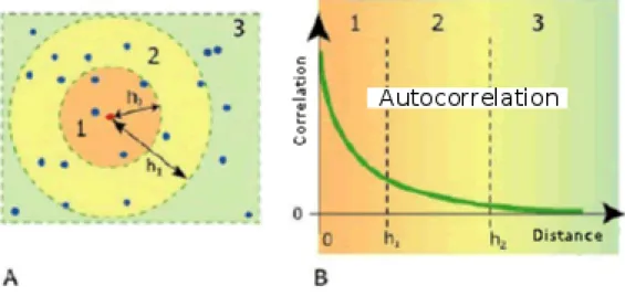
The autocorrelation defines the degree of spatial dependence between the values of a sampled variable. An intuitive feature of the environment is that its properties are related to each other in a any scale, large or small, fig. 2.1. It means that sampled values in locations close to each other, tend to have similar behavior, while values of the same variable measured in samples collected in areas remote one from the other have different behaviors, or at least tend to differ from the average values found in two places. In this sense, the correlation between the values of the variable tends to decrease with increasing distance. Adopting the stochastic point of view, each point in space has not only one value for a property, but a whole set of values. Thus the observed value becomes a value taken at random from an infinite number of possible values, taken from some probability distribution for the same the law. This means that at any point in space there is a change. Thus for each point X0 and a property

Z(X0) is treated as a random variable, generally continuous and not discrete, with its

own mean (µ), a variance (σ2) , moments of higher order and a cumulative probability function of density. This variable therefore has a probability distribution from which the real value is extracted. the set of real Z values (measured) can be considered as a

(28)

2.2 Geostatistic

Figure 2.1: Relationship between very close samples correlated, 1, distant low correlation, 2, distant and not correlated, 3, with the point considered (A) and relationship between distance and correlation, or autocorrelation (B), from (164)

regionalized variable as it is a variable whose value is strongly influenced by the spatial position. Considering Z(x) the regionalized variable in x position, is possible to write:

Z(x) = a + R(x)

where a is the random component and R(x) the regionalized component. When a is dominant against R(x) the variable is studied with the classical statistical methods. Otherwise it falls within the geostatistics field. A stationary process is a stochastic process where the probability density function of one random variable Z it doesen’t change neither in time nor in space, thus parameters mean and variance do not change over time and space, consequently the distribution of the random process maintains the same attributes everywhere. Supposing we measure a regionalized variable Z in a particular direction in space obtaining certain values for each point in this direction it is possible to get a pattern of values similar to that shown in fig. 2.2 (A). As it can be seen in fig. 2.2 (B), there is a systematic change of the average value of the variable, relevant to the scale of observation, and then we can no longer assume a stationary

(29)

2.2 Geostatistic

Figure 2.2: Z(x) values along a particular direction of space (A) and subdivision of the total variability into two components (B), from (164)

average or stationary model. This condition of non-stationarity of the variable values is the sum of two components:

• drift (systematic increase of the mean value)

• residual (variability around the systematic component)

The drift is essentially the average value of the variable as a function of location in which the variable was measured and can be written as m(x). The value of the variable Z for each point x can then be expressed as the sum of the average point x and the deviation from the mean value measured, Y (x):

Z(x) = Y (x) + m(x)

The assumptions made are as follows:

• Y (x) residual is a random stationary variable, where the mean value is constant • the drift is a deterministic function of the localization

• the drift and residual are not correlated

The semivariogram is a geostatistical algorithm which is used to evaluate the spa-tial autocorrelation of gereferenced data points observed. The semivariogram function

(30)

2.2 Geostatistic

interpolates the semi-variable of observed values in groups of pairs of points at certain distances (lag) according to a certain direction.

The semi-variable is:

γ(h) = 1 (2m(h)) m(h) X i=1 (Z(xi+ h) − Z(xi))2

where Z is the value of a measurement at a particular point, h is an interval of distance between points measurement (lag) and m(h) represents the number of pairs of observations at a distance h. The axes of the experimental semivariogram are distances between pairs of data (x axes) and semi-variance (y axes), fig. 2.3. The graph obtained

Figure 2.3: Semivariogram function example, from (164)

from the semi-variable equation consists of a series of distinct points, distant from each other a certain lag defined. The experimental semivariogram must be interpolated with different mathematical functions, to determine the type of spatial autocorrelation of the measured variable, which will subsequently be used interpolation with kriging. In the process of kriging in fact a continuous function is required for the assignment of weights at all points, and is linked to the value of the semi-variable. The semivariogram model is inferred from observation of the experimental semivariogram.

(31)

2.2 Geostatistic

It is possible to imagine a function that best approximates the experimental points of the variogram; the problem is to understand how this curve will follow the experimental data. To model and have a good result on the variogram it is important to pay attention on the general trend points and not on the individual fluctuations. Then the type of function to be chosen has to be as simple as possible, and always in relation to the complexity of the variogram. The extimated parameters are:

• nugget: describe the level of random variability

• sill: the maximum semivariance value when we have the stationary condition (it approximates to the excess sample variance)

• range: the maximum distance within which correlation of semi-variable and lag are manifested

The semivariogram function is a spatial correlation function, with certain graphic and quantitative characteristics, called structural properties, as:

• symmetry • continuity

• range of influence • behavior near the origin • anisotropy

• drift

The modeling of the variogram is a very delicate step as it is necessary to choose the curve that better approximates the discrete number of points obtained from the experimental variogram. The process of model fitting to the variogram is difficult for various reasons:

1. the accuracy of the observed semi-variable is not constantly 2. The variogram can contain many point to point fluctuations

For these reasons a fitting model procedure is recommended it includes both the visual appearance in the trend function and the statistical aspect, as follow:

(32)

2.2 Geostatistic

1. create the experimental variogram

2. chose one or more of the available models in order to meet the main trends of the experimental values

3. adapt the model with statistical procedures to minimize errors

4. check the graph result in order to assess qualitatively the goodness of the result There are many kinds of model to approximate the experimental variogram 2.4, the most widely used are:

• exponential model • spheric model • gaussian model • linear

(33)

2.2 Geostatistic

The estimation of the variogram function is performed on the basis of data from sampling the phenomenon under study. If you sampled data according to a regular grid, computing is very simple owing to the stationarity of the increase Z(x + h) − Z(x), calculation is immediately the variogram function for a certain direction and for a particular lag h. The variogram calculation is based on the differences in the values of the variable regionalized in two different locations, separated by a distance h. The procedure is:

1. start calculating the difference between the values z(x1) and z(x2), then between z(x2) and z(x3), for the couple z(xi− 1) and z(xi). The different will be equal

to m(x), ie the number of pairs of samples for this lag 2. the result of any differences rises to the square

3. add up all the squares

4. divide this sum by 2m(h), as into the semivariogram formula 5. repeat the same steps from 1 to 4 second lag (double the first) 6. repeat the same steps from 1 to 4 third lag (three times the first) 7. repeats the procedure until the last lag distance you want

Usually you choose a number of lag ranging from 10 to 20. In fact, a low number of lag (less of 10) might result in loss of meaning to the variogram, lowering the resolving power of the variogram. A high number of lag would lag too much to be considered beyond the maximum range of spatial correlation among the data. Unfortunately there is not always a regular grid, of samples do the technical for the calculation of the variogram has to be adjusted. In this case it may happen that in a certain direction r no point fall sampled, because it is arranged in an irregular manner. To avoid this, we consider one direction r, detected using an angle from a reference direction, with an angular tolerance ∆Φ, fig. 2.5. ∆h tolerance must also be given on the distance. So by all pairs with distance between h − ∆h and h + ∆h and aligned in the direction between Φ − ∆Φ and Φ + ∆Φ contribute to the calculation of the variogram. The values of the tolerances to be taken of course depend on the amount of samples you have: more such

(34)

2.2 Geostatistic

Figure 2.5: Irregular sampling, from (164)

samples may be smaller and tolerances, allowing a greater precision in the calculation of the variogram.

The map of the variogram is a plot representing the progress of the variance in space it. Is constructed, using a grid of square cells (or circular sectors), based on the values the y axis of the experimental variogram. The width of the cells is determined by the extent of the lag, the higher the number the smaller cells lag. The map of the variogram makes it understandable quickly how the anisotropy vary in the space to decide on which direction the main focus with the variogram. Each map cell is represented, in fact, with a variable color symbolism depending on the value of the variogram according to its chromatic scale, fig. 2.6.

This plot, as mentioned before, allows to define the most continuity data direc-tion, simply watching from the center and identifying the direction from which they have lower values of variance. This different pattern of spatial variability is known as anisotropy.

The cross-validation is an iterative procedure: each sample is excluded from the dataset and interpolated through the value of others, using the variogram model you want to test. The comparison between the estimated value and the actual value is called the residue of the cross-validation. The study of residues in the dataset shows us the model behavior. The main parameters study are:

1. the mean residuals, indicating the accuracy of the estimate, which must be close to zero

(35)

2.2 Geostatistic

Figure 2.6: Example of a map of the variogram, from (164)

2. the least squares error (RMSE), indicating the precision q

1 n

Pn

i=1(Zi− Z0)2, that

must be the smallest possible

3. the standard deviation of the kriging (MSDR) _n1Pn i=1

(Zi−Z0)2

σ2 , which allows to compare the magnitude of errors predicted with errors actually committed, com-paring the variance that is true and calculated in the cross-validation.

where Zi is the estimated i-th value, Z0 is the real values, σ2 the error variance and n

the samples number.

In order to reconstruct the sought surface it is necessary to interpolate the available data to estimate the values whose you do not have samples. In this sense, the kriging comes to us as it gives a solution to the problem of estimating based on a stochastic continuum model of spatial variation. It makes the best use of knowledge of the variable, taking into account the way how a property varies in space through the variogram model that was chosen and validated. There are different types of kriging, including ordinary kriging (OK) and universal kriging (UK), for different types of variables. What differentiates them is the type of variable used: Ordinary kriging can only work with stationary variables of the second order (present constant mean and variance depending only on the lag moving from point to point), universal kriging can also work with non-stationary variables (which have a drift). As mentioned before one of the assumptions

(36)

2.2 Geostatistic

made in the ordinary kriging is the stationarity of the data to estimate, this means that moving from one area to another the average of the values is almost constant. When there is a significant trend of the data space (intrinsic feature of the data itself that causes the average of the values is not constant but varies from point to point) this assumption is not valid. The stationarity condition of the data can still be restored through the introduction of a deterministic function describing the drift, that is the trend of the average, in order to isolate the residual, that is the part of the aleatory data. The universal kriging model subtracts the drift from the data, by a deterministic function, and analyzes the only residual component. As the drift and the residue are not correlated the drift can be modeled by a deterministic function of the localization, therefore the value of the variable Z(x) is:

Z(x) = K X k=0 akfk(x) + m(x) where K X k=0 akfk(x)

is the sum of a polynomials functions set fk(x) of order 1 or 2 and f0(x) = 1 and the

m(x) term is the stocastic component (variogram).

The universal kriging, used in the non-stationarity, provides the point estimated (the point x0) by the formula:

z ∗U K(x0) = K X k=0 n X i=1 akλifk(xi)

that will provide a correct estimate only if it meets the condition:

n

X

i=1

(37)

2.2 Geostatistic

The solution of the system below allows to quantify the weights λj to estimate the

generic point: n X i=1 λiγ(xi, xj) + ψ0+ K X k=0 ψkfk(xi) = γ(xi, x0) ∀i = 1, .., N n X i=1 λi = 1 n X i=1 λifk(xi) = fk(x0) ∀k = 1, .., K

where γ(xi, xj) is the semi-variable residues between points xi and xj and γ(xi, x0)

is the semi-variable between the i-th sampled point and the target point of the estimate x0. In kriging, ordinary and universal, through a system of linear equations, assigning

weights to the analyzed samples surrounding the point that minimizes the total variance of errors. Usually four or five closest samples contribute 80 % of the total weight, the remaining 20 % is awarded to approximately ten other nearby points. The main factors that influence weights are:

1. closer samples carry more weight than the far ones and the amount of weight depends on their position and on the variogram;

2. samples grouped around a certain point carry less weight than isolated.

Just to remember, in the multivariate statistical analysis, the method is known as cokriging interpolation. This method is very similar to ordinary kriging, the only difference is that in estimating the main variable (target) is not only based on the values of the variable examined but it also considers other auxiliary variables. Considering the case where you have two spatially correlated variables Z1(x) and Z2(x), sampled

respectively in a set of n1 and n2 locations, wishing to estimate the value of the variable

Z1(x0) through the values of surrounding Z1(x) and Z2(x) use:

z ∗ (x0) = n1 X i=1 λiz1(xi) + n2 X i=1 ωiz2(xi)

(38)

2.3 Used data

where λi and ωi represent the weights of the two variables considered. The value of

the weights to be assigned is found by solving the system below:

n1 X j=1 λjγ1(xi, xj) + n2 X j=1 ωjγ12(xi, xj) + µ1 = γ1(xi, x0) n1 X j=1 λjγ12(xi, xj) + n2 X j=1 ωjγ2(xi, xj) + µ2 = γ2(xi, x0) n1 X j=1 λj = 1 n2 X j=1 ωj = 0

The cokriging is therefore useful when the main variable is under-sampled compared to the other.

2.3 Used data

The data choice is obviously the first important aspect to be evaluated in order to de-velop the proposed target, the need to find the useful data to build 3D geologic model is an hard work, that is for the sensibility of the data required. The building of 3D geologic model starts, for sure, from a geologic surface map in a certain scale (estimated valid for a precise scale of work), then it would be important to have surveys that reach depths considered of interest for you to reconstruct 3D surface (direct data). Always it is not easy to find out the data well log need, those are clearly industrial sensible data, in this case, and when we are lucky, is possible relay on indirect investigations coming from geophysics methods, that means seismic data, gravimetric data or magnetic data. It is evident, we are against a various dataset, one of the project target is to organize this data collection in order to make this heterogeneous information easily available. In particular there were collected data about geological surface map with the most

(39)

2.3 Used data

important geological domains and structural features, some geothermal and hydrocar-bons well logs (onshore and offshore) and finally also a geophysical data on seismic and gravimetric sources. This organized dataset allows to develop the geologic models to improve the knowledge on crystalline basement, their sedimentary meso-cenozoic covers in the study area, and helps to identify, define and evaluate any potential reservoirs of geo-resources. Below the data collected and how they were organized are described.

2.3.1 CROP data

In order to build the model of the Variscan basement surface seismic data were sought, they covered the Italian peninsula area and ensured a depth of investigation and a uniform consistency of the information on a small scale, a large amount of data has been extracted from the (87) and the attached tables. Unlike the volume (183), where the seismic cross-section are not interpreted, in the volume (87) is possible to find the cross seismic section with the authors interpretation. The reinterpretation of the seismic data, despite having scientific interest, was not included among the aims of the project, both because of the difficulties related to the reprocessing of seismic data and its geological interpretation effects, and for the short notice of this project. The (87) contains, as well as a book with scientific papers relating to the work of seismic interpretation and geodynamics,the base map with the tracks of the seismic profile distributed in the Italian peninsula and surrounding seas, a set of seismic interpreted profile and a map of the Moho obtained from interpretation of the same profiles of the Italian area.

The first step in the acquiring CROP data process includes the scanning operations of the base map and the subsequent georeferencing operation. Then, with QGIS soft-ware 2.1.3, the profiles were drawn and saved in a shape file. The Moho map, after the scanning and georeferncing operations, has always been digitized in shape format. The digitizing process, topologically realized, produced a line layer representing the Moho’s isobaths, the attribute related table is compiled with the values of each line. Was also produced another vector layer which reproduces the most important tectonic lineaments that involve the moho discontinuity. The CNR Institute of Marine Sciences (ISMAR), is the institution responsible for maintenance and data management CROP, so ask them the ascii dataset of some seismic profiles of interest. For our purpose it was important to have the exact location of each shot point (SP) belonging to each

(40)

2.3 Used data

profile of interest. The received data contains the latitude and longitude of each SP, so with the QGIS software it was possible to plot each SP in each own profile in order to obtain the data map, starting point of all the further elaborations. This kind of data was used mainly to build the model explained in chapter 4.

2.3.2 BDNG data

The underground data were acquired from a part of the Italian National Geothermal Database (BDNG), in particular these data are represented by the stratigraphic well data contained therein, where surveys related to levels reached lithologies belonging to the crystalline basement and its related. The Italian National Geothermal Database was built in 1993 by the International Institute for Geothermal Research in Pisa (cur-rently IGG, Institute of Geosciences and Earth Resources) of the National Research Council (C.N.R.) as completion of the Inventory of geothermal resources by CNR, ENEA, ENEL and ENI, under Law No 896 of 1986. Data have been continuosly up-dated until 2001. During 2008, a software and data update have been scheduled and implemented with the help and technical support of ENI Refining & Marketing, R & S managment. The BDNG is a part of a wide project, called Geothopica, where the database is the indispensable core. The commitment of the Institute of Geosciences and Earth Resources, with the support of ENI Refining & Marketing, R & S managment, and with collaboration of UNMIG (Ufficio Nazionale Minerario per gli Idrocarburi e le Georisorse National Office for Mining Hydrocarbons and Earth Resources) department of the National Economic Development Ministry, that guaranteed the access to a new dataset, has produced an upgrade that yields one of the most complete underground data repository at the national level. The database contains geothermal data for the whole Italian territory, such as geothermal wells, geothermal springs or manifestation (with temperature > 30◦C), geothermal exploration wells, hydrocarbons wells and also shallow and unproductive exploration wells. After the last update (winter 2010), 3183 wells and 586 thermal springs are stored in the database. At present the BDNG is hosted in a computer server where each client, who has a right authorization, is able to access the dataset. That’s a tipycal client-server architectures, characterized by high storage capacity, data processing and data sharing between a wide spread users typol-ogy. The server side contains the database server software and the data stored providing

(41)

2.3 Used data

enterprise features such as referential integrity constrain, query and search highly per-forming algoritms, data managment, multi user connection without inteferences, user access policy, data recovery.

2.3.3 Geological map

Particular attention was dedicated to the geological map to take into account, the choice of the geological map is a crucial step in order to define what are the litho-stratigraphic units to correlate to the wells selected litho-stratigraphy. The first geological map col-lected and studied was the Geological Tuscan Region map in 1:250.000 scale, published in 2004 (32), but this map was not sufficient for the whole national territory, because it has a too large scale for the national representation and it faults of course for the missing coverage outside the Tuscan region. At first, the Geologic Structural Model of Italy at 1:500.000 scale (2), seemed to satisfy the specific requirements, but at a more detailed analysis of results as well as always be too detailed for the realization of the model of the surface of the Variscan basement. The ISPRA (Superior Institute for the Protection and Environmental Research) 1:1.000.000 scale geological map (111) seems to satisfy the requirements such as a good scale of the representation for the study area, a good litho-stratigraphical division correlates with the lithostratigraphic wells acquired easily.

2.3.4 Geophysical data

Now geophysical dataset includes only gravimetric data, the magnetic data are not available because belonging to ENI, also after a formal request made for scientific use, the ENI headquarter has not released any kind of magnetic data.

Otherside, on the ISPRA website is possible to find out some gravimetric data output, this dataset is available free of charge for downloading. The gravimetric data includes Bouguer Anomalies vector isoline, raster grid and georeferenced images, but only the station position are present, the measured data in each station is missing. The Italian territory is cover by 39 map sheets at 1:250.000 scale (112), in particular the observed data stored in the postgresql database, with spatial postgis extention, was referred to IGSN71 (International Gravity Standardization Net 1971)and the Bouguer Anomalies were computed with a correction density of 2,63 g/cm3 The gravimetric map

(42)

2.3 Used data

is the result of a project that involves ISPRA, National Institute of Oceanogrphy and Sperimental Geophysic (OGS) and Exploration and Production division of ENI.

(43)

3

The geology of the Italian area

3.1 The evolution of appennine’s tectonic

The geology of Italy is the result of a really complex geological history that can be traced from the late Paleozoic Variscan orogen, throughout the Mesozoic opening of the Paleo-Tethys with progressive crustal thinning and development of a series of platforms and basins sometimes evolved into the oceanic stage e.g. (22, 189) with the sedimentation of widespread and thick Mesozoic carbonate platforms grown on continental margins e.g. (145, 189) and the closure of continental and oceanic basins developed within the frame of convergence between Africa and Eurasia during the Tertiary (22, 125, 172). The present day tectonics of Italy is still controlled by the relative motions between Africa and Eurasia plates Fig. 3.1, accommodated by the displacement of a number of tectonic units that developed during the collision of the Alpine and Apennine belts (21, 72, 76, 125, 160).

The Apennines, constitute the backbone of peninsular Italy, form a NW-trending, ENE-vergent, foldthrust belt, Fig. 3.2.

In their frontal part, the Apennines belt is limited by the foredeeps that developed to the east from Southern Apennines to the Po Plain. Following the Oligocene-Miocene continental collision, clastic wedges accumulated in these elongated foreland basins in front of the deforming belt. During Neogene, contractional deformations migrated east-ward, mostly in a piggyback sequence of thrusting towards the foreland (62) favoured by the parallel retreat and the sinking of the lithosphere toward the Adriatic foreland (125).

(44)

3.1 The evolution of appennine’s tectonic

Figure 3.1: Western Mediterranean paleotectonic maps, from (145). Brown area: conti-nental crust. Green area: oceanic crust. The red arrows are the regional trascurrent faults (in A and B), the red line with red triangles indicates subduction lineaments. The double red arrows indicate the opening of the provential-ligurian basin (C) and the Tyrrhenian basin (D)