On the problem of checking chase termination

(1)

(2)

UNIVERSIT `

A DELLA CALABRIA

Facolt`

a di Ingegneria

Dipartimento di Elettronica, Informatica e Sistemistica

Dottorato di Ricerca in Ingegneria dei Sistemi ed Informatica

XXIV ciclo

Settore Scientifico Disciplinare ING/INF-05

Tesi di Dottorato

ON THE PROBLEM OF CHECKING

CHASE TERMINATION

Coordinatore

Prof. Luigi Palopoli

Supervisore

Prof. Sergio Greco

Francesca Spezzano

(3)

(4)

Preface

Several database areas such as data exchange and data integration share the problem of fixing database instance violations with respect to a set of in-tegrity constraints. The chase algorithm solves such violations by inserting tuples and setting the value of nulls. Unfortunately, the chase algorithm may not terminate and the problem of deciding whether the chase process termi-nates is undecidable. In recent years, the problem know as chase termination has been investigated. It consists in the detection of sufficient conditions, derived from the structural analysis of dependencies, guaranteeing that the chase fixpoint terminates independently from the database instance. Several criteria introducing sufficient conditions for chase termination have been re-cently proposed (weak acyclicity, stratification, super-weak acyclicity, induc-tive restriction, etc.). Most of these criteria concentrate on tuple generating dependencies (TGDs).

The aim of this thesis is to present more general criteria and techniques for chase termination.

We first present extensions of the well-known stratification criterion and in-troduce a new criterion, called local stratification (LS), which generalizes both super-weak acyclicity and stratification-based criteria (including the class of constraints which are inductively restricted).

Next the thesis presents a rewriting algorithm transforming the original set of constraints Σ into an ‘equivalent’ set Σα _{and verifying the structural}

properties for chase termination on Σα_{. The rewriting of constraints allows}

to recognize larger classes of constraints for which chase termination is guar-anteed. In particular, we show that if Σ satisﬁes chase termination condition

C, then the rewritten set Σα_{satisﬁes C as well, but the vice versa is not true,}

that is there are signiﬁcant classes of constraints for which Σαsatisﬁes C and

Σ does not.

A more general rewriting algorithm producing as output an equivalent set of dependencies and a boolean value stating whether a sort of cyclicity has been detected is also proposed. The new rewriting technique and the checking of acyclicity allow us to introduce the class of acyclic constraints (AC), which

(5)

VI Preface

generalizes LS and guarantees that all chase sequences are ﬁnite with a length polynomial in the size of the input database.

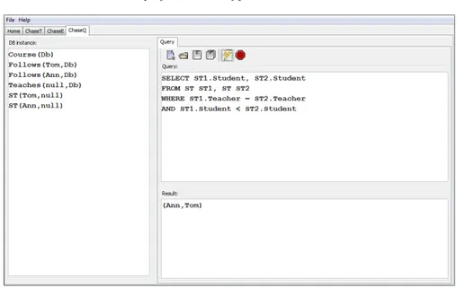
Finally, a system prototype that allows users to design data dependencies and apply diﬀerent criteria and algorithms for checking chase termination is presented. The tool is also able to execute the chase procedure in order to repair the possible incomplete database provided by the user, and to execute (restricted) SQL queries over the repaired database.

Acknowledgments

My full gratitude goes to my supervisor Prof. Sergio Greco for his excellent and always present guidance during my doctoral course and all opportunities oﬀered to me.

A special thank to my colleague and friend Irina Trubitsyna for her help and good suggestions.

I am also grateful to Prof. Phokion Kolaitis for giving me the opportunity to spend a year abroad at UCSC, and have interesting research meetings with him.

Last but not the least, I would like to thank for their support my Mum and Dad, my sister Annachiara and my love Edoardo.

Rende,

(6)

1 Introduction

The Chase is a fixpoint algorithm enforcing satisfaction of data depen-dencies in databases. It has been proposed more than thirty years ago [ABU79, MMS79] and has received an increasing attention in recent years in both database theory and practical applications. Indeed, the availability of data coming from different sources easily results in inconsistent or incomplete data (i.e. data not satisfying data dependencies) and, therefore, techniques for fixing inconsistencies are crucial [Ber06, Cho07]. The chase algorithm is used, directly or indirectly, on an everyday basis by people who design databases, and it is used in commercial systems to reason about the consistency and correctness of a data design. New applications of the chase in meta-data man-agement, ontological reasoning, data exchange and data cleaning have been proposed as well [BKL11, CGP10, DLLR07].

The execution of the chase algorithm involves the insertion of tuples with possible null values and the changing of nulls which can be made equal to constants or other null values. However, the insertion of tuples with new (null) values could result in a non-terminating execution. The following example shows a case where a given database does not satisfy a set of data dependencies (also called constraints) and the application of the chase algorithm produces a new consistent database by adding tuples with nulls.

Example 1.1. Consider the set of constraints Σ1.1: ∀x N(x) → ∃ y E(x, y) ∀x∀y S(y) ∧ E(x, y) → N(y)

where the relations N and S store normal nodes and special nodes, respec-tively, whereas E stores edges. The second constraint states that if there exists an edge from x to y and y is a special node, then y must also be a (normal) node. The ﬁrst constraint states that every normal node must have an outgo-ing edge.

Assume that the database contains the tuples S(a), E(b, a). Since the se-cond constraint is not satisﬁed, the tuple N (a) is inserted. This update

(9)

ope-2 1 Introduction

ration ﬁres the ﬁrst constraint to insert the tuple E(a, n1), where n1 is a

new labeled null. At this point the chase terminates since the database is consistent, i.e. the second constraint cannot be ﬁred because n1 is not in

the relation S. The output database is consistent as both dependencies are

satisﬁed. 2

However, it is important to observe that if we delete the atom S(y) from the second constraint, the chase will never terminate as an inﬁnite number of tuples will be added to the database.

The problem recently investigated, known as chase termination, consists in the identification of sufficient conditions, based on structural properties of the input set of constraints, guaranteeing that the chase fixpoint terminates independently from the database instance.

Several criteria guaranteeing chase termination for all chase sequences and for all database instances have been recently deﬁned.

Fagin et al. [FKMP05] introduced the class of weakly acyclic sets of con-straints (W A). Informally, weak acyclicity checks that the set of concon-straints does not present cyclic conditions for which a new null value forces (directly or indirectly) the introduction of another null in the same position. In the previ-ous example we have that the presence of a value in N1, i.e. in the ﬁrst position

of the predicate N , forces the introduction of a new null value in position E2,

i.e. in the second position of the predicate E, and it is denoted as N1→∗ E2;

this value is then introduced in position N1(denoted as E2→ N1) and next a

new null value is introduced in E2. The cycle going through the special edge N1→∗ E2means that an inﬁnite number of nulls could be introduced.

The class of weakly acyclic sets of constraints has been generalized in several works [DNR08, Mar09, MSL09a].

Deutsch et al. proposed an extension of weak acyclicity called stratification (Str) [DNR08]. The idea behind stratification is to decompose, by construct-ing a chase graph, the set of constraints into independent subsets, where each subset consists of constraints that may fire each other, and to check each com-ponent separately for weak acyclicity. However, in [MSL09b] it has been shown that stratification is not able to check termination of all chase sequences , but it is sufficient to state that if a set of constraints is stratified, then there is at least one terminating chase sequence which can be determined from the chase graph. Thus, a variant of stratification, called c-stratification (CStr) [MSL09b], has been proposed to guarantee the termination of all chase se-quences.

Meier et al. proposed a different extension of weak acyclicity called safety (SC) [MSL09a]. The improvement is based on the fact that only the effective propagation of null values should be considered in the graph. Thus, a variable can propagate nulls only if all its occurrences appear in ‘affected’ positions, i.e. positions which may actually contain null values [CGK08]. The Example 1.1 presents a set of constraints which is both safe and stratified, but not weakly acyclic. In fact, according to the safety condition, we have that E2 does not

(10)

1 Introduction 3 propagate null values to N1 as the variable y also appears in the relation S

which does not contain null values. So, position N1 cannot contain nulls, i.e.

it is not affected. From the motivation that S cannot contain null values, we have that firing r1cannot cause r2 to fire, and then Σ1.1 is also stratified.

Stratiﬁcation and safety are not comparable (i.e. there are sets of con-straints which only satisfy one of the two criteria), but are both generalized by the inductive restriction (IR) criterium [MSL09a, MSL09b].

A diﬀerent extension of weak acyclicity, not comparable with inductive restriction, has been introduced in [Mar09] under the name of super-weak

acyclicity (SwA). Basically, SwA takes into account the fact that variables

may appear more than once in body atoms of constraints and, therefore, when diﬀerent nulls are inserted in positions associated with the same variable, constraints are not ﬁred.

The idea underlying stratification, also used in its variation and exten-sions (CStr and IR) and in the super-weak acyclicity, is to consider, in the propagation of nulls, how constraints may fire each other. However, there are simple cases where current criteria are not able to understand that all chase sequences are finite.

Example 1.2. Consider the following set of constraints Σ1.2 consisting of the

TGD

∀x∀y E(x, y) ∧ E(y, x) → ∃z E(y, z) ∧ E(z, x)

We can distinguish two cases. If we suppose to have a database instance

D1 = {E(a, b), E(b, a)} we have that the TGD is not satisﬁed, but the

constraint will be applied only once by the chase as the resulting database

D′₁={E(a, b), E(b, a), E(b, η1), E(η1, a)} is consistent. Otherwise, if we

sup-pose to have a database instance D2={E(a, a)}, it is already consistent, and

no chase step will be applied. It is easy to see that the chase is always termi-nating for all database instances, but none of the existing criteria guaranteeing the termination of all chase sequences is able to recognize it as terminating.2 In order to cope with this problem, we propose extensions of the well-known stratiﬁcation criterion and then introduce a new criterion, called

local stratiﬁcation (LS), which generalizes both super-weak acyclicity and

stratiﬁcation-based criteria (including the class of constraints which are in-ductively restricted) and guarantees the termination of all chase sequences, for all database instances, in polynomial time.

Nevertheless, despite the previously mentioned results, there are still im-portant classes of terminating data dependencies which are not identiﬁed by none of the previous mentioned criteria.

Example 1.3. Consider the set of constraints Σ1.3: ∀x N(x) → ∃y E(x, y) ∀x∀y S(x) ∧ E(x, y) → N(y)

(11)

4 1 Introduction

that is a variant of Example 1.1 where the second constraint states that if there exists an edge from x to y and x is a special node, then y must be a (normal) node. Assume that the database contains the tuples S(a), N (a). The ﬁrst step of the chase algorithm will add the tuple E(a, n1), where n1is a new

labeled null, to the database. At this point, since the second constraints is no more satisﬁed, the second constraint ﬁres to insert the tuple N (n1) which

in turn ﬁres the ﬁrst constraint so that the tuple E(n1, n2) is added to the

database. At this point the chase terminates (since the the tuple S(n1) is not

in the database), and both dependencies are satisﬁed. 2 Thus, we present an orthogonal technique which enlarges the classes of dependencies recognized by the above criteria. This technique rewrites the input set of constraints Σ into an equivalent, but more informative, set Σα

and checks classical criteria satisfaction on Σα_{. The rewriting of constraints}

allows to recognize larger classes of constraints for which chase termination is guaranteed. In particular, we show that if Σ satisfies chase termination conditions C, then the rewritten set Σαsatisfies C as well, but the vice versa is not true, that is there are significant classes of constraints for which Σα satisfies C and Σ does not.

In the presence of constraints that are TGDs and EGDs, the previous described criteria and technique are quite weak, as it may happen that a solution can be found even if the set of TGDs are non-terminating.

Example 1.4. Consider the set of constraints Σ1.4, stating that each node has

an outgoing edge (r1), each edge ends in a node (r2) and the resulting graph

must contain at most one node (EGD r3).

r1: ∀x N(x) → ∃y E(x, y) r2: ∀x ∀y E(x, y) → N(y) r3: ∀x ∀y N(x) ∧ N(y) → x = y

The alternating application of constraints r1 and r2 (r1, r2, r1, r2, . . .) could

be not terminating, whereas the alternating application of constraints r1, r2

and r3(r1, r2, r3,· · · ) always terminates. Indeed, assuming that the database D contains only the tuple N (a), a solution for D and Σ is obtained by

intro-ducing the tuple E(a, a). This solution is obtained as follows: by applying the ﬁrst constraint which is not satisﬁed, the tuple E(a, η1) is introduced. Then,

from the second constraint, the tuple N (η1) must also be inserted. At this

point the application of the third constraint updates the null value η1 to a.2

Thus, the right selection of dependencies to be applied could inhibit the ﬁring of constraints which may cause the cyclic introduction of null values, guaranteeing the presence of at least one terminating chase sequence.

Contributions

(12)

1 Introduction 5

• We ﬁrst analyze the relationship among current criteria and show that

super-weak acyclicity is not comparable with (c-)stratiﬁcation, but it ex-tends safety.

• We analyze the stratiﬁcation conditions and propose a new stratiﬁcation

criterion, called WA-stratiﬁcation, which builds a diﬀerent chase graph

Γ (Σ), called ﬁring graph, and overcomes some limitations of both

stratifi-cation and c-stratifistratifi-cation; since WA-stratifistratifi-cation checks weak acyclicity over strong components of Γ (Σ), two further, more powerful, conditions checking safety and super-weak acyclicity over Γ (Σ) are defined. These criteria are called SC-stratification and SwA-stratification.

• SwA-stratiﬁcation, the most general of the above new criteria, is not

comparable with inductive restriction. Thus, we propose a further cri-terion, called Local stratification (LS) which uses more refined conditions of SwA during the construction of the firing graph. LS generalizes SwA-stratification and is more powerful than IR.

• As a minor result, since our criteria are based on the construction of a

fir-ing graph, an algorithm solvfir-ing the firfir-ing problem (i.e. checkfir-ing whether a constraint r1 could fire a constraint r2) is presented. It is shown that,

although its complexity is exponential in the number of atoms in the body of r2, because it depends on the number of atoms in the head of r1

uni-fying with each single atom in the body of r2, for some standard classes

of constraints (e.g. multivalued dependencies, inclusion dependencies) it performs very well (recall that the ﬁring problem for the (c-)stratiﬁcation criterion is inN P [DNR08, MSL09a]).

• Next, we present a technique for rewriting a set of constraints into an

‘equivalent’ set by adorning predicate symbols and show that the checking of termination criteria over the target set allows to detect larger classes of source constraints for which all chase sequences terminate;

• We extend the rewriting technique to capture even larger classes of

con-straints for which the chase terminates by analyzing affected positions (positions which may hold nulls); this is carried out by adorning predi-cates and using different adorning symbols in cases where we can statically establish that two affected positions cannot contain the same null value;

• The rewriting technique permits us to introduce a new class of terminating

constraints consisting of a set of dependencies which are detected as acyclic by our rewriting algorithm. This class, called Acyclic (AC) generalizes LS and, considering static criteria for checking chase termination, is the most general criterion so far proposed1_.

• Checking termination criteria and rewriting techniques have been

imple-mented into a system prototype downloadable from the web. This system also allows to execute the chase ﬁxpoint to repair and querying a given database on the base of the input dependencies.

1

In this thesis we will use calligraphic style C in order to denote the terminating class of constraints recognized by criterion C.

(13)

6 1 Introduction

Organization

This thesis is organized as follows.

Chapter 2 introduces the basic notions that we shall use throughout the thesis.

Chapter 3 presents the chase algorithm and its variants and gives a survey on the well-known chase termination criteria proposed in the literature. In particular, weak acyclicity, safety, (c-)stratiﬁcation, super-weak acyclicity, safe restriction and inductive restriction are explained.

Chapter 4 discusses several problems and applications using the chase al-gorithm, namely implication of data dependencies, database design, query optimization, query answering and containment under constraints, data inte-gration and data exchange.

Chapter 5 presents some improvements for termination conditions dis-cussed in Chapter 3 and then describes the class of locally stratiﬁed depen-dencies, that generalizes previously known classes, for which termination of the chase algorithm is guaranteed.

Chapter 6 presents a technique for checking chase termination based on rewriting the original set of TGDs into an ‘equivalent’ set Σα_{, whose}

struc-tural properties allow to detect larger classes of source constraints for which all chase sequences terminate. Section 6.2 extends the rewriting technique by analyzing aﬀected positions (positions which may hold nulls) and by intro-ducing cyclicity detection in the rewriting process. This approach allows us to further enlarge the class of terminating dependencies and obtain the most general criterion so far proposed.

Chapter 7 brieﬂy presents ChaseTEQ, a system prototype available on the web which implements some of the criteria and techniques for checking chase termination presented in this thesis, and allow the user to repair and querying the possible incomplete database.

Finally, in Chapter 8 conclusions are drawn.

Summary of Publications

Some of the results presented in this thesis appeared in the conference papers [GS10], presented at the 36th International Conference on Very Large Data

Bases (VLDB 2010) and [GST11] presented at the 37th International Confer-ence on Very Large Data Bases (VLDB 2011). The system prototype has been

presented in [DST11] at the 19th Italian Symposium on Advanced Database

Systems (SEBD 2011) and in [DGST11] at the 5th International Conference on Scalable Uncertainty Management (SUM 2011).

(14)

2 Theoretical Background

In this chapter we deﬁne the basic notions that we shall use throughout the thesis.

2.1 Relational Model

We introduce the following disjunct sets of symbols: (i) an infinite set Consts of constants, (ii) an infinite set N ulls of labeled nulls and (iii) an infinite set

V ars of variables.

A relational schemaR is a pair ⟨R, Σ⟩ where:

• R is a set of relational predicates R, each with its associated arity ar(R)

that indicates the number of its attributes X, and

• Σ is a set of (integrity) constraints expressed on the relations in R, i.e.

assertion on the relations in R that are intended to be satisﬁed by database instances.

When no integrity constraints are deﬁned in R, we simply denote the relational schema with R.

An instance of a relational predicate R of arity n is a set of ground atoms in the form R(c1, . . . , cn), where ci ∈ Consts ∪ Nulls. Such (ground) atoms

are also called tuples or facts. A database instance, or simply an instance or a database, for a relational schema R = ⟨R, Σ⟩ is a set of instances for the relations in R. A database instance for a schema R is said to be

con-sistent with R if it satisﬁes all constraints expressed on R. We denote by D a database instance constructed on Consts and by J, K the database

in-stances constructed on Consts∪Nulls. Given an instance K, Nulls(K) (resp.

Consts(K)) denotes the set of labeled nulls (resp. constants) occurring in K.

An atomic formula (or atom) is of the form R(t1, . . . , tn) where R is a

rela-tional predicate, t1, . . . , tn are terms belonging to the domain Consts∪ V ars

(15)

8 2 Theoretical Background

Let K be a database over a relational schema R and S ⊆ R, then

K[S] denotes the subset of K consisting of instances whose predicates are

in S (clearly K = K[R]). Analogously, if we have a collection of databases

KC = {K1, . . . , Kn} where each Ki is deﬁned over a schema Ri and let S⊆ ∩i_∈[1...n]Ri, then KC[S] ={K1[S], . . . , Kn[S]}.

A position Ri is a pair (R, i), where R is a relation predicate belonging to

the schema R and i denotes the i-wise attribute of R.

Given a relation schema R(X, Y ) with sets of attributes X and Y , we denote by R[X] the projection of the relation R onto attributes X.

An n-ary conjunctive query (CQ) over a schema R is a formula of the form

Q(x)← ∃y Φ(x, y)

where Q is a predicate not appearing in R, and Φ(x, y) is a conjunction of atoms constructed with predicates from R. The arity of a query is the arity of its head predicate Q: if Q has arity 0, then the query is called Boolean. The answers to a query Q evaluated on the database instance K is denoted as Q(K).

2.2 Relational Dependencies

The set of integrity constraints that we consider are tuple generating

depen-dencies (TGDs) and equality generating dependepen-dencies (EGDs).

Given a relational schema R, a tuple generating dependency over R is a formula of the form

r :∀x ∀z ϕ_R(x, z)→ ∃y ψ_R(x, y) (2.1) where ϕR(x, z) and ψR(x, y) are conjunctions of atomic formulas over R;

ϕ_R(x, z) is called the body of r, denoted as Body(r), while ψ_R(x, y) is called the head of r, denoted as Head(r).

An equality generating dependency over R is a formula of the form

∀x ϕR(x)→ (x1= x2) (2.2)

where x1 and x2 are among the variables in x.

Tuple and equality generating dependencies will be also called embedded

dependencies or simply (data) dependencies. A constraint is said to be full if

all variables are universally quantiﬁed.

In the following we will omit the subscript R from formulas, whenever the database schema is understood and the universal quantification, since we assume that variables appearing in the body are universally quantified and variables appearing only in the head are existentially quantified. In some cases we also assume that the head and body conjunctions are sets of atoms.

(16)

2.2 Relational Dependencies 9

Special classes of data dependencies

A functional dependency, or FD [Cod72] is a constraint between two sets of attributes in a relation from a database. Given a relation schema R(X, Y, Z), a set of attributes X in R is said to functionally determine another attribute

Y , also in R, (written X→ Y ) if, and only if, each X value is associated with

precisely one Y value. We call X the determinant set and Y the dependent

attribute. Thus, given a tuple and the values of the attributes in X, one can

determine the corresponding value of the Y attribute. In simple words, if X value is known, Y value is certainly known. For the purposes of simplicity, given that X and Y are sets of attributes in R, X → Y denotes that X functionally determines each of the members of Y (in this case Y is known as the dependent set ). A functional dependency FD: X → Y is called trivial if

Y is a subset of X.

A key dependency, or KD is a minimal set of attributes that functionally determine all of the attributes in a relation.

A functional dependency X→ Y over a relation schema R(X, Y, Z), where

Y is a single attribute, is a special case of EGD as it is a binary unirelational

EGD and can be expressed using the form (2.2) as

R(x, y, z), R(x, y′, z′)→ y = y′

Functional dependencies are certainly the most important and widely-studied integrity constraints for relational databases.

Another important integrity constraint is the inclusion dependency, or ID [Fag81]. As an example, an inclusion dependency can say that every MAN-AGER entry of the R relation appears as an EMPLOYEE entry of the S relation. More generally, an inclusion dependency can say that the projection onto a given m columns of the R relation are a subset of the projection onto a given m columns of the S relation. Hence, IDs are valuable for database de-sign, since they permit us to selectively deﬁne what data must be duplicated in what relations.

Consider two relation schemes Ri(X, Z) and Rj(Y, W ) (not necessarily

distinct), if X is a set of k distinct attributes of Ri, and if Y is a set of k

attributes of Rj, then an inclusion dependency is a constraint of the form Ri[X]⊆ Rj[Y ].

An inclusion dependency Ri[X]⊆ Rj[Y ] is a special case of TGDs, as it

can be expressed using the form (2.1) as

Ri(x, z)→ ∃w Rj(x, w)

A foreign key is a ﬁeld in a relational table that matches a key of another table. The foreign key can be used to cross-reference tables.

Constraints skolemization

(17)

10 2 Theoretical Background

sk(r) :∀x∀z ϕ(x, z) → ψ(x, sk(y))

the skolemized version of r, where each existentially quantiﬁed variable

yi ∈ y is replaced by a skolem term f_yr_i(w) where f_yr_i in a skolem func-tion and w denotes the set of universally quantified variables in r defin-ing the scope of the variables y 1. In order to clearly identify universally quantified variables denoting the scope of existentially quantified variables we use parenthesis. For instances, in a TGD r of the form ∀x(∀z ϕ(x, z) →

∃y1, ..., ynψ(x, y1, ..., yn)) variables in x denote the scope of existentially

quan-tiﬁed variables and, therefore, sk(r) (obtained after the rewriting of r in prenex normal form, the skolemization of existentially quantiﬁed variables and the re-rewriting of the constraint with the implication operator) is equal to ∀x(∀z ϕ(x, z) → ψ(x, fr

y1(x), ..., f

r

yn(x))), whereas if r is of the form

∀x ∀z (ϕ(x, z) → ∃y1, ..., ynψ(x, y1, ..., yn)), the corresponding skolemized

de-pendency sk(r) is equal to∀x ∀z (ϕ(x, z) → ψ(x, fr

y1(x, z), ..., f

r

yn(x, z))). For

full data dependency r (including EGDs), sk(r) = r. Since the resulting set of skolemized dependencies sk(Σ) is satisﬁable with respect to a database in-stance if and only if the original set Σ is, constraints in sk(Σ) can be applied to database instances and ground skolemized terms appearing in the derived facts are mapped to database values (i.e. terms in Consts∪ Nulls).

2.3 Homomorphisms and Universal Solutions

Deﬁnition 2.1 (Homomorphism). Let K and J be two instances over

rela-tional schema R with values in Consts∪ Nulls. A homomorphism h : K → J is a mapping from Consts(K)∪ Nulls(K) to Consts(J) ∪ Nulls(J) such that: (1) h(c) = c, for every c ∈ Consts(K), and (2) for every fact Ri(t) of K, we have that Ri(h(t)) is a fact of J (where, if t = (a1, ..., as), then h(t) = (h(a1), ..., h(as))). K is said to be homomorphically equivalent to J if

there is a homomorphism h : K→J and a homomorphism h′: J → K. 2 Similar to homomorphisms between instances, a homomorphism h from a conjunctive formula ϕ(x) to an instance J is a mapping from the variables x to Consts(J )∪ Nulls(J) such that for every atom R(x1, . . . , xn) of ϕ(x)

the fact R(h(x1), . . . , h(xn)) is in J .

A homomorphism h : K→ J such that J ⊆ K and h(x) = x for each x in

J is called retraction. A retraction is proper if it is not surjective. An instance

is a core if it has no proper retractions. A core of an instance K, denoted as

core(K), is a retract of K which is a core. Cores of an instance K are unique

up to isomorphism.

For any database instance D and set of constraints Σ over a database schema R, a solution for (D, Σ) is an instance J such that D⊆ J and J |= Σ

1

If the set of variables w is empty, then the skolem function of arity 0 results in a skolem constant.

(18)

2.3 Homomorphisms and Universal Solutions 11 (i.e. J satisﬁes all constraints in Σ). A universal solution J is a solution such that for every solution J′ there exists a homomorphism h : J→ J′. The set of solutions for (D, Σ) will be denoted by Sol(D, Σ), whereas the set of universal solutions for (D, Σ) will be denoted by USol(D, Σ).

All universal solutions have the same core (up to isomorphism) which is the smallest universal solution. The complexity and the eﬃcient computa-tion of the core of a universal solucomputa-tion has been studied in [FKP05, GN08]. Methods for directly computing the core by SQL queries in a data exchange framework where schema mappings are speciﬁed by source-to-target TGDs has been presented in [tCCKT09, MPR09].

(19)

(20)

3 The Chase Algorithm

If a data dependencies is not satisﬁed by a database instance, it is possible to repair the database instance by extending it with new atoms, or by re-naming nulls values. The procedure that enforces the validity of a set of data dependencies is called the chase.

3.1 Standard Chase Algorithm

Deﬁnition 3.1 (Chase step [FKMP05]). Let K be a database instance.

1. Let r be a TGD ϕ(x, z) → ∃y ψ(x, y). Let h be a homomorphism from ϕ(x, z) to K such that there is no extension of h to a homomorphism h′ from ϕ(x, z)∧ ψ(x, y) to K . We say that r can be applied to K with homomorphism h. Let K′ be the union of K with the set of facts obtained by: (a) extending h to h′ such that each variable in y is assigned a fresh labeled null, followed by (b) taking the image of the atoms of ψ under h′. We say that the result of applying r to K with h is K′, and write Kr,h→K′. 2. Let r be an EGD ϕ(x)→ x1 = x2. Let h be a homomorphism from ϕ(x) to K such that h(x1)̸= h(x2). We say that r can be applied to K with homomorphism h. More speciﬁcally, we distinguish two cases.

(a) If both h(x1) and h(x2) are in Consts the result of applying r to K with h is “failure”, and Kr,h→⊥.

(b) Otherwise, let K′ be K where we identify h(x1) and h(x2) as follows: if one is a constant, then the labeled null is replaced everywhere by the constant; if both are labeled nulls, then one is replaced everywhere by the other. We say that the result of applying r to K with h is K′, and

write Kr,h→K′. 2

Deﬁnition 3.2 (Chase [FKMP05]). Let Σ be a set of TGDs and EGDs,

(21)

14 3 The Chase Algorithm

• A chase sequence of K with Σ is a sequence (finite or infinite) of chase steps Kir,hi→ Ki+1, with i = 0, 1, ..., K0= K and r a dependency in Σ. • A finite chase of K with Σ is a finite chase sequence Kir,hi→

Ki+1, 0 ≤ i < m, with the requirement that either (a) Km =⊥ or (b) there is no

dependency r of Σ and there is no homomorphism hmsuch that r can be applied to Km with hm. We say that Kmis the result of the ﬁnite chase. We refer to case (a) as the case of a failing ﬁnite chase and we refer to

case (b) as the case of a successful ﬁnite chase. 2

The chase of K with respect to a set of dependencies Σ, denoted by

chase(D, Σ), is the instance obtained by applying all applicable chase steps

exhaustively to K.

Two very important properties of the chase algorithm have been individ-uated.

The first one regards the fact that the chase algorithm produces a univer-sal solution. More specifically, in [FKMP05] it has been shown that, for any instance D and set of constraint Σ: (i) if J is the result of some successful finite chase of (D, Σ), then J is a universal solution; (ii) if some failing finite chase of (D, Σ) exists, then there is no solution.

The second one deals with the undecidability on the chase algorithm, since, as seen in the Introduction, the are cases in which the chase is non-terminating.

Theorem 3.3. [DNR08] Consider an instance J and a set Σ of TGDs.

1. It is undecidable whether some chase sequence of J with Σ terminates; 2. It is undecidable whether all chase sequences of J with Σ terminate. The undecidability holds even over a ﬁxed schema, and even if J is an empty

instance. 2

Because of the undecidability of the chase termination problem, several suﬃcient criteria have been deﬁned to ensure the termination of the algorithm (see Section 3.3). Moreover, in this thesis, new and more general conditions and techniques guaranteeing chase termination will be proposed (see Chapter 5 and Chapter 6).

3.2 Other Kinds of Chase

3.2.1 Oblivious Chase

Generally, in the literature two diﬀerent chase procedures are considered:

stan-dard and oblivious. Intuitively, a stanstan-dard chase step applies only when there

exists a mapping from the body of a constraint to the database instance and the head of the constraint is not satisﬁed, while an oblivious one always ap-plies when there exists the mapping from the body to the instance, even if the constraint is satisﬁed. In [PS11] it has been shown that the problem of

(22)

3.2 Other Kinds of Chase 15 checking if K |= r, where r is a TGD, is ΠP

2 -complete in the size of r.

Two diﬀerent types of oblivious chase have been used in the literature: naive [CGK08, MSL09a, tCCKT09] and skolem [Mar09].

Example 3.4. Consider the constraint

r : E(x, z)→ ∃y E(x, y)

and the database D = {E(a, b)}. Under the standard chase, the constraint is satisﬁed and the chase terminates without any application of a chase step. Under the oblivious skolem chase only a tuple E(a, n1) is added, whereas

under the oblivious naive chase an inﬁnite number of tuples E(a, n1), E(a, n2), E(a, n3), . . . is added. Consider now the set of TGDs

r1: E(x, z)→ ∃y E(x, y) r2: E(x, z)→ E(z, x)

and the above database D. In this case, under standard chase only the tuple

E(b, a) is added to D, whereas under the oblivious skolem chase an inﬁnite

number of tuples is added. 2

Deﬁnition 3.5 (TGD oblivious chase step). Let K be an instance, r a

TGD ϕ(x, z)→ ∃yψ(x, y) and h a homomorphism from ϕ(x, z) to K. Then, we say that r can be applied to K with homomorphism h. Let K′ be the union of K with the set of facts obtained by: (a) extending h to h′ such that each variable in y is assigned a fresh labeled null, followed by (b) taking the image of the atoms of ψ under h′. We say that the result of applying r to K with h

is K′, and write K∗,r,h→ K′. 2

Since the oblivious chase analyzes only the body of a constraints, the oblivious chase step for an EGD remains the same as in Deﬁnition 3.1 (with the only diﬀerence that we add an * on the arrow that indicate the step, as in the case of a TGD).

In [CGK08] an important property of the oblivious chase has been ex-plicited, i.e. the fact that there always exists a homomorphism from the obliv-ious chase to the standard chase. As a consequence, the oblivobliv-ious chase also produces a universal solution and can be used in lieu of the standard one.

A diﬀerent kind of oblivious chase is the oblivious skolem chase proposed in [Mar09]. Let Σ be a set of TGDs. Then,P(Σ) is the logic program obtained from Σ by skolemizing each TGD of the form (2.1) r ∈ Σ, i.e. by replacing each existentially quantiﬁed variable yi∈ y in r with a skolem function fyri(x).

The result of a oblivious skolem chase sequence of an instance D w.r.t. a set of constraints Σ is given by the least ﬁxed-point of D∪ P(Σ). It worth noting that this kind of chase introduces, instead of null symbols, skolem terms built upon the constants presents in D and the function symbols present inP(Σ). Moreover, it has been proved that if the oblivious skolem chase terminates, it terminates in polynomial time in the size of D.

(23)

3.2.2 Core Chase

In [DNR08] it has been shown that, even if the result of a chase sequence is a universal solution, the chase is not a complete algorithm for finding universal solutions. In fact, we have that, whenever several alternative chase steps could be applied, the chase picks one nondeterministically so that in some cases there is not a unique canonical universal solution, whereas in other cases there is no finite chase; thus, there are instances and sets of constraints for which certain choices lead to terminating chase sequences, while others to non-termination and, in some cases, we cannot produce a universal solution by the chase, as all chase sequences are non-terminating, although a finite solution does exist. In order to identify a universal solution whenever it exists, a variant of the chase, called core chase, has been introduced [DNR08].

Deﬁnition 3.6 (Core chase step [DNR08]). Let Σ be a set of constraints

and let I, J, K be three database instances deﬁned over a database schema

R. We say that I is derived from K through a parallel chase step and write

K→Σ _{I if i) K}_{̸|= Σ and ii) I =}∪

r∈Σ,K→r,hK′K′. Moreover, we say that J is derived from K through a core chase step and write KΣ→↓ J if K →Σ I and

J = core(I). 2

The deﬁnition of core chase sequence derives from the chase sequence by using a core chase step instead of a chase step. Observe that core chase se-quences are determined up to isomorphism as well.

In addition, it has been shown that if D is a database instance and Σ is a set of TGDs and EGDs, then there exists a universal solution for Σ and D if and only if the core chase of D with Σ terminates and yields such a solution, that is the core chase is complete for ﬁnding universal solutions.

3.3 Chase Termination Conditions

As said in the Introduction, several criteria identifying sufficient conditions for chase termination have been defined in the recent literature: weak acyclicity, safety, stratification, c-stratification, safe restriction, inductive restriction and super-weak acyclicity.

Weak Acyclicity

The first and basic criterion concerning the identification of sufficient condi-tions, determined by the structure of TGDs, guaranteeing chase termination, is known as weak acyclicity (WA); it was given in [FKMP05, DT03] and in-spired by [HY90]. The criterion is based on the structural properties of a graph

dep(Σ), called dependency graph, derived from the input set of TGDs Σ.

Let Σ be a set of TGDs over a database schema R, then pos(Σ) denotes the set of positions Ri such that R denotes a relational predicate of R and

(24)

3.3 Chase Termination Conditions 17

Deﬁnition 3.7 (Weakly acyclic set of TGDs [FKMP05]). Let Σ be

a set of TGDs over a ﬁxed schema. Construct a directed graph dep(Σ) =

(pos(Σ), E), called the dependency graph, whose nodes correspond to the

po-sitions in pos(Σ) and the set E of edges is obtained as follows: for every TGD ϕ(x, z)→ ∃yψ(x, y) in Σ and for every x in x that occurs in ϕ in position Ri: 1. for every occurrence of x in ψ in position Sj, add an edge Ri→ Sj (if it

does not already exist).

2. for every existentially quantiﬁed variable y and for every occurrence of y in ψ in position Tk, add a special edge Ri →∗ Tk (if it does not already exist).

Then, Σ is weakly acyclic if the corresponding dependency graph dep(Σ) has

no cycle going through a special edge. 2

Weak acyclicity criterion guarantees that all chase sequences terminate. Clearly, the problem of checking whether a set of TGDs is weakly acyclic is polynomial in the size of Σ. In [FKMP05] it has been shown that if Σ is the union of a weakly acyclic set of TGDs with a set of EGDs, and D is a database instance, then there exists a polynomial in the size of D that bounds the length of every chase sequence of D with Σ.

Stratiﬁcation

The idea behind stratiﬁcation criterion (Str) is to decompose the set of con-straints into independent subsets, where each subset consists of concon-straints that may ﬁre each other, and to check each component separately for weak acyclicity.

Deﬁnition 3.8 (Precedence relation [DNR08]). Given a set of

con-straints Σ and two concon-straints r1, r2∈ Σ, we say that r1≺ r2iﬀ there exists a relational database instance K and two homomorphisms h1 and h2 such that i) Kr1,h1→ J ,

ii) J̸|= h2(r2) and

iii) K|= h2(r2). 2

Intuitively, r1≺ r2 means that ﬁring r1 can cause the ﬁring of r2.

Deﬁnition 3.9 (Stratiﬁed constraints [DNR08]). The chase graph G(Σ) =

(Σ, E) of a set of constraints Σ contains a directed edge (r1, r2) between two constraints iff r1≺ r2. We say that Σ is stratified iff the constraints in every

cycle of G(Σ) are weakly acyclic. 2

Example 3.10. [DNR08] Consider the set Σ3.10 consisting of the constraint r : E(x, y)∧ E(y, x) → ∃z ∃w E(y, z) ∧ E(z, w) ∧ E(w, x)

stating that each node involved in a cycle of length 2 is also involved in a cycle of length 4 and the two cycles share an edge. Since r̸≺ r (i.e. r does not ﬁre itself), G(Σ3.10) is acyclic and, therefore, Σ3.10 is stratiﬁed. 2

(25)

Observe that the set Σ1.1 from Example 1.1 is also stratiﬁed since the

chase graph G(Σ1.1) contains the unique edge r2 → r1 and, consequently, is

acyclic. Indeed, r1 ̸≺ r2 since the new labeled null value introduced in the

second position of the predicate E cannot be present in the relation S. In [DNR08] it has been shown that the problem of deciding whether a set of constraints is stratiﬁed is in coN P and that stratiﬁcation strictly generalizes weak acyclicity criterion.

C-stratiﬁcation

Stratiﬁcation guarantees, as shown in [MSL09b], that, for every database D, there is a chase sequence (but not all) which terminates in polynomial time in the size of D. The following example shows such a case.

Example 3.11. Consider the following set of constraints Σ3.11: r1: N (x)→ ∃y E(x, y)

r2: N (x)→ E(x, x)

r3: E(x, y)∧ E(x, x) → N(x)

Σ3.11 is stratiﬁed since r3 ≺ r1, r3 ≺ r2 ≺ r3(but r1 ̸≺ r3) and the set of

constraints {r2, r3} is weakly acyclic. Moreover, assuming that the database

only contains the tuple R(a), the chase ﬁring repeatedly r1, r2 and r3 never

terminates (R(a), E(a, η1), E(a, a), R(η1), . . . ), while the chase which never

ﬁres r1terminates successfully. 2

In order to cope with this problem, a variation of stratiﬁcation, called

stratiﬁcation criterion (CStr), has been proposed by [MSL09b]. Basically,

c-stratification defines a different chase graph and applies a constraint whenever its body is satisfied (i.e. it uses the oblivious naive chase).

Deﬁnition 3.12 (C-Stratiﬁed constraints [MSL09b]). Given two

con-straints r1, r2∈ Σ, we say that r1≺cr2 iﬀ there exists a relational database instance K and two homomorphisms h1 and h2 such that:

i) K∗,r1,h1→ J , ii) J̸|= h2(r2) and iii) K|= h2(r2)

The c-chase graph Gc(Σ) = (Σ, E) of a set of constraints Σ contains a

directed edge (r1, r2) between two constraints iff r1 ≺c r2. We say that Σ is c-stratified iff the constraints in every cycle of Gc(Σ) are weakly acyclic. 2

Clearly, the class of c-stratified constraints is strictly included in the set of stratified ones. Considering the two previous examples we have that the set of constraints Σ3.11in Example 3.11 is stratified, but not c-stratified, whereas

the set of Constraints Σ3.10 of Example 3.10 is c-stratiﬁed.

The problem of checking whether a set of constraints is c-stratiﬁed is in

coN P(as well as stratiﬁcation). As well as weak acyclicity, c-stratiﬁcation

guarantees that for every database D there exists a polynomial in the size of

(26)

Safety

A different extension of weak acyclicity, called safety criterion (SC), which takes into account only affected positions has been proposed in [MSL09a]. An affected position denotes a position which could be associated with null values, that is it can also take values from N ulls.

Deﬁnition 3.13 (Aﬀected positions [CGK08]). Let Σ be a set TGDs.

The set of aﬀected positions af f (Σ) of Σ is deﬁned as follows. Let Ri be a position occurring in the head of some TGD r∈ Σ, then

• if an existentially quantiﬁed variable appears in Ri, then Ri∈ aff(Σ); • if the same universally quantiﬁed variable x appears both in position Ri

and only in aﬀected positions in the body of r, then Ri∈ aff(Σ). 2

Deﬁnition 3.14 (Safe set of TGDs [MSL09a]). Let Σ be a set of TGDs,

then prop(Σ) = (aff (Σ), E) denotes the propagation graph of Σ deﬁned as follows. For every TGD ϕ(x, z)→ ∃y ψ(x, y) and for every x in x occurring in ϕ in position Ri then

• if x occurs only in aﬀected positions in ϕ then for every occurrence of x in ψ in position Sj there is an edge Ri→ Sj in E;

• if x occurs only in aﬀected positions in ϕ then, for every y in y and for every occurrence of y in ψ in position Sj there is a special edge Ri →∗ Sj in E.

A set of constraints Σ is said to be safe if the corresponding propagation graph

prop(Σ) has no cycles going through a special edge. 2

Consider again the set Σ1.1 from Example Σ1.1. It is safe since the unique

aﬀected position is E2 and the propagation graph prop(Σ1.1) does not have

any edge. Remember that Σ1.1 is stratiﬁed but not weakly acyclic.

On the other hand, the stratiﬁed set Σ3.10 is not safe as all positions are

aﬀected and the associated propagation graph contains cycles with special edges. The following example presents a set of safe constraints which is not stratiﬁed.

Example 3.15. Let Σ3.15 be the set of below constraints: r1: S(x), E(x, y), E(y, z)→ ∃w E(w, x) r2: E(x, y), E(y, z)→ S(z)

stating that each special node having an outgoing path of length 2 has an incoming edge (r1) and that each path of length 2 ends in a special node (r2).

Since aff (Σ3.15) = {E1} the propagation graph does not contain any edge

and, therefore, Σ3.15is safe. Observe that Σ3.15 is not stratiﬁed since r1≺ r2, r2 ≺ r1 and the dependency graph of {r1, r2} contains cycles with special

(27)

Clearly, safety criterion strictly generalizes weak acyclicity criterion, is not comparable with (c-)stratiﬁcation (see examples 3.10 and 3.15), and the problem of checking whether a set of TGDs is safe is polynomial in the size of |Σ|. Moreover, for every Σ being the union of a safe set of TGDs with a set of EGDs, and for every database instance D, there exists a polynomial in the size of D that bounds the length of every chase sequence of D with Σ.

Safe Restriction

A more refined extension of c-stratification and safety criteria has been pro-posed in [MSL09a, MSL09b] under the name of safe restriction (SR) criterion. Basically, safe restriction refines stratification by considering constraints firing and possible propagation of null values together.

In order to introduce this concept we need some further deﬁnitions. For any set of positions P and a TGD r, af f (r, P ) denotes the set of positions

π from the head of r such that i) for every universally quantiﬁed variable x

in π, x occurs in the body of r only in positions from P or ii) π contains an existentially quantiﬁed variable.

For any r1, r2 ∈ Σ and P ⊆ pos(Σ), r1 ≺P r2 if 1) r1 ≺c r2 (i.e. there

exists a database instance K and two homomorphisms h1 and h2 such that

i) K r1,h1→ J , ii) J ̸|= h2(r2) and iii) K |= h2(r2)) and 2) there is null value

propagated from the body to the head of h2(r2) s.t. it occurs in K only in

positions from P .

Deﬁnition 3.16 (Safe restriction [MSL09a, MSL09b]). A 2-restriction

system is a pair (G′(Σ), P ), where G′(Σ) = (Σ, E) is a directed graph and

P ⊆ pos(Σ) such that:

• for all (r1, r2)∈ E: if r1 is TGD, then af f (r1, P )∩ pos(Σ) ⊆ P , whereas if r2 is TGD, then af f (r2, P )∩ pos(Σ) ⊆ P , and

• r1≺P r2⇒ (r1, r2)∈ E.

Σ is called safely restricted if and only if there is a restriction system

(G′(Σ), P ) for Σ such that every strongly connected component in G′(Σ) is

safe. 2

A 2-restriction system is minimal if it is obtained from ((Σ,∅), ∅) by a repeated application of the constraints from bullets one and two (until all constraints hold) s.t., in case of the ﬁrst bullet, P is extended only by those positions that are required to satisfy the condition. In [Mei10] it has been shown that Σ is safely restricted if and only if every strongly connected com-ponent in G′(Σ) is safe, where (G′(Σ), P ) is the minimal 2-restriction system for Σ.

(28)

r1: S(x)∧ E(x, y) → E(y, x)

r2: S(x)∧ E(x, y) → ∃z E(y, z) ∧ E(z, x)

asserting that each special node with an outgoing edge has cycles of length 2 and 3, respectively. As position S1 is not aﬀected the insertion of nulls in

position E1 does not contribute to introduce further tuples with null values.

Assuming P = {E1, E2} we have that r1 ̸≺P r1, r1 ̸≺P r2, r2 ≺P r1 and r2 ̸≺P r2. Thus, G′(Σ3.17) = ({r1, r2}, {(r2, r1)}) and, consequently, Σ3.17 is

safely restricted. 2

It is worth noting that Σ3.17 is neither safe (since the propagation graph prop(Σ3.17) has a cycle E2 →∗ E2 nor c-stratiﬁed (since the chase graph Gc(Σ3.17) has a cycle r1≺cr2≺cr1).

Inductive Restriction

Safely restriction has been extended into a criterion called inductive restriction (IR), whose main idea is to decompose a given constraint set into smaller subsets (in a more refined way than safe restriction). In particular, IR first computes the system (G′(Σ), P ) and partition Σ into Σ1, ..., Σn, where each Σiis a set of constraints defining a strongly connected components in G′(Σ), next, if n = 1 the safety criterion is applied to Σ, otherwise the IR criterion is applied inductively to each Σi.

Example 3.18. Assume to add to Σ3.17 the constraint r3: → ∃x∃y S(x) ∧ E(x, y). The new set of constraints, denoted as Σ3.18, is not safely restricted,

but is inductively restricted since by partitioning Σ3.18into strongly connected

components we obtain the two components{r3} and {r1, r2} which are both

safely restricted. 2

The problem of checking whether a set of constraints is inductively re-stricted is in coN P. As well as c-stratiﬁcation and safety, inductive restriction guarantees that for every database D there exists a polynomial in the size of

D that bounds the length of every chase sequence of D with Σ [MSL09b]. In

that work it has been also shown thatCStr SR IR and SC SR. Inductive restriction has been further extended by considering not only the relationships among pairs of constraints, but general sequences of m con-straints, with m ≥ 2 [MSL09a]. The use of sequences of m ≥ 2 constraints allows a hierarchy of classes where each class is characterized by m and de-noted byT [m], with T [2] = IR and T [m] ( T [m + 1].

Example 3.19. The set of constraints Σn

3.19 consisting of the TGD S(x)∧ E(x, y1, ..., yn)→ E(x, y1, ..., yn, z)

(29)

In the following we do not further discuss theT -hierarchy as i) the com-plexity of checking whether a set of constraints is in T [m] increases, with respect toIR, with a factor |Σ|m_{; ii) we do not have any criterion to ﬁx m,}

and iii) the same extension can be also deﬁned for other stratiﬁcation-based criteria such as the ones proposed in this thesis.

Super-weak Acyclicity

Super-weak acyclicity (SwA) [Mar09] builds a trigger graph Υ (Σ) = (Σ, E) where edges deﬁne relations among constraints. An edge ri rj means that a

null value introduced by a constraint ri is propagated (directly or indirectly)

into the head of rj.

Let Σ be a set of TGDs and let sk(Σ) be the logic program obtained by skolemizing Σ, i.e. by replacing each existentially quantiﬁed variable y appearing in the head of a TGD r by the skolem function fr

y(x), where x is

the set of variables appearing both in the body and in the head of r. A place is a pair (a, i) where a is an atom of sk(Σ) and 0≤ i ≤ ar(a). Given a TGD

r and an existential variable y in the head of r, Out(r, y) denotes the set of

places (called output places) in the head of sk(r) where a term of the form

fyr(x) occurs. Let r be a TGD r and let x be a universal variable of r, In(r, x)

denotes the set of places (called input places) in the body of r where x occurs.

Example 3.20. Consider the below set of TGDs Σ3.20 r1: N (x)→ ∃y∃z E(x, y, z) r2: E(x, y, y)→ N(y)

The logic program obtained by skolemizing Σ3.20 is:

P (Σ3.20) =    r₁′ : S(x)→ E(x, fr1 y(x), f r₁ z(x)) p1 p2 p3 p4 r₂′ : E(x, y, y)→ S(y) p5 p6 p7 p8

and Out(r₁, y) ={p3}, Out(r1, z) ={p4}, In(r2, y) ={p6, p7}. 2

Given a set of variables V , a substitution θ of V is a function mapping each v ∈ V to a finite term θ(v) built upon constants and function symbols. Two places (a, i) and (a′, i) are unifiable, denoted as (a, i) ∼ (a′, i), iff there

exist two substitutions θ and θ′ of (respectively) the variables a and a′ such that θ(a) = θ′(a′). Given two sets of places Q and Q′ we write Q⊑ Q′ iﬀ for all q∈ Q there exists some q′ ∈ Q′ such that q∼ q′.

For any set Q of places, M ove(Σ, Q) denotes the smallest set of places Q′ such that Q⊆ Q′, and for every constraint r = Br→ Hr in sk(Σ) and every

variable x, if Πx(Br)⊑ Q′ then Πx(Hr) ⊆ Q′, where Πx(Br) and Πx(Hr)

(30)

3.4 Relationship among Chase Termination Conditions 23

Deﬁnition 3.21 (Trigger graph and Super-weak Acyclicity [Mar09]).

Given a set Σ of TGDs and two TGDs r, r′ ∈ Σ, we say that r triggers r′ in Σ and we write r r′ iﬀ there exists an existential variable y in the head of r, and a universal variable x′ occurring both in the body and head of r′ such that In(r′x′) ⊑ Move(Σ, Out(r, y)). A set of constraints Σ is super-weakly

acyclic iﬀ the trigger graph Υ (Σ) = (Σ,{(r1, r2)|r1 r2}) is acyclic. 2 Example 3.20 (cont.) Since M ove(Σ3.20, Out(r1, y)) ={p3}, Move(Σ3.20, Out(r1, z)) = {p4} and In(r2, y)) = {p6, p7}, we have that In(r2, y) ̸⊑ M ove(Σ3.20, Out(r1, y)) and In(r2, y) ̸⊑ Move(Σ3.20, Out(r1, z)).

Conse-quently, r2 is not triggered by r1(as well as r1̸ r1) and, therefore, Σ3.20 is

super-weakly acyclic. 2

Observe that the set of constraints Σ3.20is also c-stratiﬁed (the activation

of r1cannot fire r2since two different nulls are introduced in positions E2and E3), but it is not safe as all positions are affected and the propagation graph

contains cycles with special edges.

With respect to other criteria, SwA also takes into account the fact that a variable may occur more than once in the same atom. SwA extends W A and guarantees the termination of all chase sequences in polynomial time in the size of the input database. Moreover, it has been proved in [Mar09] that the problem of deciding whether a set of constraints is super-weakly acyclic is in PTIME.

3.4 Relationship among Chase Termination Conditions

We now analyze more deeply the relationship among the criteria proposed in the literature. The relationship among WA, Str, CStr, SC, SR and IR have already been investigated in [DNR08] and [MSL09b]. In particular, it has been shown that

• WA SC, WA CStr and CStr ∦ SC1_{, i.e. CStr and SC criteria both}

generalize W A criterion, but they are not comparable,

• CStr SR, SC SR and SR IR, i.e. CStr and SC criteria are

generalized by SR criterion. ObviouslyCStr Str.

Let us start by an observation about the relationCStr SR by means of an example.

Example 3.22. Consider the below set of TGDs Σ3.22 derived from Σ3.10 by

adding constraint r2:

r1: E(x, y)∧ E(y, x) → ∃ z∃ w E(y, z) ∧ E(z, w) ∧ E(w, x) r2: E(x, y)→ T (x, y)

1

(31)

Σ3.22 is c-stratiﬁed since Gc(Σ3.10) is acyclic. On the other hand, since r1 <_∅ r2, the minimal 2-restriction system is (G′(Σ3.22), P ), where P = {E1, E2, T1, T2}, graph G′(Σ3.22) contains the unique edge {(r2, r1)} and its

strongly connected components are{r1} and {r2}. Since {r1} is not safe, Σ3.22

is not safely restricted. 2

The problem is that we should consider just nontrivial components (com-ponents containing at least one edge, i.e. cyclic com(com-ponents), as acyclic ones cannot induce inﬁnite chase sequences. Although the formal deﬁnition of safe restriction refers to components, probably the authors referred to cyclic com-ponents. Therefore, from now on we assume that Σ is safely restricted if and only if every nontrivial strongly connected component in G′(Σ) is safe, where (G′(Σ), P ) is the minimal 2-restriction system for Σ.

We now analyze the relationship between the above discussed classes and

SwA. Firstly, consider again the set of constraints Σ3.20of Example 3.20. The

set Σ3.20is super-weakly acyclic, but not safe, consequentlySwA ̸⊆ SC, that is SC criterion is not more general that SwA criterion. Therefore, the question

is: “does SC ⊆ SwA”? In order to present the following results we need to introduce some notation.

For any place pj = (a, i), where a is an atom of the form A(x1, ...xn)

oc-curring in a constraint r and 1≤ i ≤ n, we denote by Π(pj) the corresponding position Ai. Analogously, for a given set of places Q, Π(Q) ={Π(pj)|pj ∈ Q}

denotes the set of positions associated with the places in Q.

Lemma 3.23. Let Σ be a set of TGDs, then

1. For every existentially quantiﬁed variable y appearing in a constraint r∈ Σ, Π(M ove(Σ, Out(r, y)))⊆ aff(Σ) holds;

2. For any two sets of places Q and Q′ occurring in Σ, Q⊑ Q′ implies that

Π(Q)⊆ Π(Q′). 2

Proof.

1. Let as denote by Q the set of positions in M ove(Σ, Out(r, y)). We show that in the computation of Q, at each step Π(Q)⊆ aff(Σ).

(Base case): Initially Q = Π(Out(r, y)); since y is existentially quantiﬁed we have that Q⊆ aff(Σ).

(Inductive case): Assume to have a set of places Q such that Π(Q) ⊆

af f (Σ) and consider a constraint r = Br → Hr in Σ and a universally quantiﬁed variable x appearing in both Br and Hr. If Πx(Br) ⊑ Q we

have that Π(Πx(Br))⊆ aff(Σ), i.e. all positions of Brin which x appears

are aﬀected and, consequently, the positions of Hrin which x appears are

aﬀected as well, i.e. Π(Πx(Hr))⊆ aff(Σ). Therefore, assuming that the

new value of Q is Q′= Q∪ Πx(Hr), we have that Π(Q′)⊆ aff(Σ).

2. Q ⊑ Q′ means that for all q ∈ Q there is a q′ ∈ Q′. such that q ∼ q′. Moreover, since q ∼ q′ implies that Π({q}) = Π({q′}) we have that

(32)

3.4 Relationship among Chase Termination Conditions 25

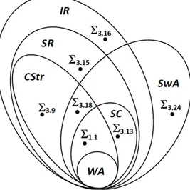
Fig. 3.1. Relationships amongWA, SC, CStr, IR and SwA classes.

Theorem 3.24.SC SwA. 2

Proof. First of all observe that for any TGD r and for any existentially

quan-tiﬁed variable y in r, we have that for all Ri ∈ Π(Out(r, y)) and for all Sj ∈ Π(Move(Σ, Out(r, y))) there is a path Ri → · · · → Sj in prop(Σ), denoting that a (null) value could be propagated by means of universally quantiﬁed variables.

Assume now that there is a TGD r′ (not necessarily distinct from r) such that r′ r. Then, there must be an existentially quantiﬁed variable

z in r′ and a universally quantiﬁed variable x in r such that In(r, x) ⊑

M ove(Σ, Out(r′, z)). From Lemma 3.23 we have that Π(In(r, x))⊆ Π(Move( Σ, Out(r′, z))). Moreover, we also have that for every Ri ∈ Π(In(r, x)) and

for every Sj ∈ Π(Out(r, z)) there is an edge Ri →∗ Sj in prop(Σ). Of course,

we also have that for every Tk∈ Π(Out(r′, z)) there is a path Tk→ · · · → Ri,

as Π(In(rx))⊆ Π(Move(Σ, Out(r′, z))).

Consequently, if there is a cycle in Υ (Σ), then there must be a cycle with a special edge in prop(Σ). This implies that if Σ̸∈ SwA, then Σ ̸∈ SC as well, that isSC ⊆ SwA. The strict containment derives from the fact that there are sets of TGDs, such as Σ3.20 in Example 3.20, which are SwA, but not SC.2

The below corollaries present two minor results which have been also in-dependently achieved in [Mei10].

Corollary 3.25.SwA ∦ CStr. 2

Proof. The set of constraints of Example 3.10 is (c-)stratiﬁed, but not

super-weakly acyclic, thus CStr ̸⊆ SwA. Since SC ̸⊆ CStr and SC SwA, then

(33)

Example 3.26. The following set of constraints Σ3.26 is neither in IR nor in SR but it belongs to the class SwA:

r1: N (x)→ ∃y ∃z E(x, y, z) r2: E(x, y, z)→ T (x, y, z) r3: T (x, y, y)→ N(y)

Indeed, Σ_3.26′ is not IR (and, obviously, SR) since r1 <P r2 <P r3 <P r1,

where P ={E2, E3, T2, T3, N1, E1, T1} and the unique component is not safe

(i.e. N1 →∗ E2, E2 → T2, T2 → N1). Moreover, Σ3.26 is in SwA since the

corresponding trigger graph is acyclic. 2

Corollary 3.27.SwA ∦ SR and SwA ∦ IR. 2

Proof. Straightforward from Examples 3.26 and 3.10. 2

The previous results state that super-weak acyclicity generalizes safety and is not comparable with c-stratiﬁcation and inductive restriction criteria. A complete characterization of the relationships among termination condition criteria is summed up in Figure 3.1. Notice that a set of constraints Σi in