https://doi.org/10.12988/ams.2017.77216
Potential and Limitations of D.E.A. as
a Bankruptcy Prediction Tool in the Light of
a Study on Italian Listed Companies
Silvia CondelloDeloitte & Touche S.p.A., Italy Antonio Del Pozzo
University of Messina, Messina, Italy Salvatore Loprevite
University “Dante Alighieri” of Reggio Calabria Via Del Torrione, 95 - 89125 Reggio Calabria, Italy
Bruno Ricca
University of Messina, Messina, Italy
Copyright © 2017 Silvia Condello et al. This article is distributed under the Creative Commons Attribution License, which permits unrestricted use, distribution, and reproduction in any medium, provided the original work is properly cited.
Abstract*
This paper presents the results of an empirical study carried out on a sample of Italian firms listed on the Stock Exchange and sets out to evaluate the effectiveness of Data Envelopment Analysis (D.E.A.) as a tool for bankruptcy prediction in the short term, as compared to Discriminant Analysis and Logit
Regression. In particular, the research verifies whether, in line with studies
already carried out on samples of firms in other countries, D.E.A. is found to have
*Although the article is the result of joint reflections of all authors, sections 2 and 3.1 are
attributable to Silvia Condello, sections 5 and 6 are attributable to Antonio Del Pozzo, sections 1 and 3.2 are attributable to Salvatore Loprevite; sections 3.3 and 4 are attributable to Bruno Ricca.
a greater capacity for bankruptcy prediction, while Logit Regression and
Discriminant Analysis perform better in non-bankruptcy and overall prediction in
the short term.
Keywords: Default prediction, Additive D.E.A Model, Discriminant Analysis, Logit Regression
1. Introduction
Identifying signs of financial difficulty that may lead to bankruptcy is fundamental in order to intervene early to solve corporate imbalance and save the interests involved before the company default.
Many researchers have looked into the difficult question of identifying the symptoms of corporate financial crises, developing numerous models for
bankruptcy prediction of various kinds and of varying scope.
One essential reference point used for bankruptcy prediction is undoubtedly financial statement values. Indeed, in the literature various default prediction
models have been constructed based on economic-financial data. Ground-breaking
contributions by authors such as Beaver (1966), Altman (1968), Merton (1974), Wilcox (1976) and Damodaran (1996) set out models that have become points of reference in doctrine and the subject of numerous theoretical and empirical studies aimed at testing them and/or improving them. The challenge faced by investors and other stakeholders is that of choosing the most suitable tools for predicting whether a firm is heading towards bankruptcy. Indeed, models able to provide reliable results are not only needed for investors to evaluate investment risk, but can also guide and support management in decision-making (Karimi and Sahlan, 2014). For this reason, academic research is constantly engaged in the development of default prediction models, valid at any time and for any type of business, based on one or more parameters of evaluation of bankruptcy risk. An innovative approach based on economic-financial data which has been used quite recently for evaluating default risk (Premachandra et al., 2009 and 2011; Karimi and Sahlan, 2014) and which shows potential for development is the use of Data Envelopment Analysis (D.E.A.). This is a technique first used in the late 1970s as a tool for comparative study of different productive units and which, over time, has shown itself to be applicable in numerous fields of corporate analysis. In this paper, we present the results of an empirical study carried out on a sample of Italian firms for purposes of verifying the effectiveness of D.E.A. in comparison with Discriminant Analysis and Logit Regression. Comparison of the various models is performed considering their capacity for predicting bankruptcy,
non-bankruptcy and overall capacity, as demonstrated by each model on a
short-term timescale.
The paper is structured as follows.
Section 2 contains an overview of the main literature on default prediction, paying particular attention to recent developments that have led to examination of the potentialities of D.E.A. as a tool for assessment of bankruptcy risk. This section
aims, therefore, to highlight the state of the art in literature and how our paper fits into it. Section 3 sets out in detail the structure of the study: database; research hypothesis, methodology and data analysis models. Section 4 presents the results of the empirical study. Section 5 describes how D.E.A. is used to identify businesses that are inefficient from an economic-financial point of view and underlines the potential for its use in bankruptcy prediction. Section 6 contains the conclusions reached regarding the results obtained from comparison of the three techniques and the comparative advantages and limitations of D.E.A.
2. Theoretical Reference
In economic literature, the topic of corporate bankruptcy has been analysed from many different viewpoints:
bankruptcy prediction (failure prediction or default prediction);
financial difficulty prediction;
credit risk assessment;
early warning systems.
The studies carried out in the various fields listed above have essentially involved empirical models which, unlike theoretical ones, can be used in a more flexible way.
“Traditional models” of bankruptcy prediction, based on economic-financial data, have been developed according to various approaches: univariate, multivariate (Discriminant Analysis, Linear Regression, Logit Regression, Probit), other methods.
Two of the best-known univariate models are those developed by W. Beaver (1966) and A. Damodaran (2002). W. Beaver (1966) came up with the pioneering so-called univariate model, identifying the cash flow/overall debt relationship as the most effective indicator for predicting bankruptcy. From a general viewpoint, his contribution is considered to be significant because it underlined that: a) financial indicators, or accounting data in general, are a useful source of information for early identification of bankruptcy risk; b) not all economic-financial indicators are able to predict bankruptcy with the same degree of accuracy; c) financial indicators are more successful in predicting non-bankruptcy than bankruptcy.
Another important and well-known univariate model is the one developed by A. Damodaran (2002 and 2008), who thought up a rating model based on the interest
coverage ratio (EBIT/Interest expense) (A. Damodaran, 2002 and 2008).
These pioneering models were superseded by the multivariate approach, which considers it necessary to use methods capable of bringing together signals arriving from multiple variables in a composite indicator synthesising a company’s state of health.
Literature on the multivariate approach is dominated by traditional methods of
credit scoring, the principal ones being:
Logit and Probit Regression models;
models from the field of Artificial Intelligence, such as Neural Networks. As regards multivariate models, the main contribution, as we know, was made by E. Altman (1968), reworked in 1977 by E. Altman et al.; these models combine different indicators in a prediction model with the use of Multivariate
Discriminant Analysis1.
Heuristic models have been joined by prediction models based on formal meanings of the concept of bankruptcy. As mentioned above, these theoretical models have had little success when applied practically. J.W. Wilcox (1976) developed a model based on the probability of positive cash flows and on the value of settlement capital available to creditors in the event of default: this study inspired the so-called risk-of-ruin models, put forward later by other researchers (J. Vinso, 1979; J. Scott, 1981; L. Olivotto, 1989, E. Laitinen e T. Laitinen, 1998). The model developed by R. C. Merton (1974), which interprets default through the relationship between the value of operational capital and the value of debt, is also worth mentioning for its theoretical value, even though it has a limited capacity in distinguishing non-bankrupt firms from bankrupt ones.
Numerous empirical and theoretical studies have followed the above-mentioned pioneering contributions, setting out to retest or improve them. We will simply observe that models based on Discriminant Analysis and on Logit Regression are predominant (M.A. Aziz and H.D. Har, 2006), and that the latter seem to be preferable (R. Eisenbeis, 1977; R.A. Collins and R.D. Green, 1982; S. Grice and R. Ingram, 2001). Further bibliographic references on the construction logic of
Discriminant Analysis and Logit Regression will be provided below in section 3.3.
“Traditional” empirical models for evaluating default risk have implementation issues (Premachandra, 2009), because it is necessary to: a) respect numerous assumptions on the distribution of variables and their relationships, as well as on the homogeneity of the variance/covariance matrices among the various groups surveyed; b) estimate the probabilities of observations falling within the various groups and the related costs for Type I and II errors; c) have two samples of significant size (training sample and validation sample). There are also issues concerning prediction performance, because the accuracy of estimates measured on samples declines on different samples (J. Begley et al., 1996).
These limitations have encouraged the search for alternative approaches. One such approach, which has slowly been attracting wider attention in studies, is the application of D.E.A. for bankruptcy prediction.
Cielen, Peeters and Vanhoof (2004) carried out a study aimed at comparing the
1 With a study carried out on equal samples of bankrupt and operational firms, Altman developed
the famous Z-score model, which allows us to distinguish, in relation to various cut-off points, firms subject to bankruptcy, those in operation and those in the so called “ignorance zone” (firms that are classified as in financial distress, but without a well-defined classification and which require further analysis). The model was developed through the linear combination of five financial indicators: a) Working Capital/Total Assets; b) Retained Earnings/Total Assets; c) EBIT/Total Assets; d) Market Value of equity/Book Value of Total Debt); e) Sales/Total Assets.
performance of three different models capable of distinguishing between failing/non-failing firms: a Linear Programming Model, a D.E.A. model and a
Machine-Learning Model (arising from studies on artificial intelligence). The
logic of this paper, which in a certain sense adopts the decision-making perspective of banks, is aimed at minimising possible costs of erroneous
classification of credit towards clients, in order to mitigate the risk of granting
credit that will deteriorate and the risk of not granting credit that will remain in
bonis. The authors concluded that D.E.A. seems to offer better results in terms of
accuracy, costs and clarity of results compared to Linear Programming and the
Machine-Learning model.
Premachandra et al (2009) carried out an empirical study comparing the performance of D.E.A. with that of Logit Regression. The study presents D.E.A. as a non-parametric method easily applicable to the evaluation of corporate bankruptcy. In particular, the authors demonstrated that, while D.E.A. has a lower overall level of correct prediction than Logit Regression, it is a more accurate tool when predicting bankruptcy. The study especially shows that D.E.A. can be achieve good results in predicting bankruptcy even with very large samples characterised by a low value for the relationship between the number of Bankrupt
Firms (BR) and number of Non-Bankrupt Firms (NBR) belonging to the sample. It
is useful to note, moreover, that this contribution, as well as producing results that seem to demonstrate the quality of D.E.A. as a bankruptcy prediction tool, is distinguished by another important innovation regarding data protection method at the frontier of the D.E.A. model. Indeed, the authors put forward a particular approach aimed at using the D.E.A. model to construct a bankruptcy frontier rather than a success frontier, in other words an inefficiency, rather than an efficiency, barrier. Indeed, from a traditional viewpoint, D.E.A. models aim to evaluate the efficiency of the production possibility set, which is measured by the “output/input” ratio, identifying the most efficient Decision Making Units (D.M.U.) as those that maximise said ratio. In their 2009 contribution, on the other hand, Premachandra et al. inverted this logic in order to construct the frontier of a given sample of firms as a bankruptcy frontier, on which bankrupt firms are situated, and a bankruptcy possibility set, which represents the possible bankruptcies of DMUs contained within the frontier.
Premachandra et al. (2011) later carried out a second study in which they performed more sophisticated analysis, based on the calculation of two frontiers (bankruptcy and non-bankruptcy) and of a so called assessment index, in other words an index capable of identifying firms in financial trouble by using a combination of two frontiers (bankruptcy and non-bankruptcy)2. Literature has given preference to the earlier model developed by Premachandra et al. ratherthan
2 In this way, the authors obtained two barriers and two sets of efficiency score, which are scores
identified on the bankruptcy frontier and those identified on the success frontier. Since this method leads to different efficiency scores for individual DMUs and different rates of correct prediction in the two models, the authors introduce the assessment index, in other words a factor that combines the two coefficients obtained taking into account the importance, for the data user, of the bankruptcy prediction or non-bankruptcy prediction information.
the later one, due to its simplicity of use. For the same reason, we will also use the approach adopted by Premachandra et al. in their 2009 study in this paper.
Hampel et al. (2012) applied the D.E.A. method to the evaluation of bankruptcy of agricultural firms, demonstrating a high degree of effectiveness for this model regarding firms in this sector.
Roháčová and Kráľ (2015) used a very similar approach to the one adopted by Premachandra et al. with the intention of demonstrating that D.E.A. is a simple and effective tool for bankruptcy prediction using the technique that allows identification of the Corporate Failure Frontier (CFF), in other words the frontier on which firms about to fail are situated. This study, carried out on a sample of Slovakian firms, set out not only to demonstrate the effectiveness of D.E.A. as a bankruptcy prediction tool, but also to provide some solutions regarding treatment of possible anomalous values in the dataset.
Sueyoshi and Goto (2009) carried out a study comparing the performance of a traditional D.E.A. model with that of a discriminant D.E.A. model, with the aim of evaluating and comparing the strong and weak points of each of the two methodologies. The results of the study showed that additive D.E.A. is a suitable tool for rapid evaluation of bankruptcy risk, while the discriminant D.E.A. model is better suited to evaluating the gradual process of economic-financial distress observed over a specific time period.
3. Research design
3.1 Sample and data
In this section, we describe the process followed in selecting the sample for our survey in reference to the Italian context.
It should first be mentioned that studies putting forward default prediction models developed on an empirical basis must decide the composition of the sample in terms of number of non-bankrupt firms in relation to number of bankrupt firms. In this regard, there is more than one solution. “Traditional” studies have used both equal samples and samples with a higher number of non-bankrupt firms. Studies proposing the application of D.E.A. as a tool for bankruptcy prediction also have differently composed samples, with a preference for using a higher number of
non-bankrupt firms as opposed to bankrupt ones. The solution adopted by
Premachandra et al. in their works (Premachandra et al., 2009 e 2011), which seems to be the most widely recognised and reused by others in research applying
D.E.A. to default prediction, presumes a sample composed of approximately 1 bankrupt firm for every 20 non-bankrupt firms; thus a rate of 5% bankrupt firms
out of the total number of firms selected. In reality, the authors demonstrated (cfr. Premachandra et al., 2009) that D.E.A. performs better on a smaller size sample and with an equal number of bankrupt firms (BR) and non-bankrupt firms (NBR) in the sample, and that it becomes less effective as the size of the sample increases with concurring reduction in the number of Bankrupt Firms (BR)/number of non-Bankrupt Firms (NBR) ratio. The decision to adopt a sample with a low BR/NBR
ratio seems to be related to the need to use a number of subsets that reflects the NBR/BR ratio of the population, as observed on a concrete level, thus constructing
a model directly applicable to the real-life context, with probabilities that a priori coincide with those of the sample without having to make any further adjustments. Considering that this approach has an underlying logic, we will also adopt it in this paper, using a sample made up of about 95% non-bankrupt firms and about 5% bankrupt firms. The set of indicators that we will use for analysis (see section 3.2 below), in line with previous studies testing D.E.A. as a bankruptcy prediction tool, contains an indicator that posits stock market value. For this reason, our sample was chosen from among companies listed on the Milan Stock Exchange. The data were extracted from the AIDA Bureau van Dijk database.
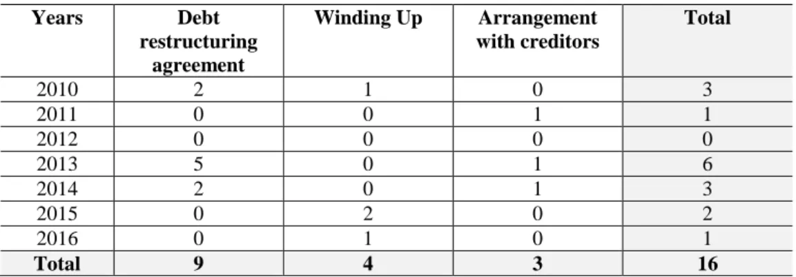
Table 1: Summary of data extracted from AIDA data base
Years Debt restructuring agreement Winding Up Arrangement with creditors Total 2010 2 1 0 3 2011 0 0 1 1 2012 0 0 0 0 2013 5 0 1 6 2014 2 0 1 3 2015 0 2 0 2 2016 0 1 0 1 Total 9 4 3 16
In order to extract the sample, we first verified the number of companies listed on the Stock Exchange that had been subject to bankruptcy procedures had made use of debt restructuring agreements between 01.01.2010 and the date on which the research was carried out, ascertaining that the total number was 16. Table 1 gives an overview of the companies extracted by year and type of procedure.
Based on these data, and in order to be able to carry out a continuity study over at least two accounting periods and with an adequate overall number of firms, we decided to use 2013 and 2014 for reference, with a number of “firms in difficulty” of 6 and 3, respectively. As we were unable to recover the data on stock market capitalisation for one of the firms for the years in question, we took into consideration 8 “firms in difficulty”, 5 of which initiated their procedures in 2013 and three that initiated them in 2014. In order to maintain the above-mentioned ratio of approximately 1 to 20, we composed the following samples for the two years in question:
2013: 101 healthy firms alongside the 5 in difficulty; 2014: 60 healthy firms alongside the 3 in difficulty.
At this point, in order to choose the 101 and the 60 firms for the two years, we: a) extracted from the AIDA database the companies listed on the Stock Exchange with the necessary financial statement values for calculating the indicators to be
used, which AIDA identified as numbering 283; b) eliminated from the list of 283 companies those with missing values and randomly selected the items from the list of the remaining companies.
As we intend to test the prediction capacity of the model at 1 year from the moment of crisis, the accounting data for the two samples were sourced thus: for the first sample, composed of 101 non-bankrupt firms and 5 that went
bankrupt in 2013, we considered the accounting data on 01.01.2012, extracting them from financial statements as of 31.12.2011;
for the second sample, composed of 60 non-bankrupt firms and 3 that went bankrupt in 2014, we considered the accounting data on 01.01.2013, extracting them from financial statements as of 31.12.2012.
The accounting data thus obtained was processed as explained below in the rest of the paper.
3.2 Research hypotheses and economic-financial indicators
As briefly explained above, this paper sets out to test the effectiveness of D.E.A. as a tool for evaluating default risk compared to Discriminant Analysis and Logit
Regression. In particular, by means of analytic comparison of the capacity of the
three models to predict bankruptcy (BR), non-bankruptcy (NBR) and overall (Total Correct Previsions - TCP), this study aims to verify whether, in line with the results already highlighted in the literature, also with reference to the Italian context, D.E.A. demonstrates a lower capacity for TCP prediction compared to
Discriminant Analysis and Logit Regression, but a better level of prediction for Bankrupt Firms (BR).
The following research hypotheses will therefore be tested:
H1: D.E.A. performs worse in overall prediction (TCP) compared to
Discriminant Analysis and Logit Regression;
H2: D.E.A. performs worse in correctly predicting non-bankrupt firms (NBR) compared to Discriminant Analysis and Logit Regression;
H3: while performing worse in overall prediction (TCP) and in NBR prediction, D.E.A. performs better in predicting bankruptcy (BR) compared to the other two models.
As regards the variables, our study uses the same 9 indicators (2 output and 7 input) and follows the same logic in constructing the bankruptcy frontier through
D.E.A. proposed by Premachandra et al. (2009). In particular, as concerns the
logic in constructing the bankruptcy frontier, the input and output variables of the model are chosen thus:
input variables. Financial indicators determined in the form of ratios the
reduction of which expresses situations of greater imbalance or greater
economic-financial tension;
output variables. Financial indicators, also determined in the form of ratios, the increase of which expresses situations of greater vicinity to default.
With this set up, the model will identify firms maximising the ratio between the weighted summation of inputs and that of outputs as those experiencing a situation of greater economic-financial tension and which, therefore, will be positioned on the frontier line. At the same time, the greater the distance of the DMU from the frontier, the lower the chances of bankruptcy in the short term according to the model.
The set of financial variables used is shown in table 2 below. Table 2: Financial variables (output and input)
Output 1 Total Debt/Total Assets (TDTA)
Output 2 Current Liabilities/Total Assets (CLTA)
Input 1 Cash Flow/Total Assets (CFTA)
Input 2 Net Income/Total Assets (NITA)
Input 3 Working Capital/Total Assets (WCTA)
Input 4 Current Assets/Total Assets (CATA)
Input 5 Earnings before interest and taxes/Total assets (EBTA) Input 6 Earnings Before interest and Taxes/Interest Expense
(EBIE)
Input 7 Market Value of Equity/Book Value of Common Equity (MVCE)
3.3 Prediction models
Formulating a prediction means processing knowledge of the past and using a theoretical construction to produce assertions on events yet to happen in order to modify contexts and prospects. In a more formal sense, it can be said that economically this means linking the past with the future (Cipolletta, 1992) using a mathematical model. It is intended, at least, that this analytical formulation should allow economic phenomena to be represented by means of quantitative and/or qualitative variables linked by causal and quantitative relationships, in order to obtain future values to predict possible situations of economic-financial tension. It is clear that the reliability of predictions carried out using a randomly selected sample depends essentially on the choice of variables that constitute the information base and of the mathematical model adopted to represent the economic phenomenon under observation.
Considering the operational context to which this study refers, and with regard to the established aims which should allow evaluation of the default risk of a sample of Italian firms, it was decided to use the multivariate approach to resolve what appears to be a typical classification problem.
On the basis of this choice, the results obtained using Logit Regression (LR) and
Factorial Discriminant Analysis (FDA) will be compared to those from Data Envelopment Analysis (D.E.A.).
the combination of values expressed by the chosen indicators in order to obtain a synthetic measurement that allows us to “discriminate” on the “state of health” of the firms studied. Moreover, the coefficients of the linear function obtained by implementing FDA are equal to those of the regression with ordinary least squares unless there is a constant ratio (Maddala, 1983 and 1992), and in both cases the firms included in the sample are compared to an average firm.
D.E.A., on the other hand, is a non-parametric technique based on mathematical
linear programming allowing us to determine the efficient frontier and bankruptcy
frontier of a group of firms (denominate DMU) characterised by the indicators
chosen. Thus, D.E.A., based on a plurality of inputs and outputs, allows comparison of each individual DMU with the more efficient firms or with the bankrupt ones evaluating, thus, their relative efficiency or inefficiency3.
Logit Regression (Hosmer and Lemeshow, 2000; Agresti, 2002) assumes the
existence of a relationship between the probability of bankruptcy of a firm and a set of indicators (independent variables) linked to the bankruptcy event: in substance, considering the probability of bankruptcy to be a latent variable, we will observe its dichotomous accomplishment4.
Expressed formulaically, the distribution of bankruptcy probability will be:
p = F(ω + ϕI)=∫ 𝑓(ℎ)𝑑ℎ = 1
1+𝑒−(𝜔+ ϕI)
𝜔+ ϕI −∞
in which the logit density function f(h) is: f(h) = 𝑒
ℎ
(1+𝑒ℎ)2
Factorial Discriminant Analysis (Fisher, 1936; Huberty, 1994; Tomassone et al.,
1988) consists in searching for the k-1 linear combinations of q explicative variables that allow us to best separate non-bankrupt firms from bankrupt ones. In this way, we will obtain two internally homogenous and well-separated groups of firms. In substance, FDA searches for a subspace of Rp that minimises the distances between firms belonging to the same group, while maximising those between firms belonging to different groups. Statistically, therefore, the aim is to minimise the inertia within the two groups (non-bankrupt and bankrupt firms), maximising the inertia between said groups.
Thus, based on the assumption that the hypotheses of homoschedasticity of the variance and covariance matrix within the groups, and of multi normality of the explicative variables are valid and defining total inertia V:
V = W + B
where V, W and B are the total, within groups and between groups inertia matrices, respectively.
3 See also section 3.2, infra.
The objective function which will allow us to find the versor5 of the projection axis that maximises the inertia between the groups and minimises the inertia within the groups is given by:
F(u) = 𝑢′𝐵𝑢
𝑢′𝑉𝑢 = max
where u represents the through axis for the centre of gravity of the scatter plot such that the variance of the projected centres of gravity is maximised, while the projection of the variance within the groups is minimised.
The solution is obtained making the derivative of the function F 0 with respect to u in order to get
𝜕𝐹
𝜕𝑢 = 2Bu -2λVu = 0 => V
-1Bu = λu
Thus establishing v = Vu we will have
BV-1v = λv
Thus, the solution lies in searching for the auto-values λ, which represent the inertia quota projected between the groups compared to total inertia, and for the auto-vectors v of the matrix BV-1 , which constitute the discriminant axes, while the auto-vectors uα of matrix B with metric V-1 are defined as discriminant linear
forms.
D.E.A. (Charnes et al., 1978; Cooper at al., 2007) is a non-parametric technique
developed to measure corporate efficiency so as to permit benchmarking analysis among firms, thus to identify an efficient frontier among a group of firms. Premachandra et al. (2009 and 2011) used the non-oriented additive D.E.A. model to identify the inefficiency frontier, in other words to predict bankruptcy situations.
The advantage compared to the two previous econometric/statistical models lies in the fact that no assumptions are required a priori regarding the distribution of the indicators involved in the analysis. Premachandra, in particular, by applying the
non-oriented additive model, proposes an index that allows us to discriminate
between non-bankrupt and bankrupt firms, identifying an efficient frontier that represents non-bankrupt firms and a bankruptcy frontier that represents, on the other hand, bankrupt firms.
This paper uses a non-radial extension6 of the additive model known as Slack
Based Measure of Efficiency-SBM (Tone, 2001). This model will allow us to
5 In mathematics, a versor is a vector in a normalised space of unitary module, used to indicate a
particular direction and course.
6 In D.E.A. models, once the radials are identified, efficiency is measured by applying a
evaluate firms heading for bankruptcy by measuring slack 7 variables independently of the unit of measurement of the variables included in the evaluation. The invariance of the unit of measurement of the variables is guaranteed by the fractionary form of the model (Cooper et al., 2011):
𝑠𝑐𝐼𝑂∗ = 𝑚𝑖𝑛 1 − 1/𝑚 ∑ 𝑠𝑖 − 𝑥𝑖𝑜 𝑚 𝑖=1 1 + 1/𝑠 ∑ 𝑠𝑟 + 𝑦𝑟𝑜 𝑠 𝑟=1
where the score (scIO) represents the efficiency of the firm named DMU0 based on
the summation of the slack variables compared to the inputs or outputs (xo; yo),
under the restraints:
∑ 𝑥𝑖𝑗 λ𝑗 + 𝑠𝑖− = 𝑥𝑖𝑜 𝑛 𝑗=1 𝑖 = 1,2, … , 𝑚 ∑ 𝑦𝑟𝑗 λ𝑗 − 𝑠𝑟+ = 𝑦𝑟𝑜 𝑟 = 1,2, … , 𝑠 𝑛 𝑗=1 λ𝑗, 𝑠𝑖−, 𝑠𝑟+≥ 0∀𝑗, 𝑖, 𝑟
4. Findings
The empirical analysis comparison of the three methods must be viewed in light of the fact that initially, to ensure homogenous treatment, for Logit Regression and Factorial Discriminant Analysis the inverse of the variables identified as “output” in section 3.2 was considered. However, the same variables were discarded a priori since they proved to be statistically insignificant for the purpose of analysis. In conclusion, therefore, only the indicators identified as “input” were used for the above-mentioned analyses. The “output” ratios were added, however, for the D.E.A. analysis.
As explained above, the underlying idea of the logit model is the assumption that there is a relationship between the probability that a firm will default (unobservable variable) and a series of observable measures that are closely tied to the “bankruptcy” event. What is observed in reality, therefore, is not the
efficient frontier. While this has the advantage of expressing efficiency in values between 0 and 1, the disadvantage is that it is impossible to capture the inefficiency of the combination of factors of production and products. This inefficiency can be identified using the Slack Based Measure-SBM version. The SBM D.E.A. model is defined as non-radial and bases its efficiency evaluations on measurement and evaluation of slack.
7 Slack variables represent the gap between individual inputs and outputs and the efficient
probability of bankruptcy (which can be considered a latent variable) but a dichotomous accomplishment (0-1) of such a probability.
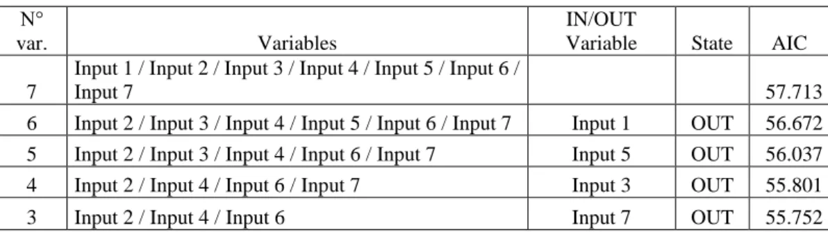
The variables included in the model were selected using the backward stepwise method8:
Table 3: Stepwise procedure for selection of variables
N°
var. Variables
IN/OUT
Variable State AIC
7
Input 1 / Input 2 / Input 3 / Input 4 / Input 5 / Input 6 /
Input 7 57.713
6 Input 2 / Input 3 / Input 4 / Input 5 / Input 6 / Input 7 Input 1 OUT 56.672 5 Input 2 / Input 3 / Input 4 / Input 6 / Input 7 Input 5 OUT 56.037
4 Input 2 / Input 4 / Input 6 / Input 7 Input 3 OUT 55.801
3 Input 2 / Input 4 / Input 6 Input 7 OUT 55.752
Parameters were estimated using the most similarity method, obtaining:
Table 4: Estimate of parameters
Source Value Standard error Wald Chi-squared Pr >
Chi² Odds ratio
Odds ratio Lower limit (95%) Odds ratio Upper limit (95%) Intercetta -2.265 0.969 5.466 0.019 Input 2 -11.016 3.232 11.615 0.001 0.000 0.000 0.009 Input 4 -5.332 3.035 3.086 0.079 0.005 0.000 1.853 Input 6 0.017 0.008 4.547 0.033 1.017 1.001 1.033
From which we deduce the equation of the model:
Prev(STATUS) = 1 / (1 + exp(-(-2,26 -11,01*Input 2 -5,33*Input 4 +0,01*Input 6)))
8 Backward selection means that the equation initially includes all the independent variables and
that at each stage the variable that does not contribute sufficiently to explaining the dependent variable. Once the variable leaves the equation it cannot come back in. In this case the selection method is based on Akaike's information criterion, indicated as AIC, which is a method for evaluating and comparing statistical models developed by the Japanese mathematician H. Akaike and presented to the mathematics community in 1974. It measures the quality of an estimate of a statistical model, taking into account both the how well the model adapts and its complexity. It is based on the concept of information entropy and offers a relative measurement of the information lost when a given model is used to describe reality. The rule is preference for models with the lowest AIC.
From the χ2 test applied to the Hosmer-Lemeshow test9 we can assert that the
model explains the data well:
Table 5: Hosmer-Lemeshow Test
Statistical Test Chi-squared GDL Pr > Chi²
Hosmer-Lemeshow Test 6.223 8 0.622
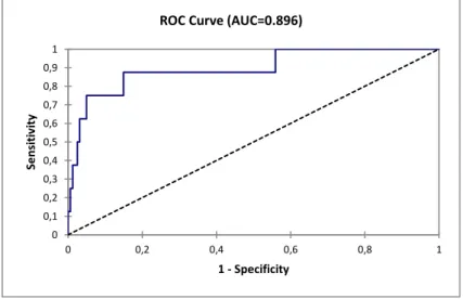
Moreover, the area under the ROC curve10 (AUC = 0.896) allows to assert that the performance of the model is good.
Observing the parameters of the equation and the Odds Ratio we can see that, if other variables in the equation remain constant, when a unit of ratio Input 2 or
Input 4 increases, the probability of bankruptcy decreases, whereas it increases if
a unit of the ratio Input 6 increases. In conclusion, with Logit Regression it is possible to estimate the predictions of the dependent variable allowing us to obtain the following result:
9 The Hosmer-Lemeshow test is a statistical test that allows evaluation of the adaptability for Logit
Regression. The test is carried out by dividing the population into percentiles and calculating the
number of expected and observed events for each percentile. Comparison is made using the χ2 test, which permits determination of whether the difference between the expected and observed events is statistically insignificant.
10 The ROC curve is used to evaluate the performance of the model by grouping together the area
under the curve (AUC). The area under the curve (AUC) is a synthetic index calculated for ROC curves. The AUC is the probability that a positive event is classified as positive by the test in all possible values of the test. For an ideal model we would have AUC = 1. A model is usually considered good when the value of the AUC is greater than 0.7. A model with good discriminant capacity should have an AUC between 0.87 e 0.9. A model with an AUC above 0.9 is excellent.
0 0,1 0,2 0,3 0,4 0,5 0,6 0,7 0,8 0,9 1 0 0,2 0,4 0,6 0,8 1 Se ns it iv it y 1 - Specificity
Table 6: Correct predictions Logit Regression
Logit Regression
P(PBR/BR) 25.00%
P(PNBR/NBR) 99.38%
TOTCORRPRED 95.86%
The results obtained using Logit Regression were compared to those obtained from Factorial Discriminant Analysis.
As explained in the previous section, Factorial Discriminant Analysis permits us to identify the discriminant axes and the discriminant linear form that allows the distinction between non-bankrupt firms and bankrupt ones.
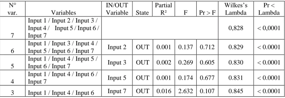
In this case, the backward stepwise11 method was used to select significant variables to be included in the model and those to be removed based on their value in the “Wilks’s lambda” 12 test or the “F test”.13
Table 7: Stepwise procedure for selection of variables
N° var. Variables IN/OUT Variable State Partial R² F Pr > F Wilkes’s Lambda Pr < Lambda 7
Input 1 / Input 2 / Input 3 / Input 4 / Input 5 / Input 6 / Input 7
0,828 < 0,0001
6
Input 1 / Input 3 / Input 4 /
Input 5 / Input 6 / Input 7 Input 2 OUT 0.001 0.137 0.712 0.829 < 0.0001
5
Input 1 / Input 4 / Input 5 /
Input 6 / Input 7 Input 3 OUT 0.002 0.269 0.605 0.830 < 0.0001
4
Input 1 / Input 4 / Input 6 /
Input 7 Input 5 OUT 0.001 0.174 0.677 0.831 < 0.0001
3 Input 1 / Input 4 / Input 6 Input 7 OUT 0.016 2.632 0.107 0.845 < 0.0001
The table below shows the discriminant functions that, in this case, will be linear. Indeed, as a fundamental hypothesis it was decided to consider the intra-class covariance matrices of the two groups of firms as being equal.
11 The stepwise methodology is used to estimate multivariate models when there are numerous
variables. It fulfils the need to select an “optimal” subset among a larger number of explicative variables for the construction of an efficient model.
12 A multivariate test to evaluate the hypothesis that two or more groups originate from
populations with the same median, also known as U statistic. High values indicate that the group medians are not very different (equal to 1 if the medians are all equal). Low values indicate differences in the group medians.
13 The F test values come from the ANOVA calculated on each individual variable. The value of F
and the significance gives us further information on the difference between the groups. When F is high and the level of significance is sufficiently low (between 0.01 and 0.05), the null hypothesis can be rejected. In other words, a low level of significance indicates that the results observed in the sample do not depend on the case and, thus, it is right to expect them to be equal in the population.
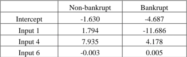
Table 8: Estimate of parameters Non-bankrupt Bankrupt Intercept -1.630 -4.687 Input 1 1.794 -11.686 Input 4 7.935 4.178 Input 6 -0.003 0.005
Thus, the cut off will be at 3.057 and the linear discriminant function will be: Z = -13.480 input1 -3.757 input4 +0.008 input6
The individual firms will be allocated to the “non-bankrupt” or “bankrupt” group corresponding to the function that shows the highest value. We will thus obtain the probability of belonging to the “non-bankrupt” and “bankrupt” group of firms and the relative (Mahalanobis)14 distance of each individual firm from the centre of gravity of the group to which it has been allocated.
Finally, as in the case of Logit Regression, the area under the ROC10 curve allows us to consider the discriminatory capacity of the model to be good.
The results obtained using Factorial Discriminant Analysis are displayed in table 9:
14 The Mahalanobis distance is a measurement of distance introduced by P.C. Mahalanobis in
1936. It is based on the correlations among variables through which different patterns can be identified and analysed. It is a useful way of determining the similarity of an unknown sample space to a known one. It is different from the Euclidean distance because it takes into account the correlations within the dataset.
0 0,1 0,2 0,3 0,4 0,5 0,6 0,7 0,8 0,9 1 0 0,2 0,4 0,6 0,8 1 Se ns it iv it y 1 - Specificity
Table 9: Correct predictions Discriminant Analysis
Discriminant Analysis
P(PBR/BR) 12.50%
P(PNBR/NBR) 98.76%
TOTCORRPRED 94.67%
For the D.E.A. model, as explained above, seven input indicators and two output indicators were used. The choice of variables was carried out considering that lower input indicator values correspond to a greater probability of corporate bankruptcy. On the other hand, a greater probability of bankruptcy corresponds to higher output indicator values.
In this case, therefore, D.E.A is used to identify the bankruptcy frontier, and the performance of a firm is calculated by comparing its “inefficiency” with the worst performance observed in the dataset under study.
Generally, D.E.A.15 attributes a virtual weight to each firm and the performance
of each individual firm is calculated using a process of linear optimisation, which allows the “inefficiency” ratio to be maximised, finding the best set of weights for each DMU.
The bankruptcy frontier was estimated using the non-oriented SBM (Slack Based
Measured) model under the hypothesis variable returns to scale. The model
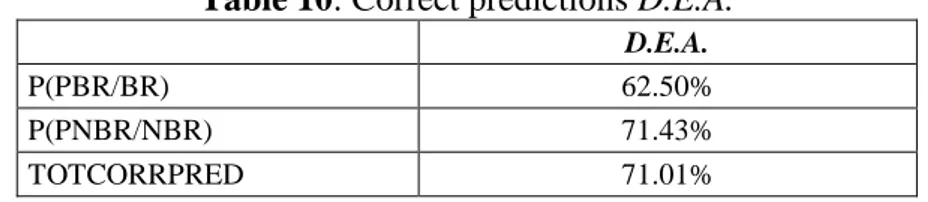
allowed us to identify the scores for each firm with the following results: Table 10: Correct predictions D.E.A.
D.E.A.
P(PBR/BR) 62.50%
P(PNBR/NBR) 71.43%
TOTCORRPRED 71.01%
Table 11 summarises the results obtained from applying the three analysis models. Table 11: Summary of correct predictions of the three models
Discriminant Analysis Logit Regression D.E.A. BR 1 2 5 NBR 159 160 115 P(PBR/BR) 12.50% 25.00% 62.50% P(PNBR/NBR) 98.76% 99.38% 71.43% TOTCORRPRED 94.67% 95.86% 71.01%
As can be seen from the summary of results, Logit Regression is the model that achieves the best TCP performance. The prediction results obtained by this model
15 Data processing was carried out using OSDEA (open source software licensed under GPL3)
are very similar to those obtained using Discriminant Analysis. Both models perform very well in non-bankruptcy prediction in the short term, but prove to be inadequate in predicting bankruptcy over the same time horizon. D.E.A., on the other hand, has lower prediction rates for non-bankrupt firms (NBR), but shows itself to be a tool capable of correctly identifying a larger number of firms that go bankrupt within a year (correct BPR predictions). This is the case even though on our sample the rate of correct PBR predictions is lower than that achieved in previous studies carried out with reference to different territorial contexts.
5. Additional reflections on D.E.A. as a method for bankruptcy
prediction
D.E.A. is a method that allows us to break up the overall performance of a firm
and compare this performance to the optimal one inferred from a sample of firms. It is useful, therefore, for identifying a frontier of efficient firms.
Premachandra used this method to identify the frontier of less efficient firms and tested the ratios between inefficient and bankrupt firms.
The potential of D.E.A. appears to be particularly interesting from an economic-corporate viewpoint because this method allows us to identify a link between the capacity of the firm (its efficiency or inefficiency, as the case may be) and its bankruptcy.
Simulations carried out using the various prediction models show us, in particular, that:
Discriminant Analysis on 8 bankrupt firms considers only 1 as potentially
bankrupt (12.50% correct BR prediction rate), but considers as potentially bankrupt only 2 of the non-bankrupt ones (1.24% of the non-bankrupt firms). Overall, this method predicts 3 bankrupt firms out of a total of 169 (just 1.78%) in the sample, significantly narrowing the bankruptcy area; Logit Regression considers only 2 firms potentially bankrupt out of the 8
bankrupt ones (25.00% correct BR prediction rate), but considers only 1 of the non-bankrupt firms as potentially bankrupt (0.62% of the non-bankrupt firms). Overall, this method predicts 3 bankrupt firms out of a total of 169 (just 1.78%) in the sample, significantly narrowing (even more than
Discriminant Analysis) the bankruptcy area;
D.E.A., considers 5 firms as potentially bankrupt out of the 8 bankrupt ones
(62.50% correct BR prediction rate), but considers 46 of the non-bankrupt firms as potentially bankrupt (28.57% of the non-bankrupt firms). Overall, this method predicts 51 bankrupt firms out of a total of 169, thus 30.18% of the sample, very significantly widening the bankruptcy area.
Authors that have dealt with this topic have deduced the superiority of D.E.A. for the purpose of predicting bankruptcy. In reality, while it is true that D.E.A. identifies 5 bankrupt firms out of 8 within a year (62.50%), it is also true that this method has a low rate of correct prediction for non-bankrupt firms (71.43%), with
a corresponding rate of 28.57% of incorrect predictions, that is to say of non-bankrupt firms that are placed on the bankruptcy barrier.
Due to the significant differences in the results obtained using the various methods, it was decided to examine the later financial statements of the firms identified as inefficient by D.E.A. Over the following 2 years, 47.83% of the firms identified as inefficient resorted to capital increase of debt restructuring procedures.
On the one hand, this empirical evidence confirms the great potential of D.E.A. as a tool for analysing economic-financial efficiency/inefficiency; on the other hand, it confirms that bankruptcy is conditioned by decisions of shareholders not to abandon the firm to its fate or to involve creditors in corporate restructuring appealing to so-called bankruptcy costs. This further study carried out on the two years following placement on the bankruptcy barrier for firms identified as potentially bankrupt by D.E.A. lets us realise that, in any case, this method selected a substantial percentage of the firms at greatest risk.
6. Conclusions
In this paper, a comparison was made between the prediction capacity of various bankruptcy prediction methods. Particularly, the capacity of D.E.A. for identifying the firms most likely to fail was tested, in comparison with the capacity of
Discriminant Analysis and Logit Regression methods.
The methods were tested on a sample of Italian firms listed on the Stock Exchange using the same input and output indicators as Premachandra et al. (2009).
The results confirm what had already been found in literature16 with reference to
different contexts, although in our work, in reference to the Italian context for
D.E.A., lower rates of correct bankruptcy prediction [P(PBR/BR)] and overall
prediction TOTCORRPRED were found in comparison with those found by other authors for D.E.A. with reference to other territorial contexts. It can therefore be said that the analysis confirms the three research hypotheses:
H1: D.E.A. shows a lower overall performance (TCP) compared to the Logit
Regression and Discriminant Analysis;
H2: D.E.A. shows a lower performance in correctly predicting non-bankrupt firms (NBR) compared to the Logit Regression and Discriminant Analysis; H3: despite lower rates of correct overall predictions (TCP) and relative to
NBR, D.E.A. shows a better bankruptcy prediction performance (BR) compared to the other two models.
D.E.A. significantly broadens the area of inefficient and thus potentially bankrupt
firms, which evidently leads to a higher likelihood of selecting the firms that actually end up bankrupt. This, however, produces the unwanted effect of consi-
dering many firms that actually carry on operating regularly as potentially bankrupt.
The difference in data encouraged us to verify the subsequent events of the firms considered to be at risk. Such further analysis led to the discovery that, over the following two years, 47% of the firms deemed to be inefficient resorted to capital increase or debt restructuring procedures.
Such results prove, with reference to the examined context, not only that D.E.A. cannot be considered a method equipped with a superior overall prediction capacity in comparison to the other techniques, but also that it is a tool that significantly broadens bankruptcy prediction, from a perspective we could describe as prudential.
Therefore, to promote an effective use of D.E.A. as a tool for the assessment of default risk, a multi-phase process that makes use of D.E.A. as a tool for bankruptcy prediction should be considered; subsequently, we should consider another tool of analysis to further discriminate the non-bankrupt firms among those identified by D.E.A. as potentially bankrupt.
References
[1] A. Agresti, Categorical Data Analysis, 2nd Edition, John Wiley and Sons, New York, 2002. https://doi.org/10.1002/0471249688
[2] E.I. Altman, Financial Ratios, Discriminant Analysis and the Prediction of Corporate Bankruptcy, Journal of Finance, 23 (1968), no. 4, 589 - 609. https://doi.org/10.2307/2978933
[3] E.I. Altman, Predicting Railroad Bankruptcies in America, Bell Journal of
Economics and Management Science, 4 (1973), no. 1, 184 -211.
https://doi.org/10.2307/3003144
[4] E.I. Altman, Measuring Corporate Bond Mortality and Performance, Journal
of Finance, 44 (1989), no. 4, 909 - 922.
https://doi.org/10.1111/j.1540-6261.1989.tb02630.x
[5] E.I. Altman, Corporate Financial Distress and Bankruptcy, 2nd Ed., Wiley, New York, 1993.
[6] W.H. Beaver, Financial ratios as predictors of failures, Journal of Accounting
Research, 4 (1966), 71 - 111. https://doi.org/10.2307/2490171
[7] W.H. Beaver, Market prices, financial ratios and the prediction of failure,
Journal of Accounting Research, 6 (1968), 179 - 192.
[8] A. Charnes, W.W. Cooper and E. Rhodes, Measuring the efficiency of decision making units, European Journal of Operational Research, 2 (1978), 429 - 444. https://doi.org/10.1016/0377-2217(78)90138-8
[9] I. Cipolletta, Congiuntura Economica e Previsione. Il Mulino, Bologna, 1992.
[10] W.W. Cooper, L.M. Seiford and K. Tone, Data Envelopment Analysis - A
Comprehensive Text with Models, Applications, References and DEA-Solver Software, 2nd Ed., Springer, 2007.
https://doi.org/10.1007/978-0-387-45283-8
[11] W.W. Cooper, L.M. Seiford and J. Zhu, Handbook on Data Envelopment
Analysis, International Series in Operations Research & Management
Science, Vol. 164, 2nd Ed., Springer, 2011. https://doi.org/10.1007/978-1-4419-6151-8
[12] A. Damodaran, Manuale di Valutazione Finanziaria, McGraw-Hill, Milano, 1996.
[13] A. Damodaran, Investment Valuation, 2nd Ed., John Wiley & Sons, New York, 2002.
[14] A. Damodaran, Strategic Risk Taking, Wharton School Publishing, Philadelphia, 2008.
[15] A. Damodaran, Valutazione delle Aziende, Edizione italiana a cura di Costanza Consolandi, Apogeo, Milano, 2010.
[16] R.A. Fisher, The use of multiple measurements in taxonomic problems,
Annals of Eugenics, 7 (1936), 179 - 188.
https://doi.org/10.1111/j.1469-1809.1936.tb02137.x
[17] D. Hampel, J. Janova and J. Vavřina, DEA as a tool for bankruptcy assessment: the agribusiness case study, Acta Universitatis Agriculturae et
Silviculturae Mendelianae Brunensis, LXI (2012), no. 4, 1177-1182.
[18] D.W. Hosmer and S. Lemeshow, Applied Logistic Regression, 2nd Ed., John Wiley and Sons, New York, 2000. https://doi.org/10.1002/0471722146 [19] C.J. Huberty, Applied Discriminant Analysis, Wiley-Interscience, New York,
1994.
[20] P. Karimi and S.S. Sahlan, A Comparative Assessment of Bankruptcy of the Companies Listed in Tehran Stock Exchange Based on DEA-Additive and
DEA–DA, International Journal of Scientific Management and Development, 2 (2014), no. 11, 578 - 587.
[21] E.K. Laitinen and T. Laitinen, Misclassification in bankruptcy prediction in Finland: human information processing approach, Accounting, Auditing &
Accountability Journal, 11 (1998), no. 2, 216 - 244.
https://doi.org/10.1108/09513579810215509
[22] G.S. Maddala, Limited-Dependent and Qualitative Variables in Econometrics, Cambridge Univ. Press, Cambridge, 1983.
https://doi.org/10.1017/cbo9780511810176
[23] G.S. Maddala, Introduction to Econometrics, 2nd Ed., ed. MacMillan, New York, 1992.
[24] P.C. Mahalanobis, On the Generalized Distance in Statistics, Proceedings of
the National Institute of Science of India, 2 (1936), 49 - 55.
[25] R.C. Merton, On the pricing of corporate debt: the risk structure of interest rates, Journal of Finance, 29 (1974), 449 - 470.
https://doi.org/10.1111/j.1540-6261.1974.tb03058.x
[26] L. Olivotto, La previsione dell’insolvenza d’impresa mediante modelli probabilistici, Finanza, Imprese e Mercati, 1 (1989).
[27] I.M. Premachandra, G.S. Bhabra and T. Sueyoshi, DEA as a tool for bankruptcy assessment: a comparative study with logistic regression technique, European Journal of Operational Research, 193 (2009), 412 - 424. https://doi.org/10.1016/j.ejor.2007.11.036
[28] I.M. Premachandra, Y. Chen and J. Watson, DEA as a tool for predicting corporate failure and success: a case of bankruptcy assessment, Omega, 39 (2011), 620 - 626. https://doi.org/10.1016/j.omega.2011.01.002
[29] V. Roháčová and P. Kráľ, Corporate failure prediction using dea: an application to companies in the Slovak Republic, 18th AMSE Application of Mathematics and Statistics in Economics, Jindřichŭv Hradec, (2015).
[30] J. Scott, The probability of bankruptcy, Journal of Banking and Finance, 5 (1981), 317 - 344. https://doi.org/10.1016/0378-4266(81)90029-7
[31] T. Sueyoshi and M. Goto, DEA–DA for bankruptcy-based performance assessment: Misclassification analysis of Japanese construction industry,
European Journal of Operational Research, 199 (2009), no. 2, 576 - 594.
[32] K. Tone, A slack-based measure of efficiency in data envelopment analysis,
European Journal of Operational Research, 130 (2001), 498 - 509.
https://doi.org/10.1016/s0377-2217(99)00407-5
[33] R. Tomassone, M. Danzart, J.J. Daudin and J. P. Masson, Discrimination et
Classement, Masson, Paris, 1988.
[34] J.D. Vinso, A determination of the Risk of Ruin, The Journal of Financial
and Quantitative Analysis, 14 (1979), no. 1, 77 - 100.
https://doi.org/10.2307/2330656
[35] J.W. Wilcox, The gambler’s ruin approach to business risk, Sloan
Management Review, 18 (1976), no. 1, 33 - 41.