UNIVERSIT `
A DEGLI STUDI DI CATANIA
Dipartimento di Ingegneria Elettrica Elettronica e Informatica
Ph.D. Course in Systems Engineering (XXVIII cycle)
Ph.D. Thesis
MODELING SOLAR RADIATION AND WIND
SPEED TIME SERIES FOR RENEWABLE ENERGY
APPLICATIONS
Silvia Nunnari
Tutors: Prof. Luigi Fortuna Prof. Giorgio Guariso Coordinator: Prof. Luigi Fortuna
To my parents
Life is a mystery, discover it. Mother Teresa
VI
The problem of predicting weather variables, such as solar radi-ation and wind speed, is of great interest for integrating renewable energies plants, into the electric grid. Indeed, since renewable en-ergy sources are intermittent in nature, predicting future values is important to allow the grid to dispatching generators, in order to satisfy the demand. There are essentially two ways to address the issue of weather variables prediction. One is by using Numerical Weather Forecasting (NWF) models, which are reliable, but also quite complex and requires real time information, usually avail-able from Meteorological Agencies only. Furthermore, very powerful computers are required to solve the differential equations involved. The other kinds of methods are represented by the so-called statis-tical modeling approaches, which are based on the use of past data recorded at the site of interest. These latter kinds of methods, com-pared to the former ones, require less computational efforts, but are appropriate only for short time horizons.
This PhD Thesis was devoted to study short-term prediction mod-els for solar radiation and wind speed time series and assessing their performance in the range [1, 24] hours.
It was also studied the predictability of the daily average values, which for obvious reasons, is much more difficult than that of pre-dicting the hourly averages. To mitigate, as far as possible, the difficulties, the prediction was reformulated in terms of a classifica-tion problem. In such a way, instead of predicting 1-day ahead the average value, the target was to predict the class. In this framework, of course, the prediction is as far difficult as large is the number of considered classes. The accuracy of 1-day ahead prediction models of the wind speed class was studied, for various frameworks.
VII
The structure of the Thesis is the following. Some background about solar radiation and wind speed energy is presented in Chap. 1. Anal-ysis of solar radiation and wind speed time series, recorded in differ-ent areas are presdiffer-ented in Chap. 2 and 3, respectively. Some litera-ture references dealing with techniques for modeling wind speed and solar radiation time series are given in Chap. 4, focusing essentially on NAR (Nonlinear Auto Regressive) and EPS (Embedded Phase Space) models, since are the ones considered in this work. Results obtained by modeling solar radiation and wind speed time series are reported in Chap. 5 and 6 respectively. Clustering approaches of daily pattern of solar radiation and wind speed time series are given in Chap 7 and 8, respectively, while concluding remarks are sketched in Chap. 9.
Contents
1 Background . . . 1
1.1 Energy from the Sun . . . 1
1.2 Energy from the Wind . . . 4
1.3 Conclusions . . . 8
2 Analysis of Solar Radiation Time Series . . . 11
2.1 Stationarity Analysis . . . 12
2.2 Space-time plots . . . 14
2.3 Autocorrelation and Mutual Information . . . 15
2.4 Power Spectra . . . 17
2.5 Hurst Exponent and Fractal dimension . . . 18
2.6 Multifractal spectrum of solar radiation . . . 19
2.7 Estimation of the embedding dimension . . . 23
2.8 Maximal Lyapunov exponent . . . 24
2.9 Conclusions . . . 24
3 Analysis of Wind Speed Time Series . . . 27
X Contents
3.2 Autocorrelation and Mutual Information . . . 29
3.3 Power Spectra . . . 31
3.4 Hurst Exponent and Fractal dimension . . . 33
3.5 Multifractal Spectrum . . . 34
3.6 Estimation of the embedding dimension . . . 39
3.7 Maximal Lyapunov exponent . . . 40
3.8 Conclusions . . . 40
4 Time series models for wind speed and solar radiation . . . 43
4.1 NAR and EPS time series models . . . 44
4.2 Multi-step ahead prediction models . . . 47
4.3 Mapping approximation . . . 47
4.3.1 The Neuro Fuzzy approach . . . 48
4.3.2 The FeedForward Neural Network Approach . . . 49
4.4 Conclusions . . . 49
5 Modeling hourly average solar radiation time series 51 5.1 Performances of the NARX Neuro-Fuzzy modeling approach . . . 51
5.2 Performances of the NARNF approach . . . 56
5.3 Performances of the EPS Neuro-Fuzzy modeling approach . . . 58
5.4 Performances of the EPSNF approach . . . 60
5.5 Performances of the NARNN approach . . . 63
5.6 A direct comparison between the EPSNF and EPSNN approaches . . . 65
Contents XI
6 Modeling hourly average wind speed time series . . 69
6.1 Performances of the NARNF approach . . . 69
6.2 Performances of the ARX and NARX NN approach . 76 6.3 Performances of the EPS approach . . . 79
6.3.1 Performances of the EPSNF approach . . . 79
6.3.2 Performances of the EPSNN approach . . . 82
6.4 A direct comparison among NARX and EPS models . 82 6.5 Conclusions . . . 82
7 Clustering Daily Solar Radiation Time Series . . . 85
7.1 Problem statement . . . 86
7.2 The area ratio Ar index . . . 88
7.3 The I index . . . 90
7.4 The proposed classification strategy . . . 92
7.5 Numerical Results . . . 94
7.6 Conclusions . . . 98
8 Clustering Daily Wind Speed Time Series . . . 99
8.1 Introduction . . . 99
8.2 Two features of daily wind speed time series . . . 101
8.3 The Wr index . . . 101
8.4 The Hurst exponent of daily wind speed . . . 103
8.5 Wind speed time series classification . . . 103
8.6 Some applications . . . 106
8.7 Predicting the class . . . 108
8.8 Identify NAR models for Wr(d) and H(d) . . . 108
8.9 Assessing the performance . . . 111
XII Contents
9 Concluding remarks . . . 117 10 Acknowledgements . . . 121 References . . . 123
1
Background
Several form of alternative sources of energy are present in nature almost in unlimited quantities, referred to as renewable, since are continuously regenerated. The main renewable sources are based on solar energy, on thermal energy contained in the Earth interior and on gravitational energy. From the Sun naturally derives accu-mulations of water to produce hydroelectric power, wind for aeolic turbine generators, electric energy by photovoltaics plants and solar thermal. Furthermore from the photosynthesis process it is possi-ble to derive energy from biomass. The following sections focuses essentially on solar radiation and wind speed energy, since are the ones considered in this work. Most of information reported in this chapter refers to [1] and [2].
1.1 Energy from the Sun
The Sun is certainly the main source of renewable energy. Just to have an idea it is possible to say that the Sun delivers towards the surface of the terrestrial hemisphere exposed a power exceeding 50
2 1 Background
thousand Tera Watt which is about 10 thousand times the energy used all over the world [1]. A part of this energy reaches the outer part of the Earths atmosphere with an average irradiance of about 1367 W/m2
, a value which varies as a function of the Earth-to-Sun distance and of the solar activity (sunspots). The problem of estimating the average hourly global solar radiation I(h, d), for any hour h of a day d of the year, at any site, has been addressed in literature by several authors such as [3]. It depends on a quite large number of parameters which, roughly speaking, can be summarized as follows: the distance from the sun, the duration of the daily sunlight period, the inclinations of solar rays to the horizon, the transparency of the atmosphere towards heat radiation and the output of solar radiation. Some of these factors are connected with mechanical parameters which describes the revolution of Earth around the Sun and on the Earth spinning about itself. Others factors depend on the properties of the atmosphere and are stochastic in nature, such as the cloud cover features (size, speed and number) and the degree of pollution.
The average annual irradance in European Countries is shown in Figure 1.1. In particular in Italy the average annual irradiance varies from 3.6 KW h/m2
a day of the Po Valley to the 4.7 KW h/m2
a day in the South and Centre and to the 5.4 KW h/m2 a day of Sicily. When passing through the atmosphere, the solar radiation decreases in intensity because it is partially reflected and absorbed (above all by the water vapor and by the other atmospheric gases). The radiation which passes through is partially diffused by the air and by the solid particles suspended in the air, as shown in Figure 1.2. Therefore the radiation falling on a
1.1 Energy from the Sun 3
Fig. 1.1.Solar Radiation in Europe
4 1 Background
horizontal surface is constituted by a direct radiation, associated to the direct irradiance on the surface, by a diffuse radiation which strikes the surface from the whole sky and not from a specific part of it and by a radiation reflected on a given surface by the ground and by the surrounding environment. In winter the sky is overcast and the diffuse component is greater than the direct one.
1.2 Energy from the Wind
The Earth continuously releases into the atmosphere the heat ceived by the sun, but unevenly. In the areas where less heat is re-leased (cool air zones) the pressure of atmospheric gases increases, whereas where more heat is released, air warms up and gas pres-sure decreases. As a consequence, a macro-circulation due to the convective motions is created as shown in Figure 1.3. Air masses get warm, reduce their density and rise, thus drawing cooler air flowing over the earth surface. This motion of warm and cool air masses generates high pressure and low pressure areas permanently present in the atmosphere and also influenced by the rotation of the earth. Since the atmosphere tends to constantly re-establish the pressure balance, the air moves from the areas where the pres-sure is higher towards those where it is lower; therefore, wind is the movement of an air mass, more or less quick, between zones at different pressure. The greater the pressure difference, the quicker the air flow and consequently the stronger the wind. In reality, the wind does not blow in the direction joining the center of the high pressure with that of the low pressure, but in the northern
hemi-1.2 Energy from the Wind 5
Fig. 1.3.Air mass circulation due to Solar Radiation.
sphere it veers to the right, circulating around the high pressure centers with clockwise rotation and around the low pressure ones in the opposite direction. In the practice, who keeps his back to the wind has on his left the low pressure area B and on his right the high pressure area A, as shown in Figure 1.4. In the southern hemisphere the opposite occurs.
On a large scale, at different latitudes, a circulation of air masses can be noticed, which is cyclically influenced by the seasons. On a smaller scale, there is a different heating between the dry land and the water masses, with the consequent formation of the daily sea and earth breezes. The profile and unevenness of the surface of the dry land or of the sea deeply affect the wind and its local charac-teristics; in fact the wind blows with higher intensity on large and flat surfaces, such as the sea: this represents the main element of
6 1 Background
Fig. 1.4.Wind rotation around high and low pressure centers.
interest for wind plants on-and off shore. Moreover, the wind gets stronger on the top of the rises or in the valleys oriented parallel to the direction of the dominant wind, whereas it slows down on uneven surfaces, such as towns or forests, and its speed with re-spect to the height above ground is influenced by the conditions of atmospheric stability.
The average wind speed in Italy, measured at 25 m a.s.l., ranges from 6−7 m/s from the South Eastern to the 3 m/s of the Northern part of Italy, but the largest areas are featured by 4 − 5 and 5 − 6. m/s, as shown in Figure 1.5. In order to exploit wind energy, it is very important to take into account the strong speed variations between different places: sites separated by few kilometers may be subject to very different wind conditions and have different impli-cation for the installation purposes of wind turbines. The strength of the wind changes on a daily, hour or minute scale, according
1.2 Energy from the Wind 7
Fig. 1.5. Average wind speed map in m/s in Italy as results from http://atlanteeolico.rse-web.it/viewer.htm.
to the weather conditions. Moreover, the direction and intensity of the wind fluctuate rapidly around the average value: it is the tur-bulence, which represents an important characteristic of wind since it causes fluctuations of the strength exerted on the blades of the turbines, thus increasing wear and tear and reducing their mean life. On complex terrain, the turbulence level may vary between 15% and 20%, whereas in open sea this value can be comprised in the range from 10% to 14%. Variability and uncertainty of winds
8 1 Background
represent the main disadvantages of the electrical energy derived from the wind source. In fact, as far as the amount of power pro-duced by the wind plant is small in comparison with the size of the grid to which it is connected, the variability of energy production from wind source does not destabilize the grid itself and can be considered as a change in the demand for conventional generators. Instead, in some countries, large-size wind plants are being con-sidered, prevailingly offshore groups of turbines. Such wind farms shall have a power of hundreds of MW, equivalent to that of conven-tional plants, and therefore their variability cannot be considered as a noise on the demand of energy and becomes important to foresee their energy production in advance.
1.3 Conclusions
The aim of this section was to describe the essential background of the two forms of renewable energy considered in this work. From this description, although not exhaustive, it should be possible to understanding that the solar and wind energies are governed by spatially distributed phenomena. Indeed, solar radiation is greatly influenced by the clouds cover features (size, speed and number) and to others variables including atmospheric transmittance, sky turbid-ity and pollution level. Similarly wind speed depends by pressure differences that occur in various areas but, it is strongly influenced also by quite complex phenomena occurring into the atmospheric boundary layer, i.e. the lower part of the atmosphere. Nevertheless, in this work all such phenomena will be ignored, since our model-ing approach is based on takmodel-ing into account time series recorded
1.3 Conclusions 9
at the ground, in the site of interest only. Indeed this is normally the situation in which a plant manager operates, unless he wants to use more complex meteorological information, usually available from Meteorological Agencies only. The goal is that of assessing to what extent short term predictions of solar radiation and wind speed are reliable based on past data recorded at the site of interest only.
2
Analysis of Solar Radiation Time Series
The topic of solar radiation time series analysis has been addressed in literature by various authors such as [4], [5] and [6]. Nevertheless, as the results available in the literature are sometimes fragmented, in this chapter I will try to provide a picture as comprehensive as possible of properties of this kind of time series. For the purposes of this analysis data set recorded in various geographic locations were considered in order to preserve the generality of the results. Analysis performed refer to aspects such as stationarity, power spectrum, au-tocorrelation, fractal and multifractal properties and features such as the embedding state space dimension and the Lyapunov spec-trum.
Solar radiation time series, at various time scales are shown in Fig-ure (2.1). According with the basic knowledge about solar radiation, the Figure confirms that the considered time series are fluctuating at any time scale. In the Figure the same time series is shown at hourly, daily, monthly and yearly time scales. Fluctuations observed in solar radiation time series is a feature shared with other mete-orological time series, such as wind speed. These fluctuations are
12 2 Analysis of Solar Radiation Time Series
Fig. 2.1.Solar Radiation time series recorded at Lambrate
superimposed with deterministic variation due to the Earth spin-ning around itself and to the revolution of Earth around the Sun. The Earth spinning determines the typical bell shape curves that are visible at hourly scale while the revolution around the Sun de-termines and the fluctuations that are visible at monthly scales. However fluctuations occurs also from year to year, as shown in lower rightmost sub Figure (2.1).
2.1 Stationarity Analysis
One of the early questions that one would like to know is if solar radiation time series are stationary or not. This is not a simple task. Usually, available tests are based on the search for existent of a unit root, such as the Dicky-Fuller, the Phillips-Perron tests and
2.1 Stationarity Analysis 13
the Kwiatkowski-Phillips-Schmidt-Shin test or the Variance Ratio test which is based on assessing if time series are random walks. The application of all these tests indicate that the null-hypothesis, i.e. that the considered time series are non stationary, is false. I have also searched for nonstationary evidences in solar radiation time series by using recurrent plots as shown in Figure (2.2). The
Fig-(a) (b)
Fig. 2.2.Recurrent plots of Solar Radiation for two different embedding dimensions. (a) m=2 (b) m=8
ure shows recurrent plots for two different embedding dimensions (m = 2) and (m = 8). Since we know that in an ergodic situa-tion, the dots of a recurrent plot should cover the plane uniformly on average, whereas non-stationarity expresses itself by an overall tendency of dots to be close to the diagonal, we can say that there are not evidences to conclude that solar radiation time series are non stationary, at least for time interval of 10 years, as in the case study here described.
14 2 Analysis of Solar Radiation Time Series
2.2 Space-time plots
The space-time plot computed from hourly average solar radiation time series, computed for m = 12 is shown in Figure (2.3). The
Fig. 2.3.pace-time separation plot of Solar Radiation (m=12, d=2).
Figure shows lines of constant probability density of a point to be an neighbor of the current point if its temporal distance is δt. Probability densities are from 0.25 to 1 with increments of 0.25 from bottom to top. Clear correlations are visible. It is possible to see that for δt ≤ 6 there space variation as larger as allowed. This results can be interpreted in the sense that 6 hours can be assumed as the temporal distance between independent samples, as further confirmed by autocorrelation analysis performed in the next section. Furthermore, the obtained value can be assumed as a
2.3 Autocorrelation and Mutual Information 15
good candidate for the delay parameter τ in the embedding phase-space modeling approach, that will be considered in Chap. 5 for modeling purposes.
2.3 Autocorrelation and Mutual Information
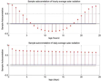
The autocorrelation functions computed for hourly and daily av-erage solar radiation time series are reported in Figure (2.4). As
Fig. 2.4. Autocorrelation of hourly and daily average solar radiation time series at Lambrate.
it is possible to see at hourly scale the autocorrelation function is strongly periodic with period 24 hours, as it was expected, due to the marked daily component which features solar radiation time series (see Figure (2.1) at hourly scale). Furthermore, the
autocor-16 2 Analysis of Solar Radiation Time Series
relation function computed at hourly scale decays at values lower than 0.37 (the so-called correlation time τc, in about 5 lags (hours), which is close to the δt ≃ 6, estimated from the time-space plot. At daily scale the autocorrelation reaches a minimum after a few (say 2 lags), but how it is possible to appreciate it decays very slowly.
However it is to bearing in mind that autocorrelation is a linear feature of time series. Since it is highly probable that solar radia-tion is generated by non linear processes, it is more appropriately to estimate also the mutual information, as shown in Figure (2.5). The Figure, in essence, confirms that at hourly scale the correlation
Fig. 2.5. Autocorrelation of hourly and daily average solar radiation time series at Lambrate.
2.4 Power Spectra 17
scale. This is a first assessment of the time horizon within which it is possible to make reliable predictions by using autoregressive models. However in this work, I have studied the prediction error in the overall range h ∈ [1, 24] for hourly average time series, as it will be described in Chap. 5.
2.4 Power Spectra
The power spectra of hourly and daily solar radiation time series are shown in Figure (2.6). It is possible to observe that at hourly scale
Fig. 2.6.Power spectrum densities of hourly and daily average solar radiation time series at Lambrate.
there are marked components with periods: T1 = 1/0.0001143 ≃ 8748 hours ≃ 1 year, T2 = 1/0.04167 ≃ 24 hours. The others
com-18 2 Analysis of Solar Radiation Time Series
ponents of the spectrum computed at hourly scale corresponding to periods of 12 hours, 6 hours etc, are well known effects of the considered Fast Fourier Transform (FFT) computing algorithm. At daily scale only one marked component is evident, corresponding to a period of T3 = 1/0.002743 ≃ 365 days, i.e. 1 year.
Further, Figure (2.6) shows that the slope of the power spectrum is about −1.33 at hourly scale and −0.54 at daily scale. The difference among these slopes can be easily explained bearing in mind that daily average solar radiation time series are less autocorrelated then the corresponding hourly average time series, and thus more similar to a white noise. Based on slopes of power spectra, it is possible to say that solar radiation time series belongs to the ubiquitous 1/f noise.
2.5 Hurst Exponent and Fractal dimension
The Hurst exponents and the fractal dimensions of hourly average time series computed for ten years at one of the considered record-ing stations are shown in Figure (2.7). The Hurst exponent was computed by using the R/S algorithm while the fractal dimension was computed by using the boxcounting algorithm. It is possible to see that, H and D, computed on windows of 1 year, gives on average H = 0.75 and D = 1.3. Thus the Hurst exponent is close to the range 0.73 ± 0.09 observed for several natural time series. Further-more it is possible observe that the theoretical relation H = 2 − D approximately holds.
2.6 Multifractal spectrum of solar radiation 19
Fig. 2.7. Hurst exponent and Fractal dimension of hourly average solar radiation time series at Lambrate.
2.6 Multifractal spectrum of solar radiation
Results of multifractal analysis performed on solar radiation time series is shown in Figure (2.8). In more detail, the left-upper sub Figure shows, in a log-log scale, the scaling function Fq versus the scale (from 64 to 4096 samples), for various values of the q (the local order of the local fluctuation exponent). Here it is to bear-ing in mind that negative q-order, e.g. (q = −5), amplifies the segments in the multifractal time series with extreme small fluctu-ations, whereas positive q-order e.g. (q = 5), amplifies the segments with extreme large fluctuations. The midpoint q = 0 is neutral to influence of segments with small and large fluctuation. Finally ob-serve that the slope of the regression lines, is the Hurst exponent
20 2 Analysis of Solar Radiation Time Series
Fig. 2.8. Multifractal spectrum at Lambrate (Milan) (hourly average from 2012 to 2014)
H corresponding to the considered q, also referred to as the gen-eralized Hurst exponent H(q). Here it is to be stressed that while a mono-fractal time series exhibits regression lines with the same slope for various q, this is not the case of solar radiation time series. Indeed, in the considered example (see the top rightmost sub Fig-ure (2.8)) the q-order Hurst exponent varies from 1.26 to 0.84 when q varies from -5 to 5. In more detail, it should be stressed that for q = 2 the generalized hurst exponent gives the Hurst exponent on the ordinary (i.e. mono fractal) fluctuation analysis. Such a value is usually a little different from the Hurst exponent obtained by using the R/S algorithm considered in section 2.5. The so-called mass exponent τq versus q, which is related to the q-order Hurst exponent, H(q), by expression (2.1)
2.6 Multifractal spectrum of solar radiation 21
τ (q) = qH(q) − 1 (2.1)
is shown in the leftmost bottom sub Figure (2.8). This curve, in case of a mono-fractal time series is exactly a straight line, since in this case the q-order Hurst exponent is independent on q. As it is possible to observe this is not the case of solar radiation, since in this case we have a curve with the concavity facing down. Finally the multi fractal spectrum (also referred to as singularity spectrum) is shown in the lower rightmost sub Figure (2.8). As in general the multi fractal spectrum assume an asymmetric bell shape with the maximum obtained for q = 0, in the example shown in Figure the spectrum is left truncated. This simply means that while large fluc-tuation scales within a limited range of Lipshitz-Holder exponents in the range (α ∈ [0.8, 0.9]), the small fluctuation scales following a winder range of exponents (α ∈ [0.9, 1.5]). This feature, seems to be shared by solar radiation time series recorded in different areas, as shown in Figure (2.9.b). In the Figure the singularity spectrum of solar radiation at five stations is shown. Four of the stations, re-ferred to as Lamb (Lambrate, Milano), Casa (Casatenovo, Lecco), Stez (Stezzano, Bergamo) and Como (Como), respectively are lo-cated in Lombardia while Aber is lolo-cated at Aberdeen (Ohio,USA). While the four recording stations located in Lombardia are all in the Po Valley at low altitude, Aberdeen is located in USA at 1433 m a.s.l. Probably the different altitude of the recording station may explain why singularity spectrum at Aberdeen is less wide, i.e. more close to be monofractal, with respect to the others.
22 2 Analysis of Solar Radiation Time Series
(a)
(b)
Fig. 2.9.Generalized Hurst exponent and singularity spectrum at four solar radiation recording stations (a) Generalized Hurst (b) Multifractal Spectrum.
2.7 Estimation of the embedding dimension 23
2.7 Estimation of the embedding dimension
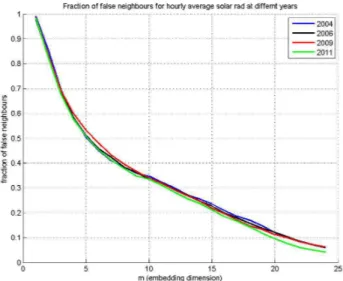
In order to determine the embedding dimension m of solar radiation time series, I have evaluated the fraction of false nearest neighbors versus m, as shown in Figure (2.10). The Figure shows that the
Fig. 2.10. Fraction of false nearest neighbors of solar radiation at Lambrate at different
years-fraction of false nearest neighbors decays very slowly with the em-bedding dimension, without reaching the zero value in the range m ∈ [1, 30]. This results could means that the supposed non-linear dynamical system, underlaying the solar radiation process in not low dimensional; however, it could also be interpreted as the effect of noise in the considered time series.
24 2 Analysis of Solar Radiation Time Series
2.8 Maximal Lyapunov exponent
Lyapunov exponents are an important means of quantification for unstable systems. They are however difficult to estimate from time series. Unless the underlying dynamical system is low dimensional and high quality data are available, it is non recommended to pute the full spectrum and at most it is recommended try to com-pute the maximal exponent only. To this purpose, I have consid-ered the lyapk function which is part of the TISEAN package. Re-sults obtained by using this algorithm on hourly average time series recorded at different stations indicate the existence of positive max-imal exponents in the range [0.6, 1].
2.9 Conclusions
Analysis presented in this chapter, performed on both hourly and daily average solar radiation time series allow to draw some conclu-sions about their nature. Stationary analysis, carried out by differ-ent approaches, has not pointed out evidences that they are nonsta-tionary, at least for time intervals of ten years, which is the largest considered in this study. The power spectrum analysis showed, in addition to the obvious presence of seasonal (mainly the daily and yearly) components, also that the slopes of the solar radiation time series power spectra are in the range [0.5, 1.5], which, according with claims existing in literature, means that solar radiation time series belong to the wide class of 1/f noise. Correlation analysis, carried out by using linear and non linear approaches, pointed out that solar radiation time series exhibits a correlation time of about
2.9 Conclusions 25
τc = 5 lags at hourly time scale and of about τc = 1 lag at daily scale, which means that prediction models, based on autocorrela-tion only, have limited chances to be reliable, unless that for very short horizons. Fractal analysis pointed out that these kind of time series are fractal exhibiting, on average, fractal dimension D = 1.3 and Hurst exponent of H = 0.75. Furthermore, the Multi-Fractal Detrended Fluctuation Analysis (MFDFA) has pointed out that solar radiation time series are multi-fractal, exhibiting singularity spectra, computed for different recording stations and geographic areas, that are usually left-truncated, which means that while large fluctuation scales within a limited range of Lipshitz-Holder expo-nents (α ∈ [0.8, 0.9]), the small fluctuation scales following a wider range of exponents (α ∈ [0.9, 1.5]). Analysis carried out in order to see if there are evidences of deterministic chaos give controversial results. Indeed, the search for an embedding dimension pointed out that there is still a limited (i.e. ≤ 0.1) fraction of false nearest neigh-bors at high, dimension (e.g. m = 24). This results can be explained in different ways: the high embedding dimension is the effect of un-avoidable noise in the time series or simply a low dimension chaotic attractor does not exists. On the other hand the computation of the maximal Lyapunov exponent has pointed out that there is at least a positive exponent in the range [0.6, 1], thus meaning that a chaotic attractor could be hypothesized. In conclusion, since as well-known the computation of Lyapunov exponents from time series is quite difficult, at the present stage of this research, it is possible to affirm that while there are enough evidences to say that solar radiation time series belong to the large class of multifractal 1/f noises, there
26 2 Analysis of Solar Radiation Time Series
are not enough evidences to assess that a low dimensional chaotic attractor underlies the considered solar radiation time series.
3
Analysis of Wind Speed Time Series
The purpose of this chapter is to analyze a representative data set of wind speed time series recorded both in Italy and USA. The considered recording stations in Italy are mainly lo-cated in Lombardia and were provided both by the Politec-nico di Milano (Como Campus) and by the ARPA Lombardia (see http://ita.arpalombardia.it/ita/index.asp). The sta-tions located in USA are a subset of the Western Wind Resource (WWR) Dataset, modeled in the framework of the Western Wind and Solar Integration Study (see http://wind.nrel.gov/). Origi-nal time series were available with different sampling time: 5 min for the Como Campus data set, 10 min, for the WWR data set and 1 hour for the ARPA Lombardia data set. Data of the Como Campus station was recorded from 2011 to 2013, while the WWR dataset was recorded from 2004 to 2006; finally, data of the ARPA Lombar-dia is in general available since 2004. As for solar raLombar-diation, analysis performed on wind speed time series was devoted to assess general features such as stationarity, power spectrum, autocorrelation and mutual information, fractal and multifractal features, as suggested
28 3 Analysis of Wind Speed Time Series
by [7]). Furthermore, some kind of analysis were performed in or-der to assess the hypothesis of low dimensional chaos in wind speed time series, as claimed by ([8]). Some of the ideas described in this section were proposed in [9].
Description in this Chapter starts showing (see Figure (3.1)) that wind speed, such as solar radiation, are fluctuating time series at any time scale. However, of course, this not automatically implies
Fig. 3.1.Wind speed time series recorded at station ID2257
that they are nonstationary, as shown in the next section.
3.1 Stationary analysis
Stationary analysis was performed by various techniques, including the Augmented Dicky-Fuller (ADF) test, the Phillips-Pearson (PP)
3.2 Autocorrelation and Mutual Information 29
test, and the variance ratio (VR) test. All test rejected the null hypothesis, thus meaning that there are not enough evidences to assess that the considered time series are nonstationary, at least for time scale of three years. I tried also to assess stationarity by considering the recurrence plots. Recurrent plots of hourly wind speed time series, for different embedding dimensions, are shown in Figure (3.2). The uniform distribution of dots in the recurrent plots indicates that there are not particular structures that could be related with non stationarity, thus confirming achievement of the ADF, PP and VR tests.
3.2 Autocorrelation and Mutual Information
The power spectrum and autocorrelation function computed on hourly average wind speed time series are reported in Figure (3.3). As it is possible to see at hourly scale the autocorrelation function exhibits a slow decaying behavior, which is typical of 1/f noise. Indeed autocorrelation at daily scale decays at meaningless lev-els in about 3 lags. Autocorrelation of wind speed time series was also estimated in terms of mutual information, as shown in Figure (3.4). The Figure, in essence, confirms that the correlation time τc is about 6 lags at hourly scale and 2 lags at daily scale. This is a first assessment of the time horizon within which it is possible to make reliable predictions by using autoregressive models. However, in this work, I have studied the prediction error in the overall range h ∈ [1, 24].
30 3 Analysis of Wind Speed Time Series
(a)
(b)
Fig. 3.2. Recurrence plots of hourly wind speed at station ID 2257 during 2004 for different embedding dimensions (a) m=1 (b) m=2
3.3 Power Spectra 31
Fig. 3.3. Autocorrelation of hourly and daily average solar radiation time series at the ID2257 station.
3.3 Power Spectra
Typical power spectra of hourly and daily average wind speed time series are shown in Figure (3.5). It is possible to observe that at hourly scale there are components with periods: T1 = 1/0.0001143 ≃ 8748 hours ≃ 1 year, T2 = 1/0.04167 ≃ 24 hours. At daily scale only a component is evident corresponding to a period of T3 = 1/0.002743 ≃ 365 days, i.e. 1 year. The absolute slopes of hourly and daily average wind speed power spectra computed for some of the considered stations are reported in Table 3.3. As it is possible to see for the stations referred as Aberdeen, Chiari, Como, Lambrate and Vercana the slopes both at hourly and daily scale are in the range β ∈ [0.51.5], thus meaning that performs as 1/f
32 3 Analysis of Wind Speed Time Series
Fig. 3.4. Mutual information of hourly and daily average wind speed time series at the ID2257 station.
station β(hourly) β(Daily) Aberdeen 1.50 0.80 ID2257 2.01 0.96 ID2300 2.03 0.92 ID6435 1.87 0.74 ID9004 1.84 0.78 Chiari 1.44 0.62 Como 1.26 0.67 Lambrate 1.34 0.71 Vercana 1.55 0.74
Table 3.1. Absolute slopes of hourly and daily average power spectra at various stations in USA and Italy
noise. Instead, for the stations referred to as ID2257, ID2300,ID6435 and ID9004, the time series exhibit absolute slopes almost close to
3.4 Hurst Exponent and Fractal dimension 33
Fig. 3.5.Power spectrum densities of hourly and daily average solar radiation time series at the station ID2257.
2, thus behaving as random walks. The peculiarity of these latter stations is that wind is recorded at 100 m above sea level.
3.4 Hurst Exponent and Fractal dimension
The Hurst exponents and the fractal dimensions of hourly average wind speed computed for each year during 2004 to 2006 is shown in Figure (3.6). The Hurst exponent was computed by using the R/S algorithm while the fractal dimension was computed by using the boxcounting algorithm. It is possible to see that on average the Hurst exponent is 0.74 while the fractal dimension is 1.38. Thus the Hurst exponent is almost in the range 0.73 ± 0.09, observed for several natural systems. The Hurst exponent computed at nine
34 3 Analysis of Wind Speed Time Series
Fig. 3.6.Hurst exponent and Fractal dimension of hourly average wind speed at the station ID2257.
different recording stations by using three different algorithms [10], namely the R/S, the DF A and GP H, are given in Figure (3.7). As it possible to see there are clear differences among different algorithms. However all algorithms confirms that, independently from the considered recording stations and algorithm, wind speed time series are fractal and long range correlated, since the Hurst exponent are in the range 0.5 < H ≤ 1.
3.5 Multifractal Spectrum
Results of multifractal detrended fluctuation analysis performed on hourly average wind speed time series are shown in Figure (3.8). Roughly speaking this Figure shows that wind speed time series,
3.5 Multifractal Spectrum 35
Fig. 3.7.Hurst exponent computed at nine recording stations by three different ap-proaches. The nine recording stations are: 1 = Aberdeen,2 = ID2257,3 = ID2300,4 = ID6435,5 = ID9004,6 = ID9004,7 = Chiari,8 = Como,9 = V ercana
similarly to solar radiation time series, are multifractal. A detailed interpretation of this Figure is similar to that given in section 2.6 for the multifractal spectrum of solar radiation time series.
The generalized Hurst exponent and the corresponding multi frac-tal spectrum at various wind speed recording stations in USA and in Italy are shown in Figure (3.9) and Figure (3.10), respectively. Figure (3.9a) and (3.10.a) show that the generalized Hurst ex-ponent H(q) significantly varies versus q, thus meaning the clear multifractal nature of wind speed time series at all the considered stations, independently on the geographical area and altitude. In particular, bearing in mind that H(2), i.e. the generalized Hurst exponent obtained for q = 2, represents the Hurst exponent given
36 3 Analysis of Wind Speed Time Series
Fig. 3.8.Multifractal spectrum at station ID2257
by the traditional monofractal DFA (Detrended Fluctuation Anal-ysis), it is possible to see that such particular values are in the range H ∈ [0.65, 0.75] and H ∈ [0.7, 0.75] for the USA and Italy stations, respectively. Such a difference can be explained looking at the altitude (from the ground, or from the sea) at which wind speed is sampled and at the different altitude above sea level of the recording stations. Indeed stations referred to as ID2257, ID2300, ID6435 and ID9400 samples wind speed at 100 m from the ground (or form the sea, in case of offshore plants), while the remaining stations samples wind speed at 10 m from the ground. Furthermore stations ID2257, ID2300 belongs to offshore plants while stations ID6435, ID9400 and Aberdeen are located at about 1700, 2100 and 1437 a.s.l., respectively.
3.5 Multifractal Spectrum 37
(a)
(b)
Fig. 3.9. Generalized Hurst exponent and multifractal spectrum at various record-ing wind speed recordrecord-ing stations in USA (a) Generalized Hurst (b) Multifractal Spectrum
38 3 Analysis of Wind Speed Time Series
(a)
(b)
Fig. 3.10. Generalized Hurst exponent and multifractal spectrum at various record-ing wind speed recordrecord-ing stations in Lombardia (Italy) (a) Generalized Hurst (b) Multifractal Spectrum
3.6 Estimation of the embedding dimension 39
for the recording stations in USA and in Italy, respectively. From these Figures it is evident that the features of the singularity spec-tra are significantly affected by the different operating conditions of wind speed recording stations. This aspect, which seems to me quite intriguing, is leaved for future developments of this research.
3.6 Estimation of the embedding dimension
In order to determine the embedding dimension m of wind speed time series, I have evaluated the fraction of false nearest neighbors versus m, as shown in Figure (3.11). The Figure shows that,
simi-Fig. 3.11.Fraction of false nearest neighbors of solar radiation at Lambrate during 2012
40 3 Analysis of Wind Speed Time Series
of false nearest neighbors decays slowly with the embedding dimen-sion and a small fraction is computed also for m = 24. This results may be due to noise effecting the data.
3.7 Maximal Lyapunov exponent
I have estimated the maximal Lyapunov exponent of hourly average wind speed by using the approach described in [11]. Computation performed with the Lyap spec program, which is part of the Tisean package gives a value of 0.121. It is interesting to observe that similar values was observed for all considered recording stations. Furthermore, not only the largest Lyapunov exponent are almost equal but the overall Lyapunov spectrum, as shown in Figure (3.12).
3.8 Conclusions
Analysis presented in this chapter, performed on both hourly and daily average wind speed time series allow to draw some conclu-sions about their nature. Stationary analysis, carried out by using different approaches, has not pointed out evidences that they are non stationary, at least in time interval of a few years, as analyzed in this work. Fractal analysis pointed out that these kind of time series are fractal and, in more detail, multi-fractal. Some kind of analysis carried out in order to see if there are evidences of low dimensional deterministic chaos in wind speed in time series, as claimed by ([8]), is not clear to me. Indeed, the search for an em-bedding dimension, performed in the range [1, 24], pointed out that
3.8 Conclusions 41
Fig. 3.12.Lyapunov spectrum of hourly average wind speed at 4 different recording stations
there is a fraction of false nearest neighbors also for high embed-ding values (e.g. m = 24), thus meaning that the supposed low dimensional chaotic attractor is not realistic. However, this results can also be explained as the effect of random noise which affect the dataset. On the other hand the computation of the maximal Lyapunov exponent and of the whole Lyapunov spectrum pointed out the presence of one or more positive exponents. However, the spectral analysis show that wind speed time series, belongs to the class of 1/f noise or in same case to random walks.
4
Time series models for wind speed and
solar radiation
Research efforts in the area of wind speed and solar radiation time series forecasting started in the eighties and has becoming contin-uously increasing and nowadays some hundred thousand of scien-tific papers are available. However, since standard protocols are not considered to assess the features of the proposed models, it is very difficult, or even impossible, to inter-compare different techniques from literature results.
Referring to the subject of wind speed time series forecasting several review papers have been published such as [12],[13],[14],[15],[16], and [17]. Nevertheless, most of the paper agree to indicate that sta-tistical models perform well when the forecasting horizon is only a few hours.
After the earliest attempt to predict wind speed time series by using Kalman models [18], a huge number of techniques have been con-sidered such as ARMA (Auto Regressive Moving Average) models [19],[20],[21], ARMA-GARCH (Generalized Autoregressive Condi-tional Heteroskedasticity) [22], ARIMA and ANN (Artificial Neu-ral Networks) [23],[24], Hybrid models ARMA and TDNN (Time
44 4 Time series models for wind speed and solar radiation
Delay Neural Networks) [25], ANN (Artificial Neural Networks) [26],[27],[28], Soft-Computing models [29], ANFIS (Adaptive Neural Fuzzy Systems) [30], Generalized mapping regressors [31], Marcov chains [32], Principal Component Phase Space Reconstruction [33], Multiple architecture system [34] and Spatial Correlation models [35]. However such a list of modeling techniques is not exhaustive. Referring to the modeling of solar radiation time series, techniques similar to those referenced above for wind speed have been pro-posed. For instance, ARMA-GARCH models have been considered by [36], ARMA and TDNN by [37] and [38], Recurrent Neural Net-works by [39], ANFIS and ANN by [40] and [41], Statistical time series models by [42], Decomposition models by [43], Fuzzy with Genetic Algorithms models by [44], Empirical mode decomposition by [45], Bayesian statistical models by [46], Machine learning by [47], Particle swarm optimization and evolutionary algorithm, us-ing recurrent neural networks by [48]. Also in this case this list is far to be exhaustive.
In my PhD work, after trials with several of the approaches pro-posed in literature, I have decided to focus on the use of the NAR (Non-linear Auto Regressive) and EPS (Embedding Phase Space) model structures, identified by using ANFIS (Adaptive Neuro-Fuzzy Inference Systems) and ANN (Artificial Neural Networks) approaches, as described in the following section.
4.1 NAR and EPS time series models
A time series can be considered as a sequence of measurements y(t) of an observable y performed at equal time intervals. The Takens
4.1 NAR and EPS time series models 45
theorem implies that for a wide class of deterministic systems, there exists a diffeomorphism (i.e. a one-to-one differential mapping) be-tween a finite window of the time series (y(t), y(t−1), ..., y(t−d+1) and the state of the dynamic system underlying the series. This im-plies that in theory there exist a MISO (Multi-Input Single-Output) mapping f : Rn→ R such that
y(t + 1) = f (y(t), y(t − 1), ..., y(t − d + 1)) (4.1) where d (dimension) is the number of considered past values. This formulation returns a state space description where, in the d di-mensional state space, the time series evolution is a trajectory and each point represents a temporal pattern of length d. Prediction models of the kind (4.1) are usually referred as NAR (Nonlinear Auto-Regressive) models. These kind of models generalize into the so-called NARX (acronym of Nonlinear Auto-Regressive with eX-ogenous, i.e. external, inputs) model represented by expression (4.2) y(t + 1) = f (y(t), ..., y(t − d + 1), u(t), ..., u(t − q + 1)) (4.2) in presence of a vector u(t) of explaining variables, i.e. variables that are in some way correlated with y(t). NAR and NARX have a linear counterpart into AR and ARX which however are not usually appropriate to describe natural phenomena. Mapping of the kind (4.1) or (4.2) can be used in two ways: one-step prediction and iterated prediction. In the first case, the d previous values of the se-ries are assumed to be available and the problem is equivalent to a function estimation. In the case of iterated prediction, the predicted output is feedback as an input to the following prediction. Hence,
46 4 Time series models for wind speed and solar radiation
the inputs consist of predicted values as opposed to actual obser-vations of the original time series. A prediction iterated for k times returns a k-step-ahead forecasting. The task of forecasting a time series over a long horizon is commonly tackled by iterating one-step-ahead predictors. Despite the popularity that this approach gained in the prediction community, its design is still affected by a number of important unresolved issues, the most important being the accumulation of prediction errors. In my experience, iterated forecasting does not work after a very few steps. Another prob-lem dealing with NAR (and NARX) models is that the regressors (y(t), y(t − 1), ..., y(t − d + 1) of the output variable are the most recent past variables, which very often are correlated each other, i.e. are not really independent variables. To avoid using consecu-tive regressors of y(t) it is possible to modify the regressor vector as (y(t), y(t − τ ), ..., y(t − (d − 1)τ )), i.e. the regressors are time-spaced by τ steps and thus expression ((4.1)) could be modified as in expression (4.3).
y(t + 1) = f (y(t), y(t − τ ), ..., y(t − (d − 1)τ )) (4.3) The τ parameter is usually chosen with the criterion of the first minimum of the mutual information, which assures that two con-secutive regressors of the f function are few correlated and thus almost independent. These ideas are inspired by the so-called Em-bedded Phase-Space (EPS) representation of dynamical systems which are largely considered in non-linear modeling of chaotic time series. Of course expression (4.3) reduces to the traditional NAR form (4.1) when τ = 1. In the framework of EPS models the param-eter τ is referred to as delay while d is referred to as the embedded
4.3 Mapping approximation 47
dimension and can be chosen by using various criteria such as, for instance, evaluating the fraction of false neighbors.
4.2 Multi-step ahead prediction models
The MISO map (4.3) can be appropriately extended for multi-step prediction according with expression (4.4).
y(t + h) =f (y(t), y(t − τ ), ..., y(t − (d − 1)τ )
h = 1, 2, ...24 (4.4)
In other terms, in order to perform multi-step prediction avoiding to use iteratively expression (4.2), which as mentioned fails after a few step due to accumulation error, it is proposed to directly map-ping the input vector [y(t), y(t − τ ), ..., y(t − (d − 1)τ ] to the output scalar y(t + h) by using two different neural network based ap-proach, namely the Neuro-Fuzzy (NF) and the Feedforward Neural Network (NN) approaches. The mapping will be performed for pre-diction horizon h in the range 1 ≤ h ≤ 24 hours. The two mapping approaches are shortly outlines in the next sections.
4.3 Mapping approximation
Neural Networks based approaches are among the most popular and efficient tools to approximating a map f of the kind consid-ered in this work. In particular, I have considconsid-ered two kinds of approaches namely the Neuro-Fuzzy and the Feedforward Neural Networks approaches, respectively. One of the main advantages of
48 4 Time series models for wind speed and solar radiation
these approaches is that, roughly speaking, they allow to approx-imate nonlinear maps by various kinds of basis function, such as, sigmoidal, gaussian, wavelet and so on. In particular the gaussian basis functions seems particularly appropriate for solar radiation time series modeling, due to the gaussian shape of daily solar time series.
4.3.1 The Neuro Fuzzy approach
One of the most interesting aspects of the NeuroFuzzy approach is that once the neural network has been trained by using auto-matic learning algorithms, the obtained model can be interpreted in terms of a base of if ... then rules. The resulting models can be represented both in linguistic form, or as multidimensional surfaces, whose coordinates are the arguments of the f function. In partic-ular, if the rules are expressed in the so-called Takagi-Sugeno form [49], i.e with the consequent part expressed as a linear combination of the input mapping, often the model surfaces are iperplanes and thus the rule base can be approximated by simple mathematical ex-pressions. Identification of the model rule base can be obtained in several ways. In particular I have considered the genfis3.m function which is part of the Maltab fuzzy toolbox. This function generates a FIS (Fuzzy Inference System) by using the fuzzy c-means (FCM) clustering algorithm. Gaussian type functions were considered to represent the membership functions. For each of the argument that appears in the f function, three membership functions were consid-ered to describe what is usually referred the universe of discourse. In this work, the combination of the Embedded Phase Space model
4.4 Conclusions 49
structure and the Neuro-Fuzzy neural networks for approximating the f map, will be referred, to as the EPSNF approach.
4.3.2 The FeedForward Neural Network Approach
Feedforward networks consist of a number of simple artificial neu-rons, organized in layers. The first layer has a connection from the network input. Each subsequent layer has a connection from the previous layer. The final layer produces the network’s output. Such a kind of networks can be used for many kinds of input to output mapping. A feedforward network with at least one hidden layer and enough neurons can fit any finite input-output mapping problems. Several kind of different training algorithm can be used to training the network, such as for instance the popular Levenberg-Marquardt optimization algorithm which was taken into account in this work. Since in this case feedforward neural networks are considered for approximating the f map, the approach will be referred to as EP-SNN.
4.4 Conclusions
A huge number of techniques have been proposed in literature to model solar radiation and wind speed time series and thus it is al-most impossible to be exhaustive dealing with this subject. For this reason, the description was limited to the NARX and to the Em-bedded Phase-Space approaches, which were considered the most appropriate for the purposes of this work.
5
Modeling hourly average solar radiation
time series
In this section results obtained by applying the modeling ap-proaches described in Chap. 4 to a data set of hourly average time series recorded from 2011 to 2013 are reported. For all modeling tri-als, data recorded during 2011 and 2012 was considered to identify the model parameters while remaining data was reserved to test the model. Model performances have been evaluated by considering the traditional mae and rmse error indices.
5.1 Performances of the NARX Neuro-Fuzzy
modeling approach
One of the interesting aspects of applying the Neuro-Fuzzy tech-nique to the considered problem is that it is often possible to obtain quite simple approximated models which relate the solar radiation at some time (t + h) and others meteorological variables recorded at the same station until time t. The description starts showing results obtained by the simple model of the form (5.1), where the prediction horizon has been set to h = 0, which means a pure
52 5 Modeling hourly average solar radiation time series
static input-output model, with the aim of evaluating to what ex-tent the hourly average solar radiation at time t can be explained as a function of the hourly average values of temperature, pressure and relative humidity recorded at the same hour.
sr(t) = f (ws(t), te(t), pr(t), hum(t)) (5.1) The Neuro-Fuzzy model obtained, graphically represented in terms of surfaces in three dimensional spaces, consists of planes, as shown in Figure (5.1) and thus a simple mathematical representation of the model is possible, as expressed by equation (5.2).
sr(t) =13.8 · ws(t) + 7.3 · te(t) + 1.74 · pr(t)
− 2.5 · hum(t) − 1615 (5.2)
The time behavior of such a model, represented in Figure (5.2), shows that it perform poorly, i.e. it is only partially able to capture the true relation among solar radiation and the other considered explaining variables. On the other hand the hourly averages of solar radiation are weekly correlated with the explaining variables considered in equation (5.2). For short time horizons, such a be-havior can be significantly improved, by adding and autoregressive term, i.e. considering, in the simplest case, a model of the form (5.3).
sr(t + h) =f (sr(t), ws(t), te(t), pr(t), hum(t)),
h = 1, 2, ... (5.3)
as shown in Figure (5.3) for h = 1. It is evident that adding at least one regression of the output into the list of the f arguments improves the capability of the model to predict future values
(com-5.1 Performances of the NARX Neuro-Fuzzy modeling approach 53
54 5 Modeling hourly average solar radiation time series
Fig. 5.2.True and modeled time series by a NARX NF model expressed by equation 5.1 (h=0).
pare the behavior shown in Figure (5.2) with that shown in Fig-ure(5.3). In order to objectively evaluate the performance of NF models of the form (5.3) for the whole range 1 ≤ h ≤ 24 of pre-diction horizon, two error indices were computed: the mae (mean absolute error) and the rmse (root square mean error), defined as expressed in (5.4) and (5.5), respectively.
mae = 1 n n X i=1 |y(i) − ˆy(i)| (5.4) rmse = v u u t 1 n n X i=1 (y(i) − ˆy(i))2 (5.5)
where n is the number of samples considered to compute the er-ror indices and the symbol ˆy indicates the estimated sample.
Fur-5.1 Performances of the NARX Neuro-Fuzzy modeling approach 55
Fig. 5.3.True and modeled time series by a NARX NF model expressed by equation (5.3) (h=1).
thermore the NF model performance was compared with that of a persistent model, i.e. a model characterized by the simple equation (5.6), which is often considered as a reference model.
ˆ
y(t + h) = y(t) (5.6)
From results shown in Figure (5.4) it is possible to see that: 1. for 1 ≤ h ≤ 4, the model (5.3) performs exactly as the persistent
model and thus there is not convenience on using it.
2. The mae and rmse, increases faster for the persistent model with respect to the NF model. Furthermore, while for the NF model the error reaches a maximum value for h = 5, for the persistent model the error curve is almost symmetric and reaches a max-imum for h = 12, i.e. half of a day. For h > 12 the persistent
56 5 Modeling hourly average solar radiation time series
model error start decreasing and for h = 24 again approaches values comparable to that of the NF model.
3. for 21 ≤ h ≤ 24 again the NF model performs as the persistent. 4. Although the NF model outperform the persistent model for prediction horizon in the range 5 ≤ h ≤ 20, this does not imply that its performance are acceptable for forecasting purpose, even at short time horizon. For instance, its time behavior for h = 3 is shown in Figure (5.5), which reveals that the model is not reliable to predict the peak values of the true time series.
5.2 Performances of the NARNF approach
In this section models of the form 4.1, for different values of the delay d in the range [3, 24] are considered. The mae and rmse errors obtained for this kind of models are shown in Figure (5.6). It is possible to see that NARNF models featured by τ = 1 do not exhibits a uniform error versus h in the overall explored range, unless the dimension d is set to d = 24. Instead, the NARNF model with an embedding dimension d = 24 perform quite well, not only for short prediction horizons but in the whole range [1, 24] since the mae and rmse curves are flat. In terms of performance indices, it is possible to say that mae ≤ 50W/m2
and rmse ≤ 90W/m2
in the whole explored range.
5.2 Performances of the NARNF approach 57
58 5 Modeling hourly average solar radiation time series
Fig. 5.5.True and modeled time series by a NARX NF model (h=3).
5.3 Performances of the EPS Neuro-Fuzzy
modeling approach
In this section I show results obtained considering embedding phase-space models of the form (5.7),
sr(t + h) =f (sr(t), sr(t − τ ), ..., sr(t − (d − 1)τ )
h = 1, 2, ...24 (5.7)
where, again, the unknown mapping function f is identified by the neuro fuzzy approach. In the rest of the work this kind of models will be referred to as EPSNF (acronym of Embedded Phase-Space Neuro-Fuzzy). Since the most appropriate value for the embedding dimensions is unknown, a series of trials were performed assuming that d is an integer value in the range 3 ≤ d ≤ 24. As concerning the
5.3 Performances of the EPS Neuro-Fuzzy modeling approach 59
60 5 Modeling hourly average solar radiation time series
delay τ , two series of trials were performed. The first trial assumes τ = 1, since this is the case when the EPS model reduces to the popular NAR model. The second series of trial refers to different values τ > 1.
5.4 Performances of the EPSNF approach
In this section prediction models of the form (4.3) identified by us-ing the NF mappus-ing approach are considered by settus-ing the time delay parameter τ = 2 and for various values of d in the range [3, 24]. The performance in terms of mae and rmse are shown in Figure (5.7). It is possible to see that NAR NF models do not ex-hibits a uniform error versus h in the overall explored range, unless the dimension d is set to d = 12. Thus it was experimentally found that an EPS model with 12 regressors perform as a NAR model with 24 regressors, provided that the 12 regressors are chosen as-suming τ = 2. This results can be explained bearing in mind that hourly average solar radiation time series exhibits a strongly peri-odic behavior with a 24 hours period and that by using 12 regressors delayed by τ = 2 it is possible to cover the whole 24 hours time interval. Furthermore, it is to stress here that the search for an em-bedding dimension for hourly average solar radiation time series, by using the false-neighbors algorithm suggested an embedding di-mension ≥ 24. This result allows to conjecture that to implement a prediction model with flat mae and rmse errors in the whole range [1, 24], it is required, that d · τ ≥ 24. Such a conjecture was experi-mentally verified to be true as shown in Figure (5.8). It is possible to observe that the error curves, obtained assuming d·τ = 8·3 = 24
5.4 Performances of the EPSNF approach 61
62 5 Modeling hourly average solar radiation time series
Fig. 5.8.mae versus the horizon for an EPSNF model (d · τ = 24).
works as well as the model featured by d · τ = 12 · 2 = 24. However the figure shows that there is a minimum value for the number of regressors. Indeed, for instance choosing d = 8 and τ = 3 or d = 6 and τ = 4 do not give flat error over the explored range. Thus the rules should be modified as follow: to obtain an almost flat error it is necessary that both these to relations hold: d · τ ≥ 24 and τ ≤ 3. To further stress the convenience of using the NF approach in con-junction with the EPS model structure it is reported in equation (5.8), the mathematical representation of an EPSNF model having (d = 8, τ = 3) and h = 5.
5.5 Performances of the NARNN approach 63
sr(t + 5) =0.0510sr(t) + 0.7866sr(t − 3) + 0.0796sr(t − 6)+
− 0.0383sr(t − 9) − 0.0144sr(t − 12) − 0.0041sr(t − 15)+ − 0.0342sr(t − 18) − 0.0008sr(t − 21) + 16.1475
(5.8) which is quite simple to implement.
5.5 Performances of the NARNN approach
In this section performance of EPSNN, here considered as the acronym of Embedded Phase-Space Neural Network models will be shortly reported. For the lack of brevity, it is possible to say that considerations already expressed in the previous section for models EPSNF can also be applied to models EPSNN. For instance, the performance of the EPSNN model (5.7), in terms of mae and rmse errors are synthesized in Figure (5.9) for various embedding dimen-sion d and also in comparison with the persistent model. The Figure shows that the EPSNN models significantly outperform the persis-tent model for any value for the embedding in the range considered (3 ≤ d ≤ 24). It is worth nothing that the performance for d = 12 and d = 24 are almost identical, thus demonstrating experimentally that, as already shown for models EPSNF d = 12 is probably the most appropriate size of the embedding for the considered problem, when using the NAR model structure. Another interesting aspect is that performance of this kind of models are almost independent on the prediction horizon in the range 1 ≤ h ≤ 24.
64 5 Modeling hourly average solar radiation time series
Fig. 5.9.Performances of the EPSNN models for τ = 1 and d ∈ [3, 8, 12, 24](a) mae (b)rmse.
5.6 A direct comparison between the EPSNF and EPSNN approaches 65
5.6 A direct comparison between the EPSNF
and EPSNN approaches
A direct comparison between EPSNF and EPSNN models, working on the same data set, limited to embedding dimension of d = 12 and d = 24, is reported in Figure (5.10). The Figure shows that the EPSNN model with d = 12 is slightly more accurate than cor-responding EPSNF model and therefore may be preferred, in this respect. However this small advantage may not be decisive since the EPSNF models allow a simple external representation with re-spect to EPSNN model. Further insights concerning the goodness of EPSNN models can be obtained from the analysis of the resid-ual, i.e. the difference between the actual and the predicted time series. To this purpose, as an example, the autocorrelation of the true and residual time series corresponding the prediction with a time horizon of h = 5 is shown in Figure (5.11). It is possible to see that both the autocorrelation and the mutual information of the residual decay faster than that of the true time series and periodic behavior is strongly attenuated in the residual time series. The his-togram of residual generated by the considered EPSNN model is shown in Figure (5.12). The Figure shows that the residue of so-lar radiation generated by the model considered is symmetrically distributed around zero. In more detail, the central bin is centered at the value −24.04 and almost 80% of residual samples are in the central bin, while the remaining 20% is distributed around two bins: one with the center around the −136.11 value and the other centered at 88.02 -value.
66 5 Modeling hourly average solar radiation time series
Fig. 5.10. Performances of EPSNF and EPSNN models for different embedding dimension (a) mae (b)rmse.
5.6 A direct comparison between the EPSNF and EPSNN approaches 67
Fig. 5.11. Autocorrealtion and mutual information of the true and residual time series (h=5).
68 5 Modeling hourly average solar radiation time series
5.7 Conclusions
Results discussed in this chapter can be summarized as follows. Accuracy estimation of the prediction models, assessed in terms of mae and rmse gives mae ≤ 50W att/m2
and rmse ≤ 80W att/m2 , for the whole explored prediction horizon h ∈ [1, 24]. For very short prediction horizon, (h ≤ 3), the performances are better since it has been found mae ≤ 40W att/m2
and rmse ≤ 60W att/m2 . The studied models significantly outperform the persistent model in the whole explored prediction horizon h ∈ [1, 24]. The residue of solar radiation generated by the studied models is symmetrically dis-tributed around zero and almost 80% of residual samples are in the central bin. The NF and NN approaches considered to identify the non-linear map underlying NARX and/or EPS models are compa-rable in terms of accuracy. However, NF prediction models could be preferred since allow a relative simple external representation.
6
Modeling hourly average wind speed
time series
In this section results obtained by applying the modeling ap-proaches described in Chap. 4 to the data set of hourly average time series recorded at Como (Italy) from 2011 to 2013, are dis-cussed as a case of study. For all modeling trials, data recorded during 2011 and 2012 was considered to identify the model param-eters while data recorded on 2013 was reserved to test the model. Model performances have been evaluated by considering the tra-ditional mae and rmse error indices expressed by (5.4) and (5.5), respectively.
6.1 Performances of the NARNF approach
Following the same scheme adopted in the previous chapter devoted to solar radiation, I start the description of results obtained for wind speed time series from the simplest kind of NARX models, with the aim of evaluating to what extent solar radiation, temperature, air pressure and relative humidity may contribute to explain the wind speed dynamic at the considered recording site. Thus I have test