Isospin influence on dynamical and statistical emission of heavy fragments in heavy ion collisions at Fermi energies

Dottorato di Ricerca in Fisica - XXIX Ciclo

Isospin influence on dynamical and

statistical emission of heavy

fragments in heavy ion collisions at

Fermi energies

Sebastianella Norella

PhD Thesis

Coordinatore:

Prof. L. Torrisi

SSD: FIS/04

Tutor:

Prof. A. Trifir´

o

Co-Tutor:

Dott. P. Russotto

Introduction 3 1 Heavy Ion Collisions at intermediate energies 5

1.1 Semi-peripheral reactions at Fermi energies . . . 5

1.2 Dynamical and statistical effects in heavy ion collisions . . . 10

1.2.1 Dynamical fission as seen in the REVERSE experiment. . . 14

1.3 Theoretical models . . . 24

1.3.1 CoMD-II model . . . 24

1.3.2 BNV stochastic transport model . . . 29

1.4 InKiIsSy experiment: open question . . . 33

2 Experimental setup 34 2.1 CHIMERA multidetector . . . 34

2.1.1 The telecopes of CHIMERA array . . . 36

2.2 Electronic chain . . . 39

2.2.1 The electronic chain of silicon detectors . . . 40

2.2.2 The electronic chain of CsI(Tl) crystals . . . 42

2.3 FARCOS array . . . 43

2.3.1 Basic characteristics of FARCOS array . . . 45

2.4 Identification techniques . . . 46

2.4.1 ∆E-E technique . . . 47

2.4.2 The Pulse Shape Discrimination (PSD) in CsI(Tl) scintillators . . . 49

2.4.3 Time Of Flight (TOF) technique . . . 51

2.4.4 The Pulse Shape Discrimination (PSD) in Si detectors . . . 55

3 Telescopes response classification 60 3.1 Classification method . . . 60

4 Analysis and experimental results 68 4.1 Global variables . . . 68

4.2 Dynamical fission . . . 72

4.3 Velocity distribution . . . 80

4.4 Angular distributions . . . 82

4.5 Relative velocities . . . 85

4.6 Dynamical and statistical IMF production . . . 87

4.7 N/Z isotopic distributions . . . 90

Conclusion 94

A Cavata method to estimate impact parameter 96

In semi-peripheral heavy-ion collisions at Fermi energies (20-100 AM eV ), the reac-tion dynamics result mainly in binary products such as excited projectile-like (PLF) and target-like (TLF) fragments, that de-excite following an evaporation path. However also a dynamical IMFs (Intermediate Mass Fragments, defined as fragments of atomic number Z ≥ 3) emission can take place. The production of these IMFs is due to different reaction mechanisms and different time scales [1]. The analysis of previous experiments (REVERSE and TIMESCALE), in which the systems124,112_Sn+64,58_{N i at 35 AM eV beam energy have}

been studied, has shown a well-defined chronology: light fragments (Z < 9) are mainly emitted in fast fragmentation of neck connecting PLF and TLF, while the emission of IMF with Z ≥ 9 occurs at a later stage of the neck expansion process and it is dominated by an asymmetric mass splitting of the PLF in an aligned break-up configuration (“dynamical fission”) or by a sequential statistical decay of the PLF. These different decay patterns for the PLF break-up are characterized by peculiar angular distributions. In order to estimate the weight of these two components (dynamical and statistical) the fission-like angular distributions were used. It resulted that the dynamical component becomes more important with increasing energy dissipation and-or mass asymmetry. Comparing the two systems (124_{Sn +}64_{N i and} 112_{Sn +}58_{N i), it has been shown [2, 3] that while statistical}

fission probability is almost the same for the two reactions, the dynamical component is larger for the neutron rich system. This effect could be due to the different N/Z ratio of the two systems. However, some simulations have shown that it could also be related to the different size [4, 5].

In order to disentangle the effects related to the isopin from the ones related to the size of the two interacting systems, a new experiment, named InKiIsSy, has been carried out at Laboratori Nazionali del Sud in April 2013. During this experiment the 124_{Xe +}64_Zn

reaction has been studied at 35 AM eV beam energy, it has the same mass of the neutron rich system (124_{Sn +}64_{N i) and a N/Z ratio close to the value of the neutron poor one}

(112Sn +58N i). During the InKiIsSy experiment also the 124Xe +64N i system was ana-lyzed, in order to compare two systems (124Xe +64Zn and 124Xe +64N i) with same mass and beam but with different N/Z ratio for the target.

In this work the experimental results of these measurements will be shown, comparing them also with the ones of the REVERSE experiment.

Heavy Ion Collisions at intermediate

energies

1.1

Semi-peripheral reactions at Fermi energies

Semi-peripheral Heavy-Ion (HI) collisions at low energies (E < 10 AM eV ) are acterized by deep inelastic processes. The final states of these reactions are usually char-acterized by the presence of a massive fragment with velocity close to the projectile one, indicated with the term PLF (Projectile-Like Fragments), observed in coincidence with a fragment whose mass is close to the target one, indicated with the term TLF (Target-Like Fragment), as schematically shown in fig. 1.1. These primary fragments are often accom-pained by some reaction products coming from their statistical decay [6].

Increasing the beam energy into the Fermi energy domain (20-100 AM eV ), these binary

Figure 1.1: Schematic representation of semi-peripheral Heavy-Ion reaction at low energy (E < 10AM eV ).

reactions begin to be accompained by a copious emission of IMFs (Intermediate Mass Frag-ments), defined as fragments of atomic number 3 ≤ Z ≤ 20. IMFs show a typical kinemat-ics distribution centred at a velocity intermediate between that of Target-Like Fragment

and the one of Projectile-Like Fragment (fig. 1.2); it follows that their emission could not be explained by the statistical PLF or TLF decay alone [1, 7, 8, 9, 10, 11, 12, 13, 14]. The

Figure 1.2: Longitudinal velocity distribution of PLF, TLF and IMF for ZIM F s= 4, 8, 12, 18 for 124_{Sn +}64_{N i system [1].}

Figure 1.3: A schematic representation of neck emission process.

production of these IMFs may involve different timescales and different reaction mecha-nisms [1], ranging from a prompt fragmentation of the neck to a fast non-equilibrated fission-like mechanism or an equilibrated sequential decay. The observation of fig. 1.2 sug-gests that lighter IMFs are probably emitted from a transient neck matter zone connecting PLF and TLF, during reseparation of these two fragments. Fig. 1.3 shows a schematic representation of this neck emission process. Moreover light particles and IMFs emitted in the mid-rapidity region velocity are neutron richer than fragments statistically emit-ted from the PLF/TLF source [10]. Several experiments have been performed in order

to investigate the mechanisms of formation of these fragments. In particular, the sys-tems 124_{Sn +}64_{N i and} 112_{Sn +}58_{N i at 35 AM eV beam energy were investigated in the}

REVERSE experiment, performed at LNS of Catania. In ref. [1] the so-called “ternary events” were considered. They are those semiperipheral reactions in which one can observe a production of IMF in almost ideal condition, since the final-state configuration involves one IMF accompanying PLF and TLF. The REVERSE experiment was undertaken us-ing the forward part of CHIMERA array [15]. The inverse kinematics of these reactions allowed to detect and easily distinguish ternary events. Infact, in these conditions, the reaction products are focused at forward angle, where CHIMERA detector presents almost 85% of detection efficiency [16]. Fig. 1.4 presents the two-dimensional distribution of frag-ments for the124_{Sn +}64_{N i reaction as a function of Z of a given fragment and its parallel}

velocity along the beam axis. In this plot it’s possible to distinguish three strongly

popu-Figure 1.4: Distribution of fragments for the124Sn +64N i reaction as a function of their atomic number Z and their longitudinal velocity [1].

lated regions, recognized as PLF, TLF and IMF regions. In particular, the PLFs cover the area corresponding to heavy and relatively fast fragments of atomic number approaching the Z of Sn projectile (Zproj = 50) and moving with velocities close to the projectiles ones,

while TLFs cover the region around Z ∼ 18 and vlong ∼ 1 cm/ns. Instead, IMFs cover

the region of intermediate velocities. They are mostly light fragments, but they can have also larger Z values, up to Z = 18 − 20. As shown in fig. 1.2 where a plot of longitudinal velocity in laboratory reference frame for the three classes of fragments (PLF, TLF and IMF) for different ZIM F (IMF atomic number) in the case of 124Sn +64 N i reaction is

intermediate between the parallel velocities of TLF and PLF. Moreover, the longitudinal velocity of lighter IMF increases with increasing of IMF atomic number ZIM F, showing

a strong kinematical correlation with PLF for heavier IMF. In order to obtain important information on the mechanism of these ternary reactons, relative velocities characterizing binary subsystems of the total three body system were examined. In particular, correla-tions between relative velocities of IMF with respect to PLF (Vrel(IMF,PLF)) and TLF

(Vrel(IMF,TLF)) were analyzed. These relative velocities were normalized to the velocity

VV iola corresponding to the kinetic energy due to Coulomb repulsion for the binary

subsys-tems as given by the Viola systematic [17]. The correlation between relative velocities for ZIM F = 4, 8, 12, 18 are shown in fig. 1.5, from ref. [1]. This kind of correlation gives

infor-Figure 1.5: Correlations between relative velocities Vrel/VV iola(IMF,PLF) and

Vrel/VV iola(IMF,TLF) for different intermediate mass fragments of ZIM F = 4, 8, 12, 18.

Experimental distributions are compared with model calculations assuming that the IMF is released from the projectile (squares) or from target nucleus (circles) after a time interval of 40, 80 or 120 f m/c from the re-separation of the primary binary system at t = 0 [1].

PLF or TLF (or from both in the case of the instantaneous ternary split). The experimen-tal distributions are compared with model calculations assuming that the IMF is released from the projectile (squares) or from target nucleus (circles) after a time interval of 40, 80 or 120 f m/c from the re-separation of the primary binary system at t = 0 [1, 10]. Be-yond 120 f m/c the predicted points of the Vrel/VV iola(IMF,PLF) vs Vrel/VV iola(IMF,TLF)

correlation become undistinguishable from much later “true” sequential decay processes [18]. Specifically, considering the Vrel/VV iola(IMF,PLF) vs Vrel/VV iola(IMF,TLF) plots,

events close to the diagonal correspond to prompt ternary divisions (emission of IMF from the neck matter connecting PLF and TLF at its early stage of expansion), while events approaching Vrel/VV iola(IMF,PLF)=1 and Vrel/VV iola(IMF,TLF)=1 correspond to the

se-quential split of the primary projectile-like nucleus or the target-like nucleus, respectively. As it’s possible to see from the localization of events in the relative velocity correlation plot, the majority of light IMFs with ZIM F <∼ 10 are emitted in almost prompt or

“fast two-step” processes, within times of about 40-80 f m/c. Instead, the heavier IMFs (ZIM F >∼ 10) are preferentially emitted not immediately after reseparation of the

col-liding nuclei, but rather in somewhat later stage, starting at times of about 120 f m/c. Within the time interval of about 100 f m/c the studied system moves over a distance of about 20 f m, comparable with its size; so the emission of these IMFs (at times of about 120 f m/c) can still be associated with fragmentation of the neck formed between the nuclei after collision. This process is intermediate between a genuine prompt ternary decay of the colliding system and true sequential decay of projectile nucleus. In this case, in which the deduced time intervals extend up to 120 f m/c, it is possible that a two-step process takes place: the double break of a massive neck stretched between the receding nuclei, in which the neck first separates from TLF, and then breaks away from PLF. In this scenario, one can suppose that to form heavy IMFs more matter is required in the neck region, that is, the neck must be considerably stretched, so the second break of the neck must happen after a longer time. Sometimes, instead, the breaking of the neck can take place at its waist leaving most of the neck matter on one of the participating nuclei. This deformation could be absorbed with consequent statistical cooling, or, in others cases its relaxation could happen via a fragments emission. In this latter case heavy IMFs could be emitted by the fast splitting of a higly excited and deformed nucleus, a process that can be associated with the scenario of “Dynamical fission” reactions [19, 10]. In fact, the term “Dynamical Fission” indicates the process in which the projectile-like fragment (or target-like fragment), after interaction with the target (or the projectile), fissions so fast that angular distribution of fission fragments is not forward/backward symmetric. In both processes, dynamical fission and neck fission, a clear enhanced emission localized in the mid-rapidity region, intermediate between PLF and TLF rapidity, is obtained, resulting in

a clear anisotropy of the IMFs angular distributions, that indicates a preferential emission direction and an alignment tendency.

1.2

Dynamical and statistical effects in heavy ion

col-lisions

As previously said, in HI collisions the production of light charged particles and In-termediate Mass Fragments (IMFs) is due to different reaction mechanisms and involve different time scales, ranging from fast dynamical processes to statistical emission from equilibrated sources. The statistical aspects are dominant in low energy ractions (E <∼10 AM eV ) and, in this case, any memory of the entrance channel is forgotten. Instead, in Fermi energies regime dynamical aspects become more important. In particular, as dis-cussed in the previous paragraph, heavier fragments emission may be associated with a PLF binary-like splitting taking places ideally in dynamical or equilibrated way. These two different decay modes for the PLF break-up, are characterized by peculiar angular dis-tributions: an aligned break-up with the recoil velocity of the PLF source in the dynamical emission and an isotropic (neglecting spin effects) emission of fission-like fragments (in the PLF reference frame) in the sequential statistical decay.

In fact, in the case of sequential break-up both the dynamics of the previous collision and the characteristic equilibration times of various degrees of freedom come into play and the break-up step could give informations about dynamic and temporal aspects of the reac-tion. Varios experiments [20, 21] have shown that fission of hot nuclei occurs more slowly than as predicted by the standard transition-state theory of Bohr and Wheeler [22]. On the other hand, others obsevations point to opposite effect: a spectacular acceleration of nuclear fission. In order to investigate these effects, peripheral heavy ion collisions with three-four massive fragments in the exit channel were studied. In this respect, the sys-tems86_{Kr +}166_{Er and} 129_{Xe +}122_{Sn were investigated at 12.5 AM eV beam energy [23].}

For these reaction it was found that the three body events occur with a large probability with respect to the statistical model predictions. These events are mainly originated by a two-step mechanism and they are compatible with hypothesis of a binary deep-inelastic interaction, followed by the further fission-like decay of one of the primary fragments. Moreover, the magnitude of the modulation of energy released in the second fission step, induced by strong Coulomb proximity effects, depends on the time between first and sec-ond scission step. It establishes a clock of the order of 10−21 s, that is two order of magnitude smaller than time scale given by statistical framework. Besides, the angular distribution of the fragments was found consistend with an orientation of the fission axis approximately collinear with the axis of the first scission. All these features are consistent

with an intermediate fissioning system not fully equilibrated.

Further non-equilibrium effects were observed for the 100_{M o +}100_{M o and} 120_{Sn +}120 _Sn

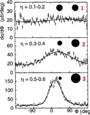
reactions, studied at 20 AM eV beam energy [9, 24]. Also here it was shown that, for the three-four heavy (with A ≥ 20) fragments events, the reaction takes place through a two-step mechanism: a first dissipative binary reaction between projectile and target, followed by a sequential fission decay. Considering the in-plane angular distributions (see next section for definition) for products of sequential fission of primary binary fragments (PLF or TLF) for various mass asymmetries (η = AHeavy−ALight

AHeavy+ALight) of the fission step (fig. 1.6), it’s

possible to see that, for moderate fission fragments mass asymmetry (panel 1), the angular distribution is quite flat. This indicates that there is not a preferential emission direction

Figure 1.6: In-plane angular distributions of sequential fission of primary binary fragments (PLF or TLF) produced in100M o+100M o reaction for various mass asymmetries, panel 1: η = 0.1−0.2, panel 2: η = 0.3 − 0.4, panel 3: η = 0.5 − 0.6, of the fission step [9, 24].

and the memory of the formation of the system is lost (pure sequential fission). Instead, increasing mass asymmetry, the angular distributions are peaked at small positive angles, which corresponds to an aligned configuration of the three nuclei: the non-fissioning pri-mary TLF (or PLF) and the two PLF (or TLF) fission fragments. Moreover, in this case, the smaller of the two fission fragments stays in the middle, demonstrating the persistency of a memory of the preceding deep-inelastic step and of direction of the separation axis between TLF and PLF. The observed forward/backward asymmetry indicates a short time

for the fission, that was there extrapolated following the model below exposed [9, 24]. In the case of asymmetric fission, fitting the angular distribution, the peak at small angles may be associated with an angle ϕm that describes the average rotation of the nucleus

from scission to scission. If the fissioning nucleus is characterized by a collective “angular velocity” ω, it’s possible to estimate the scission to scission lifetime as τ = ϕm/ω. In

particular, as shown in fig. 1.7, while at symmetry the scission to scission lifetimes are compatible with those expected for fission after attainment of global equilibrium, at high asymmetry lifetimes become of the order of 1 − 5 · 10−21s (typical of quasi-fission process), at least two order of magnitude smaller with respect to lifetime characteristic of a statisti-cal process [23]. In this case the second scission should happen after only a fraction of full

Figure 1.7: Scission to scission lifetime τ , extracted from angular distribution of figure 1.6, as a function of fission fragments mass asymmetry for 100M o +100M o and 120Sn +120Sn reactions around 20 AM eV . Moreover, statistical fission compatible lifetimes obtained in other studies [25] are reported.

rotation [26], without passing through the stage of a true compound nucleus. Therefore, HI collisions show PLF break-up, not only from statistical fission process, but also from a fast/non equilibrated break-up (dynamical fission).

Other studies on the binary break-up of PLF were made for various reactions (like Pb+Ag and Xe+Sn) and incident energies (20-50 AM eV ) [13]. For these systems it was found that, while for heavy projectiles impinging on light target (Pb+Al, U+C) the PLF break-up occurs mainly in two approximately equal size fragments (as expected for the statistical fission of a heavy nucleus), in the case of heavy targets (Pb+Au, U+U) the break-up of PLFs shows in addition an important contribution for the highest asymmetries, that in-creases with the size of the target. So, in this case, the break-up of PLF depends strongly

on the target size. Moreover, while for light targets the angular distributions of fission fragments are forward/backward symmetric in PLF reference system (as expected in stan-dard fission of a rotating nucleus), for heavy targets and greater fission fragments mass asymmetries the break-up axis is preferentially aligned with the separation direction of the two primary fragments (PLF and TLF), with the lighter fragments backward emitted in the PLF reference (aligned break-up). In ref. [13] the relative importance of these mechanisms has also been quantified. In the case of Pb+Ag at 29 AM eV , the standard fission represents 85% of the total number of events. Instead, for the Xe+Sn system the standard fission represents only 25% of the total PLF break-up events, whatever is the incident energy (39, 45, 50 AM eV ) or the impact parameter. The difference between the two reactions is due to different fissility of the two projectiles. There it has been hypothesized that, in the case of dynamical fission, after the collision, the deformation is so large that the projectile-like fragment goes inevitably towards break-up. In this case, the PLF, unlike the case of a standard fission, doesn’t return to an equilibrated shape before break-up; its deformation is as large as the deformation of the same nucleus at the saddle point in a standard fission process. In particular, the process is continuous and the relative velocity associated to a saddle point is different from zero. The observed relative velocity is the addition of the Coulomb repulsion and deformation velocity of the PLF. Other studies about PLF break-up were performed by Colin et al. [12]. They, analyzing the IMF multiple production for the Xe+Sn, U+U, Ni+Ni and Ta+U systems at energies ranging from 24 to 90 AM eV , showed the persistency of heavier fragment, originated in binary or multi PLF break-up, to be forward emitted in PLF reference system, suggesting a clear dynamical effect. They also observed a sort of “hierarchy effect”, not consistent with the decay of a fully equilibrated nucleus, for which the ranking in bigger charge induces, on average, the ranking in bigger parallel to the beam velocity. According to this effect, the PLF (or TLF) is strongly deformed; this deformation is followed by the break-up of these elongated nuclei in two or more fragments (neck formation and multiple break-up) (fig. 1.8). The fragments emitted by this neck reflect its internal structure: its size, at the centre of mass, is on average thinner than close to the PLF or TLF, and the velocity moduli (in the center of mass reference frame) of the nucleons in the neck are smaller than those of nucleons close to the PLF or to the TLF [12]. The hierarchy effect is stronger when the fissility of the PLF is limited (Z < 80), the size of the target is large and the incident energy is high. Also in refs. [7, 27, 28] are presented other observations of aligned break-up of the PLF at Fermi energies. Also there, it’s possible to find that binary break-up of PLF follows different decay patterns, from equilibrated emission to-wards dynamical one. Other importan informations on this item comes from results of the REVERSE experiment.

Figure 1.8: Schematic view of the fragmentation scenario leading to the “hierarchy effect” ([12]). The shading darkens according to the charge decreasing of the fragments.

1.2.1

Dynamical fission as seen in the REVERSE experiment.

One of the main focuses of the REVERSE experiment was to study the decay proper-ties of Projectile-Like Fragments in124,112Sn(35 AM eV )+64,58N i semi-peripheral collisions [30, 10]. PLF, after scattering from TLF, may undergo splitting into two massive frag-ments, strongly correlated in charge and in velocity space. These two fragments (named as Heavy (H) and Light (L) according to their atomic number) have values of Z such that their sum is close to the charge of the projectile (Zproj = 50), that is 37 ≤ Z2F(= ZH+ZL) ≤ 57.

Moreover, in the selected events, the heavy-to-light-fragment mass ratio was AH/AL< 4.6,

so that the lighter fragment of the two has charge ZL& 9.

In order to select semi-peripheral collisions the method of Cavata et al. [29] (explained in Appendix A) was used; it allows to estimate the impact parameter from the total charged-particle multiplicity Mtot. Specifically, in this case, the events selected were those with

reduced impact parameter bred ≥ 0.7, that corresponds to Mtot ≤ 6 for the neutron-rich

system and Mtot ≤ 7 for neutron-poor one.

The analysis was performed as a function of the fission-like fragments Heavy/Light mass asymmetry (AH/AL) and kinetic energy loss [10, 30]. In particular, considering the Vpar

(velocity component along the beam direction) versus Vper (velocity component

orthogo-nal to the beam direction) Galilean-invariant plots for Light fragments produced in the

124_Sn+64_{N i reaction for different mass asymmetry and energy dissipation shown in fig. 1.9,}

it’s possible to see in all panels the characteristic Coulomb rings centred slightly below the beam velocity (Vb ∼ 8 cm/ns). The presence of these rings points to PLF* (primary

exited PLF) as a well-defined decay source and confirms the scenario of two separate re-action steps: first the formation of PLF* and, then, its splitting into two fragments. As it’s possible to see in fig. 1.9, for almost symmetric divisions after less dissipative collisions

Figure 1.9: Vparversus VperGalilean-invariant plots for Light fragments produced in the124Sn+64

N i reaction for three ranges of mass asymmetry AH/AL (columns) and for three ranges of the

(lower right panel of fig. 1.9), Light fragments distribution is forward-backward symmetric, so, in this case Light fragments have equal probability to be emitted forward or backward in the reference frame of PLF* source. This is the statistical fission scenario in which the nucleus is supposed to be completely equilibrated in all its degrees of freedom. Increasing the mass asymmetry of the splitting or the violence of collision also a non-equilibrated contribution is observed. In this case, the population of the Coulomb ring is no longer forward-backward symmetric because Light fragments have the tendency to populate the low-velocity side of the Coulomb ring. This means that they are backward emitted in the PLF* reference frame, that is, toward the TLF*. The observed forward-backward asymmetry indicates that PLF splitting has to be very fast (in comparison to the time scale involved in statistical fission scenario) and it’s considered the main signature of the Dynamical Fission. In order to estimate the weight of the two components, dynamical and statistical, the cos(θprox) distributions were calculated, where θprox (fig. 1.10) is the

“proximity angle”, i.e. the angle between the break-up or fission axis ~

vF IS = ~vH − ~vL, (1.1)

oriented from the light L to the heavy fragment H, and the recoil velocity in the center of mass of the PLF (VP LF) reconstructed with the two fission fragments

~vP LF =

AH · ~vH + AL· ~vL

AH + AL

(1.2) (in CM reference frame). The cos(θprox) distributions have been evaluated for different

Figure 1.10: Definition of θprox angle. It’s the angle between break-up axis, oriented from the

light L to the heavy fragment H, and the recoil velocity in the center of mass of the PLF (VP LF)

reconstructed with the two fission fragments.

mass asymmetry and energy dissipation (fig. 1.11). Specifically, in the case of a statistical fission, in which all directions are allowed, a symmetrical distribution with respect to cos(θprox) = 0 is expected (as the one observed in lower right panel of fig. 1.11). Instead,

Figure 1.11: cos(θprox) angular distributions of fission-like fragments for124Sn(35 AM eV )+64N i

(red cicles) and112Sn(35 AM eV )+58N i (blu triangles) reactions. These distribution have been evaluated for different ranges of mass asymmetry AH/AL (columns) and different ranges of the

in the case of dynamical fission the distributions clearly show a peak at cos(θprox) = +1,

that becomes more important with increasing energy dissipation (lower E2F) or mass

asymmetry (bigger AH/AL). This peak corresponds to a break-up aligned with the PLF

recoil axis, with the Heavy fragment faster than Light one. This latter is preferentially located between the Heavy fragment and the TLF; no corresponding peak at cos(θprox) =

−1 is observed. Thus, the cos(θprox) distributions can be considered as the sum of two

component: the first one associated to Statistical Fission (symmetrical with respect to cos(θprox) = 0) and the second one related to Dynamical Fission (peaked at cos(θprox) =

+1). In order to disentangle these two contributions, a symmetrization around cos(θprox) =

0 of the backward part of the distribution (cos(θprox) < 0) was done; in this way, supposing

that this part is not influenced by Dynamical Fission, the relative weight of statistical component is obtained. Then, the Dynamical contribution is determined by subtracting the extrapolated Statistical Fission distribution from the total experimental one (fig. 1.12). In this way the relative contribution of the two components, for each selection, could be

Figure 1.12: A sketch of the procedure used to extrapolate the relative contribution of Dy-namical and Statistical Fission in cos(θprox) distribution. Statistical component (red circles) is

obtained doing a symmetrization around cos(θprox) = 0 of the backward part of the distribution

(cos(θprox) < 0). Instead, Dynamical contribution (blu triangles) is determined by subtracting

the extrapolated Statistical Fission distribution from the total experimental one (black line).

estimated: DY N = NF orw− NBack Ntot , ST AT = 2 ∗ NBack NT ot , NT ot= NF orw+ NBack; (1.3)

where, NF orw are counts of the distribution with cos(θprox) > 0 while NBack are counts

of the distribution with cos(θprox) < 0. In tab. 1.1 the percentages associated to the

Dynamical component mechanism for the two systems studied during the REVERSE (124Sn +64N i (red values) and 112Sn +58N i (blue values)) experiment are presented.

Another important angle is the Φplane angle, defined as the angle between the fission

Table 1.1: Percentage associated to the Dynamical component mechanism for the systems studied during the REVERSE experiment (124Sn +64N i (red values) and 112Sn +58N i (blue values)). These distribution have been evaluated for ring 1 for different ranges of mass asymmetry AH/AL

(columns) and different ranges of the total kinetic energy E2F = EH+ EL (rows) [31].

axis projected on the reaction plane and the recoil velocity of the PLF (fig. 1.13). To

Figure 1.13: Diagram indicating the definiton of the in-plane (Φplane) and out-of-plane (Ψout)

angles. The orientation of fission axis is given by the heavier fission fragments velocity; ~n is the unit orthogonal vector oriented with respect to the reaction plane.

better understand this angular notation, it’s important to introduce the separation axis ~nsep, that is parallel and concordant with the PLF-TLF relative velocity:

~nsep =

~vP LF − ~vT LF

|~vP LF − ~vT LF|

, (1.4)

where ~vP LF, reconstructed from the two selected fragments (Heavy and Light

recon-structed from PLF velocity applying momentum conservation law and it’s equal to: ~vT LF = ~ pbeam− ~pproj Atarg , (1.5)

where ~pproj is the momentum of a projectile-like having the mass of projectile, ~pbeam

is the beam momentum in laboratory reference frame and Atarg is the target mass. Then,

the reaction plane is defined by the vector orthogonal to both beam axis (~nBeam) and

separation axis (~nsep); its normal direction is given by the following cross product:

~

n = ~nsep× ~nBeam |~nsep× ~nBeam|

. (1.6)

Considering figure 1.13, the out-of-plane angle (Ψout) specifies the deflection of the

fission axis with respect to the normal direction ~n (polar axis), while the in-plane angle Φplane is the angle between the projection of the fission axis ~vF IS (eq. 1.1) onto the

reac-tion plane and the separareac-tion axis ~nsep. Specifically, following the convention introduced

in ref. [9], Φplane will be considered positive when both ~nsep x ~vF IS and ~n point in the

same half-space; positive Φplane values mean that the Heavy fragment is deflected toward

the beam direction.

The advantage of this angular representation is the elimination of spin effects in angular distributions. In figure 1.14 the “in plane” angular distributions of the PLF break-up frag-ments for124_{Sn +}64_{N i and}112_{Sn +}58_{N i reactions are shown [2]. For both the investigated}

systems (124_{Sn +}64_{N i and}112_{Sn +}58_{N i), it’s possible to see flat angular distributions}

typ-ical of equilibrated fission for symmetric splitting and low energy dissipation. In fact, the slow equilibrated fission of PLF should result in a flat in-plane distribution [9] because the memory of the entrance-channel direction is lost after a many PLF rotations. How-ever, with increasing mass asymmetry and collision inelasticity, it’s possible to observe the rise of the forward-peaked component, with maxima located close to 0o _{(related to}

Dy-namical fission), superimposed on the flat statistical distribution. This indicates that the light complementary fragment is emitted backward in the PLF reference frame toward the TLF (aligned break-up). In tables 1.2 and 1.3, dynamical fission contribution (in mb) to fission-like fragments angular cross section of fig. 1.14 for124_{Sn +}64_{N i and} 112_{Sn +}58_{N i}

systems are presented. The values, calculated for different ranges of mass asymmetry AH/AL (columns) and different ranges of the total kinetic energy E2F = EH + EL (rows),

were obtained using the method reported in Sec. III.c.1 of ref. [10]. In the same way, equilibrated contribution to cross section was estimated (tables 1.4 and 1.5). In all cases, the statistical contribution to cross section is almost the same for the two systems. In-stead, the dynamical contribution is greater in the neutron rich system and it increases with the mass asymmetry and the violence of the collision.

Figure 1.14: Comparison of Φplane fission-like fragments angular distributions for124Sn +64N i

(red values) and112_{Sn +}58_{N i (blue values) reactions at 35 AM eV , for different ranges of mass}

asymmetry AH/AL (columns) and different ranges of the total kinetic energy E2F = EH + EL

(rows). Φplane = 0o indicates that heavier of the two fragments is forward emitted in the PLF

reference system, strictly along PLF flight direction in the laboratory system [2].

Table 1.2: Cross section σdyn in mb

of dynamical fission component in the

124_{Sn +}64_{N i reaction at 35 AM eV [2].}

Table 1.3: Cross section σdyn in mb

of dynamical fission component in the

Table 1.4: Cross section σequil in mb

of equilibrium fission component in the

124_{Sn +}64_{N i reaction at 35 AM eV [2].}

Table 1.5: Cross section σequil in mb

of equilibrium fission component in the

112_{Sn +}58_{N i reaction at 35 AM eV [2].}

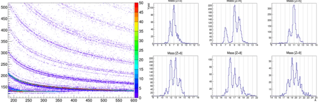
The 124Sn +64N i and 112Sn +58N i reactions were also analyzed in [3]. In this work, in which the IMFs production cross sections in semi-peripheral reactions were evaluated for dynamical and statistical emission, the previous analysis of [2] was extended by enlarging by about a factor 2 the impact parameter window of the collision toward more dissipative collisions, evaluating cross sections of the observed IMFs from atomic number Z = 3 up to Z = 22. In this case, the events were selected by requiring a PLF residue having atomic number Z >∼ 20 and parallel velocity with respect to the beam axis (in laboratory refer-ence frame) Vpar >∼ 6 cm/ns. In most of the selected events, that have reduced impact

parameter bred > 0.4, PLF has Z ∼ 45 and Vpar ∼ 7.5 cm/ns, slightly below the beam

velocity of ∼ 8 cm/ns.

In figure 1.15 the probability (panel a)) and the cross section (panel b)) associated to the multiplicity of IMF detected in coincidence with the PLF for the two reactions (124Sn +64 N i and 112Sn +58 N i) are shown (TLF residues have been excluded follow-ing the method described in Sec. II of [3]). Specifically, events with IMF multiplicity

Figure 1.15: Probality associated to multiplicity of IMF detected in coincidence with the PLF for the two reactions (124Sn +64N i (full circles) and112Sn +58N i (empty triangles)), normalized to the number of selected events, (panel a)); cross section associated to IMF multiplicity for the same systems (panel b)); ratio of the probabilies given in panel a) (panel c)) [3]. All the plots have been obtained by taking into account the detection efficiency of the experimental apparatus, using the HIPSE code [32] as event generator and a software replica of CHIMERA multi-detector [33].

equal to zero correspond to “binary events” in which, in addition to PLF-TLF binary partners, only Light Charged Particles (LCP) (Z ≤ 2) have been produced. These events are more probable in the neutron poor systems than in the neutron rich one.

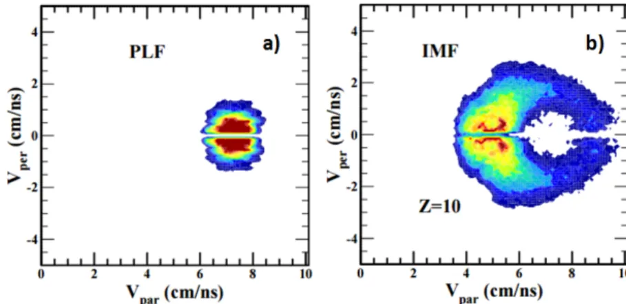
Instead, in panel c) of figure 1.15 the ratio of the two probabilities (given in panel a)) as a function of IMF multiplicity is presented. This panels clearly shows that the relative probability (neutron rich_{neutron poor}) increases with the IMF multiplicity. Thus, in order to investigate the origin of the difference in IMF emission probability between the two systems, the con-tribution of both statistical and dynamical emission mechanisms were evaluated, limiting the study to the class of events with IMF multiplicity equal to one [3]. In particular, in figure 1.16 Vpar − Vper Galilean-invariant cross-section plots for PLF (panel a)) and one

IMF of Z=10 (panel b)) for124_{Sn +}64_{N i are shown. Considering V}

par− Vper plot of IMF,

Figure 1.16: Vpar− Vper Galilean-invariant cross-section plots for PLF (panel a)) and one IMF

of Z=10 (panel b)) for124Sn +64N i reaction at 35 AM eV [3].

it’s possible to see that IMF populate preferentially the low velocity side of the Coulomb ring, which means that they are backward emitted in the primary PLF* (PLF+IMF cen-ter of mass) reference system; this is typical of dinamical emission. Moreover, a structure reminiscent of Coulomb ring, centred around the centroid of PLF parallel velocity is also present (statistical decay). To estimate the weight of the two components, also here the cos(θprox) distributions have been calculated. In particular, in figure 1.17, the dynamical

(panel a)) and statistical (panel b)) contributions to the cross section as a function of IMF atomic number for the two systems (124_{Sn +}64 _{N i and} 112_{Sn +}58 _{N i) are shown.}

It results that, while statistical emission has the same probability in both systems, the dynamical fission probability is enhanced up to a factor 1.5-2 in the neutron rich system [3]. The origin of this enhancement could be related to the entrance channel Isospin dif-ference between the two systems; but, also the different sizes of studied systems can play an important role.

Figure 1.17: Cross section associated to dynamical (upper panel) and statistical (lower panel) emission mechanism for neutron rich system124Sn(35 AM eV )+64N i (full symbols) and neutron poor one112Sn(35 AM eV )+58N i (empty symbols) [3].

1.3

Theoretical models

These studies have also motivated calculations in the framework of CoMD-II model [5] and BNV codes [34]. These models allow to describe the main features of dynamical emission and neck fragmentation.

1.3.1

CoMD-II model

The Constrained Molecular Dynamics-II (CoMD-II) model is a molecular dynamics model [5, 35] which allows to reproduce some characteristic features of the dynamical fission process. Its main feature is a self-consistent N-body approach that overcomes the main problems typically related to semiclassical many-body dynamics by solving the equations of motion using constraining procedures to satisfy the Pauli principle (event by event) and to respect the conservation rule regarding total angular momentum. This last feature plays a crucial role in producing dynamical processes with different time characteristics. In particular, the124_{Sn(35 AM eV )+}64_{N i system was investigated generating several tens}

of thousands of events with the CoMD-II model up to a maximum time of 800 f m/c and for impact parameters b ranging from 0 to 0.85bmax (bmax ≈ 10.5 f m). Comparing the

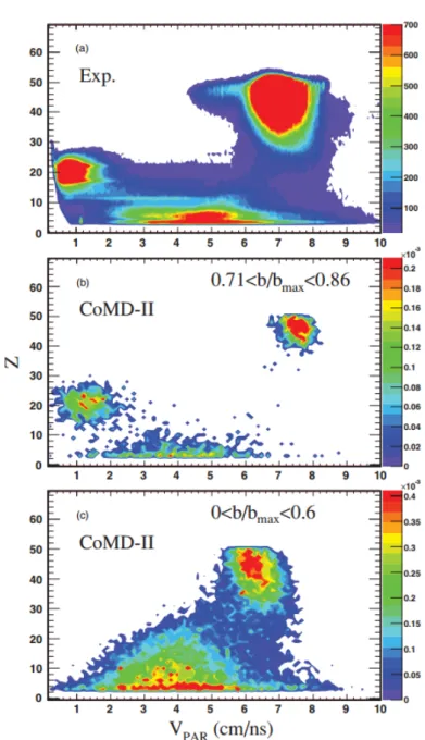
results of CoMD-II calculations with experimental data for the distribution of fragments as a function of their atomic number Z and their longitudinal velocity, it’s possible to see that these quantities are very similar (fig. 1.18). Specifically, in the upper panel of fig. 1.18 the experimental charges and velocities of the three biggest fragments with Z ≥ 3 for124_Sn+64

Figure 1.18: Experimental charge Z vs parallel velocity Vpar plot for the three biggest fragments

with Z ≥ 3 for 124Sn +64N i system (upper panel). The analogous plots evaluated with the CoMD-II model for 0.71 < b/bmax< 0.86 (panel b)) and for 0 < b/bmax< 0.6 (panel c)) [5].

N i system is presented; while, the panels b) and c) show the same distributions obtained with CoMd-II calculations for 0.71 < b/bmax < 0.86 and for 0 < b/bmax < 0.6 respectively.

Calculations indicate that the shape of such a correlation plot sensitively depends on the selected b window. In the case of smaller impact parameters (panel c) of fig. 1.18), the PLF fragment has a lower velocity, while target residue shows the charge considerably reduced and velocity increased. Thus, there is the tendency of TLF to populate a region that is usually filled by the IMFs of intermediate velocity produced by more peripheral reactions. In this case the so-called neck formation process can merge with the TLF multi-break-up. Moreover, CoMD-II calculations can reproduce the reduced relative velocity of the IMF with respect to the TLF fragment (V_redIT) as a function of its reduced velocity with respect to the PLF (VIP

red) (fig. 1.19)(VredIT and VredIP represent the relative velocities

of IMF with respect to TLF and PLF divided by the corresponding value obtained from the Viola systematics). In fig. 1.19 the comparison between experimental and theoretical

Figure 1.19: In panels a) and b) the experimental VIT

red−VredIP plots for ternary events are presented

(in panel b) only IMFs having a parallel velocity range of 2.5-5 cm/ns have been considered). Panels c) and d) show the analogous plots obtained from CoMD-II calculations. The calculation results obtained for IMFs velocities outside the range 2.5-5 cm/ns are shown in panel e) [5].

data is shown. Specifically, panel d) shows that the experimental correlations close to the mid-rapidity IMF velocities are well reproduced from CoMD-II calculation. However,

perhaps due to the finite time of the calculations, the greater yield seen in panel a) along the VIP

red = 1 axis (corresponding to a longer time scale toward the PLF fission) is not

reproduced in panel c). Nevertheless, the region along the V_redIP = 1 axis is not empty, as it’s possible to see in panel e) of fig. 1.19 where the calculated V_redIT− VIP

red plot for the IMF

parallel velocities outside of the range 2.5-5 cm/ns is shown. Specifically, the simulated events of this region include the PLF fission evolving with an average decay time of about 300 f m/c and producing an IMF with an average mass of about 35 units. About that, fig. 1.20 shows time evolution of the average mass numbers of the three biggest fragments according to the CoMD-II model for ternary (full dots) and dynamical fission events (open circles). This evolution is characterized by a “time delay” of about 130 f m/c. The TLF

Figure 1.20: Time evolution of the average mass numbers of the three biggest fragments according to the CoMD-II model for ternary (full dots) and dynamical fission event (open circles). A1, A2,

A3 indicate PLF, TLF and IMF respectively [5].

(A2) is formed after about 50 f m/c and the PLF (A1) undergoes a binary splitting in

the subsequent time interval of about 300 f m/c. According to this study and also to the result obtained in Ref.[10], in ternary events, for moderate asymmetry between the masses of PLF and IMF produced at mid-rapidity, a large contribution is given from a dynamical sequential breaking of the hot PLF. These events also show a Φplanedistribution

strongly peaked at forward angle. In particular, the average value of Φplane (Φplane) allows

to have information related to the characteristic time of the process. In fig. 1.21 a comparison between the experimental Φplane distribution for 124Sn +64N i system (open

Figure 1.21: A comparison between the experimental (open circles) and calculated (full circles) Φplane distribution for events with AH/AL< 5 and VparL > 3 cm/ns [5].

reproduce the experimental Φplane distribution well, including the background associated

with the primary PLF splitting processes with longer emission times; this almost flat contribution is related to the statistical emission. CoMD-II calculations was also used to investigate the difference in dynamical fission strenght between the neutron rich and the neutron poor system seen in the REVERSE experiment. As said previously, during this process the PLF breaks in two main fragments, AH (the heavy one) and AL(the light one),

whose ratio is named AHL. Experimental data obtained during the REVERSE experiment

show that the yield of processes related to the dynamical PLF fission is higher for the neutron-rich system with respect to the case of the neutron-poor one. This difference could be related to the entrance channel Isospin difference between the two systems; but, it could also be due to their different sizes. In order to disentangle these two effects, the AHL (AH/AL) distributions predicted by CoMD-II model for the two systems (124Sn(35

AM eV )+64_{N i (red line) and}112_{Sn(35AM eV )+}58_{N i (blu line)) were compared with those}

of the124_{Cs(35 AM eV )+}64_{Ga system [4]. This system has the same mass of neutron-rich}

system (124_{Sn +}64_{N i) and N/Z ratio equal to the neutron-poor one (}112_{Sn +}58_{N i). As it’s}

possible to see in fig. 1.22, where the AHL distributions for the three systems are shown,

the 124Cs +64 Ga system (light blue line) present a AHL distribution similar to the one

measured for the neutron rich reaction (124Sn +64N i). So, CoMD-II model suggests that the origin of the observed difference is related to the entrance channel mass difference of the two systems.

Figure 1.22: AHL distributions for three systems: 124Sn +64N i (red line), 112Sn +58N i (blu

line) and124Cs +64Ga (light blue line) [4].

1.3.2

BNV stochastic transport model

The Boltzmann-Nordheim-Vlasov stochastic transport model is a stochastic mean field microscopic apporach that describes via a transport equation the time evolution of the nucleon one-body distribution function in phase space f (~r, ~p, t) [36, 37]. It provides a generally good average description of the dissipative mechanisms occurring all along the interaction between the two colliding nuclei. According to entrance channel properties, different out-coming channels, from the formation of only one composite nuclear source (in the case of central collisions) up to deep-inelastic-like processes (in the case of peripheral reactions), are observed [36, 37]. In particular, Baran et al. [34] investigated fast fragments production mechanism from semi-central to peripheral collisions (bred= b/bmax≥ 0.37) for

the 124_{Sn(35AM eV )+}64_{N i and} 112_{Sn(35AM eV )+}58_{N i systems. They used a BNV [34]}

approach to mean field with a stochastic fluctuating term that takes into account dynamics of fluctuations. The transport equations are solved following a test particle on lattice. In the collision term, a parametrization of free nucleon-nucleon (NN) cross section is used, with energy and angular dependence. Moreover, the isospin effects on the nucleon cross section and Pauli blocking are consistently evaluated. Events observed in the calculation were divided in three classes:

1. binary events with excited TLF* and PLF* that, having small deformation, remain so for long times. Their sequential decay can be described by statistical models; 2. binary events in which especially PLF* have large quadrupole or octupole

deforma-tion;

there is an IMF directly emitted in less than ∼ 250 f m/c from the reaction beginning. Fig. 1.23 shows the scatter plot of freeze-out quadrupole versus octupole moment for all fragments of events of the first two classes for different impact parameter values. In this figure it’s possible to distinguish two branches that can be associated to deformed PLF* (left branch) and TLF* (right branch). The large dynamically induced

deforma-Figure 1.23: Scatter plot of freeze-out quadrupole versus octupole moment for all fragments of the events of the classes (1) and (2) for different impact parameter values [34].

tions can drive especially the PLF* towards a fast asymmetric fission. The corresponding signs suggest pear-shaped fragments oriented with the smaller deformation towards the separation point. The last two classes of events can contribute to the “dynamical” pro-duction of IMFs. Instead, in fig. 1.24 typical evolution of the density contour plot for a ternary event (event of class (3)) at b = 6 f m for the system 124_{Sn(35AM eV )+}64_{N i is}

shown. Initially, for the first 20-60 f m/c the two participants deeply interact and at this time some compression takes place. The system heats up and a relative expansion fol-lows. Despite its compact form, the system still behaves as a “two-center object” with an effective superimposed separate motion of the PLF and TLF pre-fragments. This motion induces the formation of a neck-like structure that, between 40 f m/c and 140-160 f m/c, rapidly changes geometry, depending on the impact parameter. After about 150 f m/c, this neck-instability dynamic favors the emission of IMFs. Their production probability depends on the impact parameter, as shown in fig. 1.25; it’s maximal (around 25%) for semiperipheral collisions (b=6-7 f m), while it strongly decreases for semicentral (b=4-5 f m) collisions and at larger impact parameter, where this mechanism is suppressed by a less overlapping and a faster separation. Moreover, fig. 1.26 presents the asymptotic frag-ment velocity distributions in the laboratory frame for all impact parameters and for all the events (binary (classes (1) and (2)) and ternary (class (3)) events) of the three classes; in this plot “vpar” is the velocity component along the beam direction while “vtran” is the orthogonal part. The IMFs are found in relatively wide midrapidity region, in strong

Figure 1.24: Typical evolution of the density contour plot for a ternary event (event of class (3)) at b = 6 f m for the system124Sn(35AM eV )+64N i [34].

Figure 1.25: The impact parameter dependence of the probability for ternary events in neutron-rich (white circles) and neutron-poor (black squares) reaction [34].

agreement with experimental vpar velocity distribution of fig. 1.2. Finally, in fig. 1.27 the

Figure 1.26: The asymptotic fragment velocity distributions in the laboratory frame for all impact parameters and for all fragments observed in binary events (upper panel) and ternary events (bottom panel) [34].

correlation between relative velocities Vrel/VV iola(IMF,PLF) (r) and Vrel/VV iola(IMF,TLF)

(r 1) obtained in BNV simulation for all IMFs is shown. Comparing these results with the experimental relative velocities correlation and Vpar plots (fig. 1.5 and fig. 1.2), it’s

possible to see a strong qualitative agreement expecially for lighter IMFs (ZIM F s = 4, 8).

Also this analysis supports a fast neck break-up mechanism triggering the formation of a light IMF (Z <∼ 10), localized in the mid velocity region. Moreover, in BNV simula-tion, IMFs formation is observed mainly between 140 and 260 f m/c in agreement with the results obtained with the relative correlation method (sect. 1.1). In fact this method demonstrates that light IMFs emission takes place at 40-80 f m/c after the system starts to re-separate that corresponds to about 140-180 f m/c in BNV calculation (in this case re-separation between PLF and TLF takes place around 100 f m/c). The relative correla-tion method also predicts heavy IMF emission at times of about 120 f m/c or longer after the beginning of reseparation (sect. 1.1). But, unlike the light IMFs, these events are not predicted by BNV calculation; it can’t reproduce this delayed mechanism because of a problem of instability with increasing time. However, with the events of class (2) also BNV model supports the idea of a fast neck induced fission in competition with statistical decay of primary fragments.

Figure 1.27: Relative velocity correlation plot obtained in BNV simulation for

124_{Sn(35AM eV )+}64_{N i reaction [34].}

1.4

InKiIsSy experiment: open question

The InKiIsSy experiment was carried out at Laboratori Nazionali del Sud in April 2013 in order to disentangle entrance channel isospin effects from the possible dependence of these results upon the initial different mass of the two systems. During this experiment the124_{Xe +}64_{Zn reaction was studied at 35 AM eV beam energy, it has the same mass of}

the neutron rich system (124_{Sn +}64_{N i) and a N/Z ratio close to the value of the neutron}

poor one (112Sn +58N i). During the InKiIsSy experiment also the 124Xe +64N i system was analyzed, in order to compare two systems (124Xe +64Zn and 124Xe +64N i) with same mass and beam but with different N/Z ratio for the target.

Table 1.6: Isospin values of the systems analyzed during the REVERSE (124Sn +64 N i and

112_{Sn +}58_{N i) and the INKIISSY (}124_{Xe +}64_Zn,124_{Xe +}64_{N i) experiments.}

System N/Z projectile N/Z target N/Z compound

124_{Sn +}64_{N i 1.48 1.29 1.41}

124_{Xe +}64_{N i 1.30 1.29 1.29}

124_{Xe +}64_{Zn 1.30 1.13 1.24}

112_{Sn +}58_{N i 1.24 1.07 1.18}

In tab.1.6 the value of Isospin of the four systems (REVERSE + InKiIsSy) are reported. This last measurement was performed using the multi-detector CHIMERA coupled for the first time with 4 telescopes of FARCOS array [38].

Experimental setup

In this second chapter the experimental setup used during the InKiIsSy experiment will be described. This experiment has been performed on April 2013 at the INFN-LNS in Catania by using the 4π CHIMERA multi-detector, coupled to a prototypes of the correlator FARCOS.

2.1

CHIMERA multidetector

CHIMERA (Charged Heavy Ion Mass and Energy Resolving Array) is a multidetector with high granularity and large covering of the total solid angle (94%), designed to study heavy-ion collisions in the Fermi and low energy regimes [15]. It can be schematically described as a set of 1192 detection cells arranged in 35 rings following a cylindrical geometry along the beam axis. The whole apparatus, schematized in fig. 2.1, has a total length of about 4 m and it operates under vacuum. The mechanical structure can be essentially divided into two differently shaped blocks. The forward one, covering polar angles between 1o and 30o, is made of 688 modules assembled in 18 rings, grouped in couples, and supported by 9 wheels centred on the beam axis (fig. 2.2). Each wheel is divided into 16, 24, 32, 40 or 48 trapezoidal cells, depending on its polar coordinate, containing each one a detection module, or telescope, that will be described afterwards. The rings of telescopes are placed at different distance from the target: the first ring is placed at a distance of 350 cm, while the last ring is placed at a distance of 100 cm from the target. Thus, placing telescopes at distance that increases with decreasing polar angle, it’s possible to obtain a precise measure of time-of-flight also for forward emitted fragments, that are the faster ones, being mainly emitted by the PLF. The second block, instead, is made of 504 modules grouped in 17 rings and covers the remaining angular range, between 30o_{and 176}o_{. These 17 rings are assembled in a sphere of 40 cm in radius as shown in figure}

2.3. Specifically, 15 of the 17 rings are segmented into 32 cells while the 2 backward ones are

Figure 2.1: Schematic picture of the CHIMERA apparatus.

segmented into 16 and 8 cells respectively. Each module of this spherical structure consists in a steel box containing the Caesium Iodide crystal with the silicon detector placed at the side facing the target. In table 2.1 the main geometrical characteristics of CHIMERA

Figure 2.3: A photo of the sphere of CHIMERA multidetector.

array are given. The large number of telescopes and the geometrical configuration give to CHIMERA a high granularity, thus reducing the multi-hit probability, and a high solid angle coverage, about 94% of 4π; these features, in addiction to low energy detection threshold, allow to obtain a complete event recostruction.

2.1.1

The telecopes of CHIMERA array

The basic detection module of CHIMERA array is a telescope composed by two de-tection stages: a Silicon detector (Si) with a thickness of about 300 µm, followed by a Caesium Iodide Thallium activated scintillation detector (CsI(Tl)) (fig. 2.4), coupled to a photodiode [15]. As well known, silicon is a very widely used material for nuclear physics detectors because of good energy resolution, high density (2.33 g/cm3), low energy needed to create an electron-hole pair (3.6 eV with respect to 30 eV in gases), fast signal col-lection (10 ns in 300 µm of thickness) and good time resolution. The silicon detectors used in CHIMERA have a trapezoidal shape and were made by using the planar technol-ogy [39]. This tecnique allows to have well defined detector thickness, very sharp active zones, extremely thin (500 ˚A) and homogeneous junction. Moreover, a 300 ˚A aluminium layer covers front and rear face of the silicon slice in order to ensure a good electrical contact. This characteristic slightly decreases the energy resolution because introduces a

Table 2.1: Geometrical characteristics of the CHIMERA array. For each detector of a ring, the distance from target, minimum and maximum polar angle, number of modules, azimuthal angle range and covered solid angle are specified.

dead layer; however, it gives a better overall timing performance [40] because the rise time becomes nearly independent of the impact point of the detected particles. These silicon detectors have a geometry that changes according to the position in the device while the thickness is the same (except for the Silicon detectors of first wheel that have an average thickness of 220 µm) and chosen to optimize the combined ∆E-E+∆E-TOF techniques, that will be explained afterwards. In the wheels, the forward part of the apparatus, each cell contains two telescopes, and thus two silicon detectors (internal and external detec-tors) that are characterized by the presence of two active zones in the same Silicon pad, working independently of each other. In figure 2.5, presenting a schematic rapresentation (a) and a photo (b) of wheels silicon detector, it’s possible to distinguish the two active zones and the 500 µm wide dead zone of the edge of the detector; moreover, a guard ring is placed in this dead zone around the two pads at a distance of 50 µm from the edges of the active area. The 504 Si detectors of the sphere (figure 2.6), are simple pad detector;

Figure 2.5: A schematic view (a) and a photo (b) of a wheels silicon detector.

even in this case a 500 µm dead zone, in which a guard ring is placed, surrounds the active area. The second stage of CHIMERA’s basic module consists of Caesium Iodide Thallium activated crystals CsI(Tl). These scintillators are used to measure the residual energy of particles that punch through the silicon detector [41]. The shape of CHIMERA’s crystals is a truncated pyramid with a trapezoidal base; the dimensions of front surfaces are the same of the silicon detector ones and depend on the position in the device. The backward surface is bigger than the front one, depending on the thickness of the crystal that ranges from 3 (at backward angles) to 12 (at forward angles) cm.

Figure 2.6: A photo (a) and a schematic view (b) of the sphere silicon detectors.

This kind of crystal is chosen as second stage detectors because of its high density, since the high stopping power allows to reduce the thickness needed to stop high energetic light charged particles. Furthermore, they are characterized by relatively low cost, simple han-dling, a good resistance to radiation damage, good light output performance when coupled with a photodiode or a photomultiplier, and offer the ability to get an isotopic identifi-cation through the Pulse Shape Discrimination (PSD) technique, which will be described afterwards. A disadvantage of these scintillators is the non-linearity (at low energies) in light response, that is, light output is therefore not directly proportional to the deposited energy, depending on the ionizing power of the fragment. The CsI(Tl) crystals, in the case of CHIMERA array, are coupled with photodiodes (PD) [42, 43] that, with respect to photomultipliers, are favourites for their low operating voltage (low power dissipation), simple handling and compact assembly under vacuum. The photodiodes, manufactured by Hamamatsu Photonics, are 300 µm thick with an active surface of 18×18 mm2 _{and are}

encapsulated in a ceramic support with the front side (corresponding to the light entrance surface) protected by a thin window of transparent epoxy resin.

2.2

Electronic chain

The signals from Silicon detectors and CsI photodiodes are handled by two different electronic chains that process and digitize the signals so that they can be read by the acquisition system. These electronic chains were designed to satisfy some important re-quirements: a large dynamic range (from M eV to GeV ), a good timing in order to reach a resolution better than 5% (the exact time resolution depends on velocity and base of flight) in velocity measurements through the TOF technique, a low power dissipation under

vac-uum, a high level of flexibility in coupling the detector with other experimental devices and a good energy resolution. The preamplifiers (PA) of silicon detectors and photodi-odes are placed on motherboards inside the vacuum chamber in order to reduce electronic noise and signal losses in parasitic circuits, that strongly affect the energy resolution. The number of the preamplifiers placed on a motherboard is not equal for the wheels and the sphere. In fact, in the forward part, each motherboards contains four preamplifiers, two for the internal telescope and two for the external one (each telescope needs two PACs, one for the silicon and one for the photodiode). In this case the motherboards are located on the external surface of the wheels. Instead, the motherboards in the sphere have only two preamplifiers, corresponding to only one telescope, and are located on the top of the metallic baskets containing the telescopes (fig. 2.7). All the motherboards are cooled, using a refrigerating liquid circulation, in order to assures the stability of the electronic against the power dissipation. The voltage generators for detectors and preamplifiers with the rest of the electronic chain are placed outside the vacuum chamber.

Figure 2.7: Photos of the motherboards for sphere detectors (a) and for wheels detectors (b).

2.2.1

The electronic chain of silicon detectors

The first stage of the electronic chain of silicon detectors is a charge preamplifier designed to perform good timing measurements coupled to high capacitance detector, providing a first amplification of signal. It integrates the detector signal giving an output independent of detector capacity and proportional to the charge produced by the detected particles. Each preamplifier has a test input which accepts signals coming from a pulse generator in order to control the electronic stability. The output is a single negative fast signal carrying time and energy information, with a rise time of ≈ 50 - 200 ns and a decay time of ≈ 200 µs. The preamplifier sensitivity changes with changing of the polar angle: in

the most forward rings (θ=1o _{÷ 10}o_{), where the more energetic particles are expected, the}

sensitivity is 2 mV /M eV , while in the rest (θ=10o _{÷ 176}o_{) it is 4.5 mV /M eV . In the first}

period of CHIMERA operation (before 2008), the second stage of the electronic chain was a CAMAC 16 channels bipolar amplifier. Each channel of amplifier produced a negative front bipolar signal (with the positive side ‘cutted’) as energy output and an unipolar timing output differentiated to 100 ns and integrated to 20 ns. It was also possible to use the multiplex output to observe the signals. Then, the energy signal is coded by a Charge-to-Digital Converter (QDC). Specifically, the conversion of the signal can be “High Gain” (HG) or “Low Gain” (LG). In the first case an amplification factor 8× is applied for low energy signals. Instead, timing logical signals for the silicon detectors are generated by a high resolution Constant Fraction Discriminator (CFD). Each discriminator presents:

• an input signal with 50 Ω impedance and maximum amplitude of 5 V ; • a delay of 20 ns;

• a typical fraction of 30 %;

• a variable discriminator threshold from 1 to 256 mV in step of 1 mV ; • an automatic set of the walk.

In particular, the discriminator provides two output analogical signals: a prompt out-put used as a start signal for a VME 9U Time-to-Digital Converter (TDC), and a delayed one that, together with an OR output signal, is sent to the trigger control system. The stop signal is then provided by Radio Frequency (RF) of the Cyclotron and sent to the same TDC that gives a 12 bit value proportional to the temporal distance between the start and the stop signals. In figure 2.8 a sketch of the basic electronic chain of silicon detectors is shown. In the last years, substantial changes have been introduced in the elec-tronic chain in order to allow the application of the pulse shape tecnique also to the silicon detectors (described in section 2.4.4). In fact, from ring 4 to ring 13, the old CAMAC elec-tronics has been replaced by new compact modules particularly studied to measure also the rise time of the silicon signal; in this way it’s possible to get the charge of particles stopped in the silicon detectors [44, 45]. In particular, in order to measure the rise time of the Silicon signal, a new compact NIM module, coupling an amplifier with two different discriminators characterized by different fraction, 30% and 80%, has been adopted. Two copies of the PA signal are differentiated by 50 and 500 ns and sent, respectively to two CFD with 30% fraction-30 ns delay and 80% fraction-150 ns delay. The CFD outputs are used as start signals of two TDC channels, both receiving as stop signal a delayed copy of the RF signal. By means of the difference between the two TDCs’ outputs, T30% and T80%

Figure 2.8: Block diagram of the basic front-end electronics of silicon detectors.

respectively, it’s possible to obtain the rise time of the signal. Specifically, considering that true values of T30% and T80% are equal to:

T_30%T rue = Tstop− T30%M easured (2.1)

T_80%T rue = Tstop− T80%M easured, (2.2)

the rise time of the signal will be:

Trise = T80%T rue−T30%T rue = Tstop−T80%M easured−(Tstop−T30%M easured) = T30%M easured−T80%M easured. (2.3)

In figure 2.9 the new configuration with the amplifier and the two different discrimi-nators is schematized (red box).

2.2.2

The electronic chain of CsI(Tl) crystals

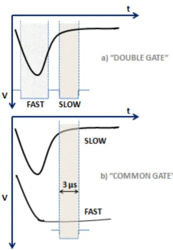
The signal from the CsI(Tl) detector firstly is processed by a charge preamplifier that presents the same characteristics of those used for Si detectors, except for the sensitivity that is of the order of 50 ÷ 100 mV /M eV (Si-equivalent). The rise time of output signals is significantly longer than 50 ns and can reach values of 1-2 microseconds. The output signal is sent to a unipolar amplifier that amplifies and shapes it with variable shaping time (0.5, 1, 2, 3 µs). These amplifiers, assembled in a 16 channel NIM module, have a double output in energy for each channel, with different gains (the higher one is 10 times the lower one) but equal shaping time (∼ 2 µs) and a fast timing output with gain 15. The two well shaped energy amplifier outputs follow two separate lines (see fig. 2.14): the higher

Figure 2.9: Upgrade of the silicon detectors’ electronic chain (in dashed box) for the pulse shape technique.

one is sent to a QDC for the integration of the so called slow CsI(Tl) signal component, while the lower one is stretched by a 48 channel module and then sent to another QDC for the integration of the fast signal component (see section 2.4.2). In particular,a stetcher is used in order to avoid the insertion of delays and the effects of jitter in the integration of signals with respect to the common gate.

Figure 2.10 shows a schematic view of the electronic chain of CsI(Tl) coupled with a photodiode (PD). Then, a Data Acquisition System ([46, 47, 48, 49, 50, 51]) is needed that allow a fast overview of growing physical results, in order to collect and store data coming from both Silicon and CsI(Tl) electronic chains.

2.3

FARCOS array

During the InKiIsSy experiment, for the first time, CHIMERA was coupled with 4 telescopes of FARCOS (Femtoscope ARray for COrrelations and Spectroscopy) array [38]. Its main peculiarities are the good energy and angular resolution and the high modularity. Specifically, during this experiment, 4 FARCOS telescopes were placed at 25 cm from the target, subtending the polar angles 15o _{≤ θ}

lab ≤ 45o and an azimuthal interval ∆φ ≈ 90o.

They were used to measure, with better angular resolution than in CHIMERA, IMF and Light Charged Particles.

Figure 2.10: The front-end electronics of CsI scintillator.

Figure 2.11: A sketch view (left panel) and a photo (right panel) of the 4 telescopes of FARCOS array placed at 25 cm from the target (15o≤ θ_lab ≤ 45o_{, ∆φ ≈ 90}o_{) inside CHIMERA sphere.}