1
Tax Liability Side Equivalence and Time Delayed Externalities
*Lingbo Huang Department of Economics
Monash University (AU) Email: [email protected]
Silvia Tiezzi
Department of Economics and Statistics University of Siena (I)
Email: [email protected] Erte Xiao
Department of Economics Monash University (AU) Email: [email protected]
December 2018
Abstract
Past experimental research suggests that taxes levied on the buyer side are sometimes perceived as more acceptable than equivalent taxes levied on the seller side, violating the well-known Tax Liability-Side Equivalence Principle. This paper tests whether the statutory incidence of the tax mitigates the negative impact of delayed externality on public support for Pigouvian taxation. We show that the delay effect is robust regardless of the side the tax is levied on and regardless of whether buyers display a tax shifting bias.
JEL codes: D03, D62, D72, H23
Keywords: tax liability side equivalence, externalities, support for taxation, intertemporal choice
* We gratefully acknowledge the Australian Research Council Discovery Project (DP160102743) for funding this research. We thank participants at the 9th Southern European Experimental Team (SEET) Workshop, Lecce (I) 23-25 February 2018 for useful comments.
2 1 INTRODUCTION
A major impediment to the introduction of efficiency-enhancing Pigouvian taxes, such as a carbon tax, is their low public support. While general distaste for taxation may explain low support for Pigouvian taxes,1 an important feature of climate change related taxes is that their benefits (e.g. clean air) are only experienced some time after the tax is paid.
Tiezzi and Xiao (2016) provide experimental evidence that consumers are generally less willing to support a taxation policy aimed at reducing consumption externalities when the latter occur some time after consumption. In that study, the tax was imposed on the demand side. In practice, however, carbon taxes are seldom levied on consumers. For example, in the EU Emission Trading System (ETS), the existing carbon pricing schemes are often imposed on large industrial point sources of emissions. This raises the question whether the delay effect persists when the tax is levied on sellers.
The Liability-Side Equivalence Principle (LSE) establishes that the economic incidence of a tax, i.e. who ultimately bears the burden of the tax, is independent of the side of the market the tax is levied on, implying that public attitudes to taxation are not affected by the side of the market that is taxed.
Experimental studies on LSE have produced mixed results. One strand of literature shows that the LSE holds both in competitive (Kachelmeier, Limberg and Shadewald 1994; Ruffle 2005) and non-competitive markets (Riedl and Tyran 2005; Menges and Traub 2008).
Another group of experimental studies finds, in different economic environments, no evidence of liability side equivalence (Kerschbamer and Kirchsteiger 2000; Cox, Rider and Sen 2017; Morone, Nemore and Nuzzo 2016; Weber and Schram 2017). Finally, Sausgruber and Tyran (2005, 2011) conduct experiments similar to ours and observe that buyers prefer an inefficiently high seller tax to an efficient buyer tax (tax-shifting bias). The existence of a tax-shifting bias opens up the possibility for policy makers to increase public support for taxation by exploiting that bias in designing new tax institutions (Gamage and Shankske 2011; Schenk 2011)2. None of the above studies investigates the existence of the tax-shifting bias in an intertemporal setting with
1 Such as distrust in government (Rivlin 1989; Dresner et al. 2006); worldviews (Cherry, Kallbekken, and Kroll 2017); and tax aversion (Kallbekken, Kroll, and Cherry 2010; Blaufus and Möhlmann 2014).
2 Aside from these framing effects, there are other reasons for preferring a supply side tax over a demand side tax, as reported among others in Collier and Venables (2014), Lazarus et al. (2015) and Metcalf and Weisbach (2009).
3
real time delays. Time-delayed externalities (i.e. externalities that produce their effects only after
some time) add another dimension that may affect participants’ preferences for taxation, besides the statutory incidence of the tax. This raises the second question of whether levying the tax on sellers could mitigate the negative effect of the delayed benefit on support for Pigouvian taxation.
To answer both questions we conduct an intertemporal market experiment on public support for taxes (Kallbekken, Kroll, and Cherry 2011; Sausgruber and Tyran 2005; Cherry, Kallbekken, and Kroll 2017; Tiezzi and Xiao 2016). Participants can earn money by purchasing a hypothetical consumption good in their market. Consumption, however, imposes a negative cost on everyone in the market. We manipulate the timing of the externality and introduce opportunities for buyers to vote on whether to introduce a tax on consumption. The experiment adopts a two by two design. The two treatment variables are whether the externality is delayed (No delay vs. Delay) and whether the tax is levied on the demand or on the supply side of the market (Buyer tax vs. Seller tax).
We first identify whether under our No delay baseline condition, participants display a tax-shifting bias. We find no evidence of tax-tax-shifting bias when the whole data sample is used. When the data is split by gender, female, but not male buyers display a tax-shifting bias. In the Delay condition, irrespective of the gender, we find a strong Delay effect. The negative delay effect on support for taxation remains strong even when the tax is levied on sellers, regardless of whether the participants display a tax-shifting bias or not. This highlights the importance of the timing of the tax benefits in attitudes towards taxation.
2 EXPERIMENTAL DESIGN
We first replicate the delay effect reported in Tiezzi and Xiao (2016) in which the tax is levied on buyers. The two Buyer tax treatments (BuyerTax_NoDelay and BuyerTax_Delay) are basically the same as the Delay and No Delay treatments in that paper (more detail on the rationale of some design specifics can be found in Tiezzi and Xiao, 2016). Then we describe the two new treatments where the tax is levied on sellers.
2.1 Buyer tax treatments
The treatments are based on a simple uniform-price, multi-unit auction market with externalities. A market consists of four buyers and one automated seller. Buyers earn money by trading up to
4
three units of a hypothetical consumption good in their market. They are informed of the resale value of each unit (160, 110 and 70 points, respectively) and told that the seller’s marginal cost remains constant throughout the experiment. When an auction starts, each buyer posts a bid for each of the three units and the bid for a unit is capped at its resale value. Sellers have a per-unit production cost of 40 points (unknown to buyers). Sellers accept all bids greater than or equal to the per-unit production cost and all accepted units are sold at the market price (the lowest accepted bid). Each buyer’s gross income for each purchased unit equals the difference between its resale value and the market price. Units that are not traded yield zero income.
Each traded unit generates an external cost of 60 points shared equally by all buyers in the market. That is, regardless of who gets the unit, each buyer in that market bears a cost of 15 points. We manipulate the timing of the externality. In the BuyerTax_NoDelay treatment, the costs are deducted immediately from the current earnings collected at the end of the session. In the BuyerTax_Delay treatment, the external costs are deducted from the buyers’ future earnings (an endowment of $18) to be collected one week later. This is the only difference between the two treatments.
This market is repeated for two practice periods and ten paying periods. At the end of each period, participants receive full history feedback including the market price, market quantity, their bids, per-capita external costs, per-period earnings and accumulated earnings for the day of the experiment and one week later. The values of the parameters are designed so that at market equilibrium (Delay or No Delay), all buyers purchase all three units at price of 40 points, although the socially optimal outcome is when every buyer only purchases two units. In particular, as shown in Tiezzi and Xiao (2016), this equilibrium holds in the Delay condition unless buyers have extremely high discount rates (i.e. annual discount rate higher than 100%).
Unbeknownst to the participants, before the start of the 11th period, we introduce a Pigouvian tax and a voting mechanism to buyers’ decisions. The tax is revenue neutral: a tax of 60 points (equal to the per-unit external cost) for each traded unit is imposed on either buyers or sellers; then an equal share of the total tax revenues is returned to each buyer.
In the ballot, all participants simultaneously vote yes or no on the introduction of the tax; abstentions and neutral votes are not possible. The tax is implemented in a market for the following trading periods if at least two buyers in the market vote yes. After all buyers cast their votes,
5
acceptance or rejection of the tax is revealed, though individual votes are kept secret. The tax regime is effective for the next five periods (11th to 15th).
In addition to voting yes or no, we assess the degree of support by asking participants to choose one from the following eight options: Don’t Know; Indifferent; Somewhat Yes (No); Moderate Yes (No); Strong Yes (No). In the 16th period, all buyers are again prompted to vote on the tax and declare their degree of support. The outcome of the second ballot is effective for the final five periods (16th to 20th).
2.2 Seller tax treatments
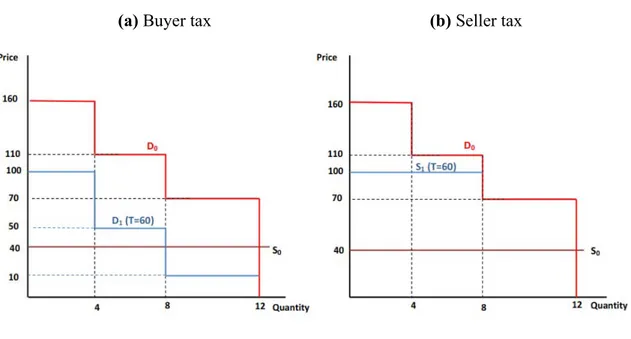
The two Seller tax treatments differ from the Buyer tax treatments only in that buyers are told that the tax is imposed on the sellers. Specifically, buyers are told that if the tax is introduced, sellers’ production cost for each traded unit increases by 60 points. The right panel in Figure 1 shows the implication of buyer and seller taxes on market equilibrium. The left panel shows that the tax shifts the demand function down from D0 to D1. The right panel shows that the tax shifts the supply
function up from S0 to S1. In both cases, the socially optimal outcome is reached with taxes at market equilibrium.
Like the two Buyer tax treatments, the SellerTax_NoDelay treatment differs from the SellerTax_Delay treatment in that the external costs are immediately paid in the No Delay condition, while they are delayed and deducted from earnings one week later in the Delay condition.
We emphasize that both types of taxes are transaction taxes depending only on the number of units traded, not on their resale values. The tax rates are also the same, regardless of whether the tax is levied on buyers or sellers. Thus the expected profit for buyers is the same regardless of the liability side of the market. Hence, Tax Liability Side Equivalence holds at market equilibrium.
6
Figure 1: Induced market demand and supply (a) Buyer tax (b) Seller tax
2.3 Procedure
At the beginning of a session, participants were randomly assigned to markets and remained in the same market throughout the experiment. The first set of instructions for the two practice periods and the first ten trading periods was distributed to participants in paper form and read aloud by the experimenter. Participants were not informed about the voting stage until they reached the end of the 10th trading period, when the second set of instructions was distributed and again read aloud by the experimenter. To ensure that participants understood the instructions, they were asked to answer a comprehension quiz after reading each set of instructions. A post-experiment questionnaire was administered at the end of the 20th period.
To manipulate the timing of the externality and the benefit of the tax, we told participants at the beginning of the experiment that in addition to accumulated earnings from trading, they would receive an additional $18 cash payment minus costs incurred in the experiment exactly one week later. To receive this additional money, participants had to return to the lab exactly one week after the end of the experiment; on that occasion they did not have to perform any additional task. To minimize any credibility concerns on money collection, at the end of each session, participants each received a “payment certificate” signed by the experimenter. The certificate indicated the amount to be received, the date, time and location for collection of the payment, and the contact details of the experimenter, including office address, telephone and email address. The day before
7
the scheduled pickup, participants received an email reminder.3 The timeline of the experiment is illustrated in Figure A.1 of Appendix A.
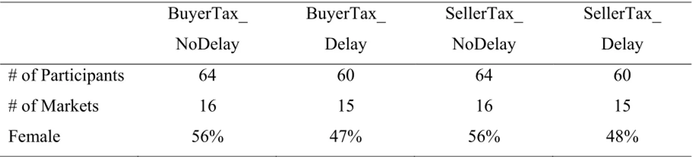
Table 1: Experimental treatments and gender ratio BuyerTax_ NoDelay BuyerTax_ Delay SellerTax_ NoDelay SellerTax_ Delay # of Participants 64 60 64 60 # of Markets 16 15 16 15 Female 56% 47% 56% 48%
Sixteen computerized sessions programmed in z-Tree (Fischbacher 2007) were conducted at the Monash Laboratory for Experimental Economics (MonLEE) with a total of 248 participants (52% female). Each participant could only participate in one of the four treatments. Table 1 shows the number of participants and gender ratio by treatment. Earnings were expressed in experimental points and exchanged for cash at $1(Australian dollars) per 200 points.A typical session lasted around 2 hours with 16 or 20 participants earning on average $28 including a $5 show-up fee. All instructions are reproduced in Appendix B.
3 RESULTS
Buyers’ voting decisions, which revealed their tax attitude, were the main variable of interest. We also obtained data on buyers’ degrees of support. This additional data revealed finer details of changes in attitudes towards the tax. Degree of support was rated on a 7-point scale from 0 (Strong No) to 6 (Strong Yes).4 We first tested for tax-shifting bias under No Delay baseline conditions. Only female buyers showed bias in the first ballot. We then examined the negative delay effect on support for the seller tax, separately for females and males. We began with the inexperienced voters in the first ballot and then examined behaviour in the second ballot to shed light on the effects of learning from experience.
3 To minimize any transaction costs implied by going back to the lab, participants were given the possibility of rescheduling the pickup time or pickup day. Participants could also send someone else on their behalf, to pick up their second payment.
4 We also allowed participants to select “Don’t Know”. Only eight buyers chose this option. We excluded these eight buyers when analyzing degree of support.
8
3.1 Support for tax-shifting bias under No Delay conditions
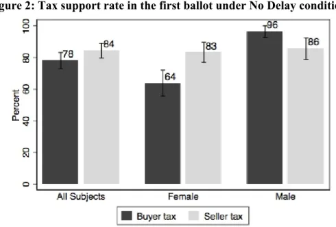
Figure 2 shows the average tax support rate (the proportion of Yes votes) and Figure 3 plots the distribution of degree of support in the first ballot under No Delay conditions. Error bars represent one standard error of the mean.
Figure 2 shows that the average support rate for the seller tax was slightly higher than for the buyer tax. Although the direction was consistent with the tax-shifting bias, it was not statistically significant (78% vs. 84%, Z-test, one-tailed p = 0.183).5 When we broke down the data by gender, however, we found that female, but not male, voters showed tax-shifting bias.
As shown in Figure 2, among female voters, the average support rate for the seller tax was significantly higher than the support rate for the buyer tax (83% vs. 64%, Z-test, p = 0.031). The degree of support suggested even stronger evidence for tax-shifting bias: the average degree of support was significantly higher for the seller tax than for the buyer tax (4.68 vs. 3.68, t-test, p = 0.005). The distribution of the degree of support shown in Figure 3 provides additional information on changes in attitudes. First, we note that the number of participants who responded “Indifferent” was small. This means that most participants did hold a view, either positive or negative, about the tax. Second, none of the Yes voters chose Somewhat, Moderate or Strong No and none of the No voters chose Somewhat, Moderate or Strong Yes. This means that degree of support data was consistent with voting. Comparing the degree of support among Yes voters, we found that the main difference between the buyer tax and the seller tax was that a relatively higher proportion of females expressed Strong Yes (score 6), while no participant expressed Moderate or Strong No (scores 1 and 0) to the seller tax.
9
Figure 2: Tax support rate in the first ballot under No Delay conditions
Figure 3: Distribution of degree of support in the first ballot under No Delay conditions
In contrast, we did not find any evidence of tax-shifting bias for male voters. The average support rate for the seller tax was even slightly lower than for the buyer tax and the difference was not significant (86% vs. 96%, Z-test, p = 0.920). Nor did the average degree of support differ significantly between the two tax frames (4.41 vs. 4.93, t-test, p = 0.936). The distribution of degree of support plotted in Figure 4 shows that most male voters expressed some degree of support for both the buyer tax and the seller tax.
As only female voters showed tax-shifting bias, we then compared the delay effect on the buyer and seller taxes separately for female and male voters.
10
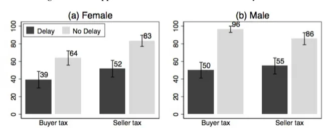
3.2 Delay effect and support for seller tax vs. buyer tax
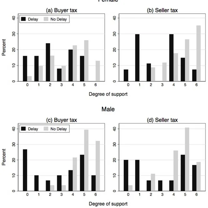
Figure 4 plots average support rates for the buyer and seller taxes. It shows that the delay of the tax benefit had a significant negative impact on the support rate for both taxes and for both genders. Among females, the delay effect decreased the support rate for the buyer tax by 25% and decreased the support rate for the seller tax by 31%. Among males, the delay effect was even stronger: the delay of the tax benefit decreased the support rate for the buyer tax by 46% and decreased the support rate for the seller tax by 31%. All these decreases were highly significant (Z-tests, p < 0.026). The distribution of degree of support shown in Figure 5 portrays a similar delay effect pattern. For males and females alike, attitudes towards both taxes shifted to negative when the tax benefit was delayed.
11
Figure 5: Distribution of degree of support in the first ballot and delay effect
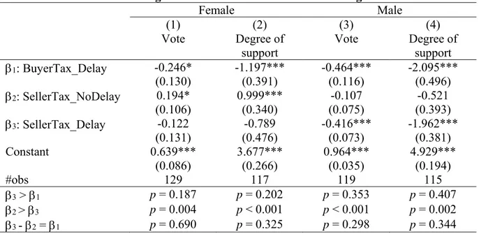
We also compared the negative delay effect between the buyer tax and the seller tax using a difference-in-difference regression analysis. Specifically, we ran a linear probability regression in which the probability of voting in favour of the tax was regressed on treatment dummies using BuyerTax_NoDelay as benchmark. Similarly, we ran an OLS regression in which the degree of support was the dependent variable. Table 2 shows the regression results separately by gender. The key difference-in-difference hypothesis tests of the delay effects between the different tax
12
frames are reported in the last row (3 - 2 = 1), which suggests that the delay effects did not differ between the buyer and seller taxes. Furthermore, the regression results confirm the significant evidence of the tax shifting bias under No Delay conditions for females but not for males (we could not reject the hypothesis 2 > 0 for males). We also confirmed the significant evidence of delay effects across tax frames and genders (we always rejected the hypotheses 1 < 0 and 2 > 3) and the lack of evidence of tax-shifting bias under Delay conditions for either gender (we could not reject the hypothesis 3 > 1).
Table 2: Voting behaviour in the first ballot for both genders
Female Male (1) Vote (2) Degree of support (3) Vote (4) Degree of support 1: BuyerTax_Delay -0.246* (0.130) -1.197*** (0.391) -0.464*** (0.116) -2.095*** (0.496) 2: SellerTax_NoDelay 0.194* (0.106) 0.999*** (0.340) -0.107 (0.075) -0.521 (0.393) 3: SellerTax_Delay -0.122 (0.131) -0.789 (0.476) -0.416*** (0.073) -1.962*** (0.381) Constant 0.639*** (0.086) 3.677*** (0.266) 0.964*** (0.035) 4.929*** (0.194) #obs 129 117 119 115 3 > 1 p = 0.187 p = 0.202 p = 0.353 p = 0.407 2 > 3 p = 0.004 p < 0.001 p < 0.001 p = 0.002 3 - 2 = 1 p = 0.690 p = 0.325 p = 0.298 p = 0.344
Note: Both are linear regressions with clustered standard errors at group/market level.
*, ** and *** indicate statistical significance at 10%, 5% and 1% level, respectively.
Overall, our results show that the negative effect of delay on the support rate was robust regardless of whether it was imposed on buyers or sellers. On the one hand, female voters were more willing to support the tax when it was imposed on sellers than on buyers, but their tax-shifting bias did not help promote tax support when the tax benefit was delayed. On the other hand, male voters were not subject to tax-shifting bias, and they were similarly biased against the tax when the benefit was delayed. Tiezzi and Xiao (2016) showed that learning helped voters become more supportive of the tax in the second ballot under No Delay conditions, although it had no impact when the benefit was delayed. We next examined whether this changed when the tax was imposed on sellers.
13
3.3 Learning
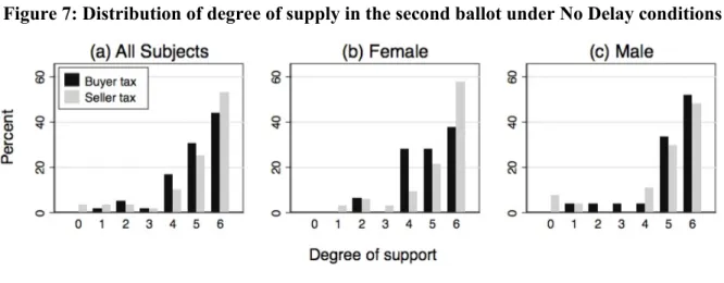
Figure 6 shows the average tax support rate and Figure 7 plots the distribution of degree of support in the second ballot under No Delay conditions. Here, in contrast to the first ballot, female voters did not show tax-shifting bias, but the tax support rate was consistently high at 90%, irrespective of tax frame or gender. The distributions of degree of support in the second ballot also suggest that most participants showed some degree of support for both the buyer and seller taxes (Figure 7). Our results (for females) are consistent with previous work on tax-shifting bias in experimental markets with externalities. For example, Sausgruber and Tyran (2011) found that inexperienced voters were prone to tax-shifting bias and that experience was an effective de-biasing mechanism.
Figure 6: Tax support rate in the second ballot under No Delay conditions
14
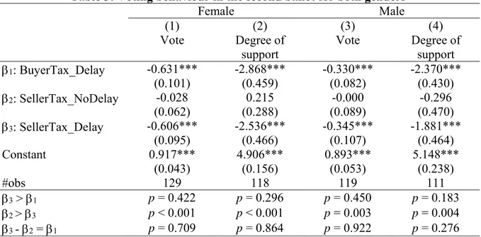
Next, we showed that although experience helped remove tax-shifting bias among female voters, it did not help reduce bias against the tax under Delay conditions. We re-estimated the models in Table 2 for the second ballot. Table 3 shows that the delay effect remained significant for both taxes (we rejected hypotheses 1 < 0 and 2 > 3, respectively). We also confirmed that tax-shifting bias was eliminated for females and remained nil for males (we could not reject the hypotheses 2 > 0 and 3 > 1). Finally, the delay effects in the second ballot did not differ across tax frames (we could not reject the hypothesis 3 - 2 = 1).
Table 3: Voting behaviour in the second ballot for both genders
Female Male (1) Vote (2) Degree of support (3) Vote (4) Degree of support 1: BuyerTax_Delay -0.631*** (0.101) -2.868*** (0.459) -0.330*** (0.082) -2.370*** (0.430) 2: SellerTax_NoDelay -0.028 (0.062) 0.215 (0.288) -0.000 (0.089) -0.296 (0.470) 3: SellerTax_Delay -0.606*** (0.095) -2.536*** (0.466) -0.345*** (0.107) -1.881*** (0.464) Constant 0.917*** (0.043) 4.906*** (0.156) 0.893*** (0.053) 5.148*** (0.238) #obs 129 118 119 111 3 > 1 p = 0.422 p = 0.296 p = 0.450 p = 0.183 2 > 3 p < 0.001 p < 0.001 p = 0.003 p = 0.004 3 - 2 = 1 p = 0.709 p = 0.864 p = 0.922 p = 0.276
Note: Both are linear regressions with clustered standard errors at group/market level. *, ** and *** indicate
statistical significance at 10%, 5% and 1% level, respectively. 4. CONCLUSION
We conducted a controlled laboratory experiment to investigate whether a previously observed delay effect on public support for Pigouvian taxation remained when the tax was levied on sellers. We found that although female buyers were subject to tax-shifting bias, it did not help mitigate the delay effect. Male buyers, on the other hand, did not show tax-shifting bias, but were similarly biased against the tax when its benefit was delayed. This finding provides converging evidence for the relevance of delayed benefit in determining support for the tax, as argued in Tiezzi and Xiao (2016).
15
Previous research on the LSE suggested that policy makers could increase public support for taxation by exploiting tax-shifting bias in the design of a new tax, e.g. a carbon tax on the seller side of the market rather than the consumer side (Gamage and Shankske 2011). Our findings show that such a design may have limited success when the tax aims to control externalities that have detrimental effects on social welfare over time. More research is needed to design and test mechanisms that can affect public attitudes to taxation in a dynamic setting.
16 REFERENCES
Blaufus, Kay, and Axel Möhlmann. 2014. “Security Returns and Tax Aversion Bias: Behavioral Responses to Tax Labels.” Journal of Behavioral Finance 15 (1): 56–69.
Borck, Rainald, Dirk Engelmann, Wieland Muller, and Hans-Theo Normann. 2002. “Tax Liability-Side Equivalence in Experimental Posted-Offer Markets.” Southern Economic
Journal 68 (3): 672.
Cherry, Todd L., Steffen Kallbekken, and Stephan Kroll. 2017. “Accepting Market Failure: Cultural Worldviews and the Opposition to Corrective Environmental Policies.” Journal of
Environmental Economics and Management 85: 193–204.
Collier, Paul, and Anthony J. Venables. 2014. “Closing Coal: Economic and Moral Incentives.”
Oxford Review of Economic Policy 30 (3): 492–512.
Cox, James C, Mark Rider, and Astha Sen. 2017. “Tax Incidence: Do Institutions Matter? An Experimental Study.” Public Finance Review, April, forthcoming.
Dresner, Simon, Louise Dunne, Peter Clinch, and Christiane Beuermann. 2006. “Social and Political Responses to Ecological Tax Reform in Europe: An Introduction to the Special Issue.” Energy Policy 34 (8): 895–904.
Fischbacher, Urs. 2007. “Z-Tree: Zurich Toolbox for Ready-Made Economic Experiments.”
Experimental Economics 10 (2): 171–78.
Gamage, David, and Darien Shankske. 2011. “Three Essays on Tax Salience: Market Salience and Political Salience.” Tax Law Review 65: 19–98.
Kachelmeier, Steven J., StephenT. Limberg, and Michael S. Schadewald. 1994. “Experimental Evidence of Market Reactions to New Consumption Taxes.” Contemporary Accounting
Research 10 (2): 505–45.
Kallbekken, Steffen, Stephan Kroll, and Todd L. Cherry. 2010. “Pigouvian Tax Aversion And Inequity Aversion In The Lab.” Economics Bulletin 30 (3): 1914–21.
———. 2011. “Do You Not like Pigou, or Do You Not Understand Him? Tax Aversion and Revenue Recycling in the Lab.” Journal of Environmental Economics and Management 62 (1): 53–64.
Kerschbamer, Rudolf, and Georg Kirchsteiger. 2000. “Theoretically Robust but Empirically Invalid? An Experimental Investigation into Tax Equivalence.” Economic Theory 16: 719– 34.
17
Lazarus, Michael, Peter Erickson, Kevin Tempest, and Michael Lazarus. 2015. “Supply-Side Climate Policy: The Road Less Taken.” Stockholm Environmental Institute Working Paper 2015-13.
Menges, Roland, and Stefan Traub. 2008. “Energy Taxation and Renewable Energy: Testing for Incentives, Framing Effects and Perceptions of Justice in Experimental Settings.” In 2008
5th International Conference on the European Electricity Market, 1–8. IEEE.
Metcalf, Gilbert E, and David Weisbach. 2009. “The Design of a Carbon Tax.” Harvard
Environmental Law Review 33 (2): 499–556.
Morone, Andrea, Francesco Nemore, and Simone Nuzzo. 2016. “Experimental Evidence on Tax Salience and Tax Incidence.” Kiel Working Paper No. 2063.
Riedl, Arno, and Jean-Robert Tyran. 2005. “Tax Liability Side Equivalence in Gift-Exchange Labor Markets.” Journal of Public Economics 89 (11–12): 2369–82.
Rivlin, Alice M. 1989. “The Continuing Search for a Popular Tax.” American Economic Review 79 (2): 113–17.
Ruffle, Bradley J. 2005. “Tax and Subsidy Incidence Equivalence Theories: Experimental Evidence from Competitive Markets.” Journal of Public Economics 89 (8): 1519–42. Sausgruber, Rupert, and Jean-Robert Tyran. 2011. “Are We Taxing Ourselves?” Journal of
Public Economics 95 (1–2): 164–76.
Sausgruber, Rupert, and Jean Robert Tyran. 2005. “Testing the Mill Hypothesis of Fiscal Illusion.” Public Choice 122 (1–2): 39–68.
Schenk, Dh. 2011. “Exploiting the Salience Bias in Designing Taxes.” Yale Journal on
Regulation 28 (2): 253–311.
Tiezzi, Silvia, and Erte Xiao. 2016. “Time Delay, Complexity and Support for Taxation.”
Journal of Environmental Economics and Management 77 (May): 117–41.
Weber, Matthias, and Arthur Schram. 2017. “The Non-Equivalence of Labour Market Taxes: A Real-Effort Experiment.” Economic Journal 127 (604): 2187–2215.
18
Appendix A Additional Figure
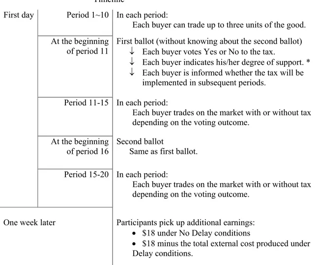
Figure A1: Timeline of the experiment Timeline
First day Period 1~10 In each period:
Each buyer can trade up to three units of the good. At the beginning
of period 11
First ballot (without knowing about the second ballot) Each buyer votes Yes or No to the tax.
Each buyer indicates his/her degree of support. * Each buyer is informed whether the tax will be
implemented in subsequent periods. Period 11-15 In each period:
Each buyer trades on the market with or without tax depending on the voting outcome.
At the beginning of period 16
Second ballot
Same as first ballot. Period 15-20 In each period:
Each buyer trades on the market with or without tax depending on the voting outcome.
One week later Participants pick up additional earnings:
$18 under No Delay conditions
$18 minus the total external cost produced under Delay conditions.
* The timeline is identical to that of Tiezzi and Xiao (2016) except that we investigated degree of support.
19
Appendix B Experimental Instructions
B.1 Instructions regarding the auction
(All treatments)
General
Thank you for coming! You’ve earned $5 for participating, and the instructions explain how you can make decisions and earn more money which will be paid to you in cash.
This is an experiment in the economics of market decision making. In this experiment we are going to simulate a market in which each participant will be a buyer in a sequence of trading periods. There should be no talking at any time during this experiment. If you have a question, please raise your hand, and an experimenter will assist you.
During the experiment your earnings will be calculated in experimental points. Experimental points will be converted in Dollars at the following exchange rate:
200 experimental points = 1$
At the end of today’s experiment you will receive, in cash, the earnings you make today. In addition, you will receive a payment certificate to pick up your $5 participation bonus and an additional cash payment of $18 the same day next week.
For example, if today is Monday, you will receive the $5 participation bonus and the additional $18 cash payment next Monday. To pick up these amounts, you need to come back to the same lab the same day next week (if you cannot make it at the time indicated on your payment certificate please send an email to [the experimenter’s email address] to schedule another time on the same day or you can send someone else to pick up your cash payment on the same day). You do not need to participate in any decision task next week to receive the additional $18 payment.
(Delay only)
However, as we describe below, you may lose some of this $18 depending on the decisions you and the other three buyers in your market make today. The final amount of the additional cash payment you pick up next week will therefore depend on the decisions you and the other three buyers in your market make in today’s experiment.
(All treatments)
In today’s experiment, you will first participate in two practice trading periods followed by a number of paid trading periods. In the practice trading periods you do not earn money, but you should take these periods seriously since you will gain valuable experience for the paid trading periods.
20 Specific instructions to buyers
In this experiment each participant is a buyer. Each buyer is randomly assigned to a group of 4 buyers – a market – and remains in the same market with the same buyers throughout the experiment. What is happening in other markets is irrelevant for your own market and hence for your own earnings. During each trading period each buyer can buy units (up to 3 units) of a hypothetical consumption good from an automated (computerized) seller.
Resale value of a unit. At the beginning of each trading period, you will be given three separate
resale values for each of the three units of the good you can purchase. These are your privately known resale values. You can think of the resale value of a unit as the potential earnings you can make out of that unit. Your resale values will remain the same in each period during the experiment.
Bid. As a buyer, you can submit a “bid” to buy a unit from the seller during a trading period. A
“bid” is the amount you are willing to pay for that unit of the good. You must submit one “bid” for each of the three units. (If you do not want to purchase a unit, you may simply submit a bid “0”.) Your bids have to follow the following two rules: 1) “Trade at no loss”: your bid for each unit cannot be above your resale value for that unit; 2) Your bid for the third (second) unit cannot be above your bid for the second (first) unit.
How the market works
At the beginning of each trading period each buyer submits bids for each unit offered in the market. At the end of each trading period, all submitted bids are collected and ranked from high to low. If two or more bids are equal, ranks will be randomly assigned by the computer.
1. How the Market Price is determined
The automated seller has a production cost unknown to all buyers. The production cost does not change during the experiment. The seller never trades at a loss, therefore it will not accept bids below its production cost. The seller will accept, among all bids from all buyers in the market, the lowest bid above or equal to the production cost. This will be the per-unit Market Price. Bids that are below the production cost will be rejected and buyers who have submitted those bids won’t buy any units (i.e. buyers will neither pay for those units they placed a bid nor gain any resale value from those units).
The market price can be different in each period because it depends on the bids that are submitted in each period.
2. How the Market Quantity is determined
Buyers will purchase a unit when their bid is greater than or equal to the market price. The Market Quantity is the total number of units purchased by the 4 buyers in one market in one period at the market price.
21
Example: Suppose, in one market and in one trading period, the automated seller’s production cost is 70. And suppose the automated seller collects the following bids from the 4 buyers.
Buyer 1 Buyer 2 Buyer 3 Buyer 4
Bid Unit 1 135 135 140 145
Bid Unit 2 85 90 94 85
Bid Unit 3 80 0 80 40
The bids are ranked from high to low as follows: 145, 140, 135, 135, 94, 90, 85, 85, 80, 80, 40, 0. In this case, the Market Price is 80 (the lowest bid above the production cost of 70). All 10, and only the 10 units for which the bids were equal or above the market price of 80 will be purchased by the buyers who submitted the corresponding bids. These 10 sold units are bolded in the table. Each of these 10 units will be exchanged at 80. The market quantity in this case is 10. The number of sold units is determined by the number of submitted bids above or equal to the market price. Units for which the submitted bids are below the market price will not be sold.
Please note: The information on values and production costs of a unit is private. Buyers do not know the bids of other buyers, nor do they know the per-unit production cost for the seller.
(No Delay only)
3. Additional Costs from Trading
Each unit traded in the market (i.e. each unit sold) causes an additional cost of 60 points that will be equally split by the 4 buyers in the market. This means that each of the 4 buyers in the market has to pay an additional cost of 60/4=15 points. Note that you will bear a share of the additional costs even if you do not buy any units yourself.
Using the example above where the market quantity is 10 units, in this case, each buyer incurs an additional cost of (60/4)*10=150 points=$0.75.
4. How your earnings today in each trading period are calculated
Your Final earnings in one trading period = Gross earnings in the trading period - Additional Costs per person in the trading period, where
Gross earnings in the trading period= (Resale value - Market price) of each unit purchased In the example above Buyer 4 buys two units. Her resale value for Unit 1 is 200, her resale value for Unit 2 is 140 and her resale value for Unit 3 is 100. The market price is 80. Her Gross earnings
22
in this period = 200 (resale value of Unit 1) + 140 (resale value of Unit 2) – 2*80 (market price) = 340 – 160 = 180
Since the market quantity is 10, the additional costs per person are (60/4)*10 = 150. Her Final earnings in this period =180 (Gross earnings) – 150 (Additional costs per person) = 30.
As you can see, in this case, even though Buyer 4’s resale value for Unit 3 is 100, which is higher than the market price 80, Buyer 4 did not purchase the unit because her bid for Unit 3 (40) is lower than the market price (80).
Your total Final earnings for today are the sum of your Final earnings in each trading period over all the paid trading periods.
5. How your earnings next week are calculated
Each participant will receive $18 next week. You do not need to participate in any decision task next week to receive the cash payment for the next week. You just need to pick it up in the lab on the same day next week.
(Delay only)
3. Additional Costs from Trading
Each unit traded in the market (i.e. each unit sold) causes an additional cost of 60 points that will be equally split by the 4 buyers in the market. This means that each of the 4 buyers in the market has to pay an additional cost of 60/4=15 points. Note that you will bear a share of the additional costs even if you do not buy any units yourself.
Using the example above where the market quantity is 10 units, in this case, each buyer incurs an additional cost of (60/4)*10=150 points=$0.75.
These additional costs will not affect your earnings today but will be deducted from the $18 cash payment you will receive next week.
4. How your earnings today in each trading period are calculated
Your Final earnings in one trading period = (Resale value - Market price) of each unit purchased In the example above Buyer 4 buys two units. Her resale value for Unit 1 is 200, her resale value for Unit 2 is 140 and her resale value for Unit 3 is 100. The market price is 80. Her Final earnings in this period are = 200 (resale value of Unit 1) + 140 (resale value of Unit 2) – 2*80 (market price) = 340 – 160 = 180
23
As you can see, in this case, even though Buyer 4’s resale value for Unit 3 is 100, which is higher than the market price 80, Buyer 4 did not purchase the unit because her bid for Unit 3 (40) is lower than the market price (80).
Your total Final earnings for today are the sum of your Final earnings in each trading period over all the paid trading periods.
5. How your earnings next week are calculated
Each participant will receive $18 next week. However, the final amount of the cash payment you will pick up next week will depend on the decisions you and the other 3 buyers in your market make today.
In the example above, since the market quantity is 10, the additional costs per person are (60/4)*10 = 150 points. This additional cost will be deducted from Buyer 4’s cash payment for the next week. So, the final payment each buyer will receive next week = $18 - the Sum of the Additional Cost per person in each period today.
You do not need to participate in any decision task next week to receive the cash payment for the next week. You just need to pick it up in the lab on the same day next week.
24
B.2 Voting Instructions (Seller tax treatments)
You and the other three participants in your market will now vote whether to introduce a tax of 60 points on the seller on each sold unit of the good. If at least two out of four buyers in each market vote “Yes”, the tax is accepted and the following changes are implemented for the following trading periods: 1) the seller pays a tax of 60 points for each unit she sells; 2) at the end of each period, each buyer will receive an equal share (one-fourth) of the total tax revenues collected from all units sold by the seller in your market. All the other rules described in the instructions for the first 10 trading periods remain the same. In particular, seller’s production cost and each buyer’s resale value of each unit remain the same as the previous 10 periods.
Example
Suppose the tax of 60 points per unit is accepted as the outcome of the voting in your market. To illustrate how this would affect the outcome of the market and your earnings we use the same example from the instructions for the first 10 trading periods. In that example, when the automated seller sells one unit of the good, her production cost of this unit is 70 points but now she will also have to pay the tax of 60 points. The total cost of each sold unit for the seller will now be 70 +60 =130. Consider Buyer 4. Buyer 4’s resale value for Unit 1 is 200, her resale value for Unit 2 is 140 and her resale value for Unit 3 is 100.
Consider again the example in which the seller collects the following bids from the 4 buyers.
Buyer 1 Buyer 2 Buyer 3 Buyer 4
Bid Unit 1 135 135 140 145
Bid Unit 2 85 90 94 85
Bid Unit 3 80 0 80 0
(No Delay only)
To illustrate how a buyer’s earnings today are calculated, again let’s use the example of Buyer 4. Since the Market price is 135, Buyer 4 buys 1 unit. Buyer 4’s gross earnings in this period = 200 (resale value of unit 1) – 135 (market price) = 65.
Since the Market quantity is now 4, in this period the Additional costs per person are (60/4)*4 = 60 points. Since 4 units are sold, the total tax revenues in this period are 4*60=240. One fourth of the total tax revenues, 240/4=60 points, will be returned to Buyer 4.
25
Buyer 4’s Final earnings in this period = 65 (Gross earnings) – 60 (Additional costs per person) + 60 (returned tax revenues) = 65.
Suppose the tax proposal is rejected.
Trading will continue as before the vote and no changes will apply. Thus, in the above example, the seller will only accept bids above or equal to the production cost 70. The Market price is therefore 80. Buyer 4 buys two units. Her gross earnings for that period are 180.
Since the Market quantity is 10, in this period the additional costs per person are (60/4)*10=150 points. Her final earnings for that period are 180-150=30. All final earnings in the following periods will be calculated as illustrated above.
(Delay only)
To illustrate how a buyer’s earnings today are calculated, again let’s use the example of Buyer 4. Since the Market price is 135, Buyer 4 buys 1 unit. Since 4 units are sold, the total tax revenues in this period are 4*60=240. One fourth of the total tax revenues, 240/4=60 points, will be returned to Buyer 4.
Buyer 4’s Final earnings in this period = 200 (resale value of unit 1) - 135 (market price) + 60 (returned tax revenues) = 125.
Since the Market quantity is now 4, in this period the Additional costs per person are (60/4)*4 = 60 points. These additional costs will not affect Buyer 4’s earnings today but will be deducted from the $18 cash payment Buyer 4 will receive next week.
So, the final cash payment each buyer will receive next week = $18 - the sum of the Additional Cost per person in each period.
Suppose the tax proposal is rejected.
Trading will continue as before the vote and no changes will apply. Thus, in the above example, the seller will only accept bids above or equal to the production cost 70. The Market price is therefore 80. Buyer 4 buys two units. Her final earnings for that period are 180.
Since the Market quantity is 10, in this period the additional costs per person are (60/4)*10 = 150 points. Again, these additional costs will be deducted from the cash payment Buyer 4 will receive next week. All final earnings in the following periods will be calculated as illustrated above.
(Both treatments)
You will be informed about the outcome of the vote in your group on the screen before the trading continues. Nobody, however, will be informed about individual votes of other participants. In the
26
ballot, all participants simultaneously vote Yes or No for the introduction of the tax. Abstentions or neutral votes are not possible. Voting is anonymous.
Before proceeding to the vote you will be asked to do an exercise to make sure you understand the instructions.
If you now have questions, please, raise your hand and wait until an experimenter will come by to answer your questions individually.