Modelling the Hydrologic Behavior of the
Upper Tiber River Basin under Climate
Change Scenarios
Fiseha Behulu Muluneh
Roma, April 2013
ROMA TRE
PhD Research Thesis
PhD SCHOOL OF ENGINEERING
CIVIL ENGINEERING SECTION
XXV CYCLE
Modelling the Hydrologic Behavior of the Upper Tiber River
Basin under Climate Change Scenarios
Candidate:
__________________
Fiseha
Behulu
Muluneh
Major Supervisor (s):
__________________
prof. Aldo Fiori
Co - Supervisor:
Dr. Assefa M. Melese
__________________
PhDCoordinator:
Collana delle tesi di Dottorato di Ricerca In Scienze dell’Ingegneria Civile
Università degli Studi Roma Tre Tesi n° 38
Dedicated to:
my mother, Aberash Belayneh; the departed soul of my father Behulu Muluneh; my brothers and sisters; my wife Bizunesh Wodajo; and my son Yeabsira Fiseha.
Abstract
Quantification of the various components of hydrological processes in a watershed remains a challenging topic as the hydrological system is altered by internal and external drivers. This study investigates hydrological behavior of the Upper Tiber River Basin (UTRB) in central Italy under climate change scenarios. It addresses the response of the watershed by evaluating the relative changes in magnitudes of various hydrological processes using downscaled climate data in a watershed model. The observed data from regional concerned offices of the basin and the readily available global and regional climate model data were collected for analysis.
First, the reliability of the precipitation and temperature data through two statistical downscaling methods are evaluated. The Statistical Downscaling Model (SDSM) and the Long Ashton Research Station Weather Generator (LARSWG) are used to downscale the HadCM3 GCM predictions of the A2 and B2 scenarios for the Chiascio sub-basin in the UTRB. The results show that the downscaling methods used have different performance to reproduce the precipitation patter but they agree on both minimum and maximum temperature. However it is difficult to choose which method is of downscaling as both have their own limitations and associated uncertainties
Second, a physically-based watershed simulation model called Soil Water Assessment Tool (SWAT) is used to understand the hydrologic behavior of the basin. The model is successfully calibrated for the period of 1963-1970 and validated for the period of 1971-1978 using observed weather and flow data. A total of eighteen hydrologic parameters are evaluated and the model showed high relative sensitivity to groundwater flow driven parameters than the surface
flow driven parameters. The objective function for model evaluation statistics showed coefficient of determination (R2) from 0.68 to 0.81 and Nash Sutcliffe Efficiency (ENS) between 0.51 and 0.8 for the validation period. Based on the
calibrated parameters the model is proved to be capable of predicting impact of climate changes in water resources planning and management.
Third, the calibrated watershed model is used to evaluate the response of the basin under different climate change scenarios. Bias correction to three regional climate model (RCM) from the PRUDENCE including RegCM, RCAO, and PROMES outputs are applied. The current (1961-1990) and future (2071-2100) time periods were considered for the analysis. The result indicated that there will be significant decrease in the hydrologic components and water yields of the basin which resembles some previous findings in the basin. The result of the present study is different from the others in that most of them used indices based on observation. However, future work on the uncertainty issues related to projected climate variables is highly recommended. Despite some common limitations, this study is relevant to assist the development of climate change adaptation in the study.
Acknowledgements
First and for the most praise be unto the Almighty God Who gave me all the courage and power throughout my achievements. Next, I would like to forward my heartfelt thanks to those who helped me at different stages of my present PhD work.
I would like to extend my utmost words of thanks to my first supervisor Prof. Aldo Fiori for his great guidance, constructive supports and critical comments throughout my PhD research work. Aldo taught me how to react positively to comments in research and publication and he made me free to work independently on my research activity. He was so understanding person, and it is not an exaggeration to say ‘working with Aldo is like working with a real and caring father’
The contribution of my co-supervisor, Dr. Assefa Mekonnen Melese on the current PhD work is also have got high impact. He hosted me at Florida International University (FIU), USA in Hydrology and Geo-Spatial laboratory for one year where I have got deep insights to hydrological modeling. Every communications I made with Assefa were so fruitful and I hope that will remain intact in our future collaborations.
I am thankful for the Italian government who has granted me a three year scholarship fund to cover my expenses during my stay in Italy and during my study abroad in USA. I am also grateful to Dr. Elena Volpi from Civil Engineering Department of Roma Tre, who has introduced me to the basics of MATLAB coding and commented most of my works. I am also thankful to Dr. Emanuele Romano from National research center of Rome, for his provision of essential data set for my research and his contribution to some of the published works. My sincere thanks also goes to Dr. Shimelis Gebriye Setegn of Earth and Environment department at FIU for his guidance and encouragement to write scientifically publishable papers.
I am highly delighted to express acknowledgements to Pietro, Claudia, Antonio, Elisabetha, Federico, Francesca and Alesandro Romano for the hospitalities they have shown me during my stay at Roma Tre. They all were too friendly and helpful regardless of the language barrier. I also acknowledge the Ethiopian students and friends, Melkamu Alebachew (Melke) of Roma Tre and Ademe Zeyede of Tor-Vergata, whom we shared sweet time in the ancient city of Rome for the last three years during my PhD study. Melke and Ademe- there was no home sick due to both of you. Among other country mates I had had the acquaintance in Italy, the contribution of Tsehay Simeneh, Tewabech Woldegeorgis and Wondwosen Demelash was so grateful and I say let God bless them all.
Most importantly, had it been possible to do so, at every step of my success, I would have written a separate book of acknowledgements about my mother’s passion and effort to bring me up to this level. However, at this step, I can only say let God gives her an endless health. “Emaye” once again, I say “your blessings are the slogan of my success”.
Finally, I appreciate and thank my wife Bizunesh Wodajo Bulti (Emuye) who has taken all the burden during my absence for study leave. Our new son Yeabsera Fiseha Behulu will benefit a lot from the love we have to each other!
Table of contents
List of Figures ... xi
List of Tables... xiii
Acronyms and Abbreviations ... xiv
1. Introduction ... 1
1.1. General background ... 1
1.2. Objective of the research ... 4
1.3. Overall framework of the research ... 6
1.4. Structure of the thesis... 8
2. Climate Change and Water Resources :A Short Review ... 10
2.1. General ... 10
2.2. Climate Models in Water Resources Studies ... 14
2.2.1.GCM for Water Resources Studies ... 14
2.2.2.RCM for Water resources Studies ... 17
2.2.3.Scale issues in water resources modelling and climate change impact studies ... 20
2.3. Known Methodologies for Climate Change Impact Assessment 22 2.3.1 The direct use of GCM outputs in hydrological models .. 22
2.3.2.Coupling GCMs and Macro-Scale Hydrologic Models ... 24
2.3.3.Downscaling GCM to Force Hydrological Models ... 26
2.3.4. Using hypothetical scenarios in Hydrological Models .... 33
2.4. Review of Climate Change Impact on Water Resources ... 35
2.4.1.Impact Studies on Surface Water Resources... 37
2.4.2.Impact Studies on Groundwater Resources ... 41
2.5. Climate Change in Italy ... 44
3. Study Area Description ... 52
3.1. Location and General Characteristics ... 52
3.2. Topography, Geology, Land use and Soils ... 54
3.3.1.Rainfall data ... 64
3.3.2.Temperature Data ... 71
3.3.3.River Flow Data ... 75
3.4. Summary ... 77
4. Downscaling Climate Model Outputs from Single GCM ... 81
4.1. Background ... 82
4.2. Study Area and Data Used ... 83
4.2.1.Study Area ... 83
4.2.2.The Datasets ... 85
4.3. Downscaling Daily Precipitation and Temperature Time Series 88 4.3.1.Downscaling Model Description and Setup ... 88
4.3.2.Calibration and Validation of SDSM ... 90
4.3.3.Calibration and Validation of LARS-WG ... 96
4.4. Results and Discussions ... 98
4.4.1.Downscaling with SDSM ... 98
4.4.2.Downscaling with LARS-WG ... 101
4.5. Final Remarks ... 105
4.6. Conclusion ... 107
5. Watershed Modelling ... 110
5.1. General background ... 110
5.1.1.Overview of Watershed Model Classification ... 111
5.1.2.Model Selection Criteria ... 114
5.2. The Soil and Water Assessment Tool (SWAT) ... 115
5.2.1.Surface Runoff in SWAT ... 118
5.2.2.. Evapotranspiration Estimation in SWAT ... 121
5.2.2.Soil Water Estimation in SWAT ... 121
5.2.3.Groundwater in SWAT Model ... 122
5.3. Study Area and Model Setup ... 126
5.3.1.Study Area and Data sources ... 126
5.3.2.Models Setup ... 129
5.3.3.Sensitivity Analysis and Calibration ... 132
5.4. Results and Discussions ... 136
5.4.1.Results of Sensitivity analysis and model calibration .... 136
5.4.2.Validation and Performance Evaluation of SWAT ... 143
5.4.3.Hydrological Water Balance of UTRB based on SWAT ... 146
5.5. Conclusions ... 152
6. Impact of Climate change on the Hydrology of Upper Tiber River Basin Using Bias Corrected Regional Climate Model ... 155
6.1. Introduction ... 156
6.2. Materials and Methods ... 158
6.2.1..Climate and Hydrology data ... 159
6.2.2..Description of the Hydrological Model ... 160
6.3. Regional Climate Model Outputs ... 163
6.4. Interfacing between RCM and Hydrological Model ... 166
6.5. Results and Discussion ... 168
6.5.1.Calibration and Validation of the SWAT Model ... 168
6.5.2.Bias Correction results of Precipitation and temperature Variables ... 169
6.5.3.Hydrological response to climate change ... 172
6.5.4.Uncertainty issues and further considerations ... 179
6.6. Conclusion ... 181
7. Conclusions and Recommendations ... 183
7.1. Conclusion ... 183
7.2. Recommendations ... 185
7.3. Future Research ... 186
References ... 187
List of Figures
1.1. General flow of the research 7
2.1. Progress in application of downscaling for hydrological impact
studies (last accessed Dec 28/2010) 13
2.2. Schematic representation of the methods for assessing water
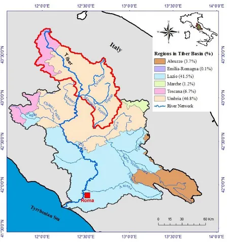
resources under changing climate (Source:- Xu and Singh, 2004). 23 3.1. The Tiber River Basin and the regions it crosses in central Italy. The
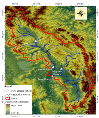
red boundary shows the area used for hydrological simulation and
analysis. 53
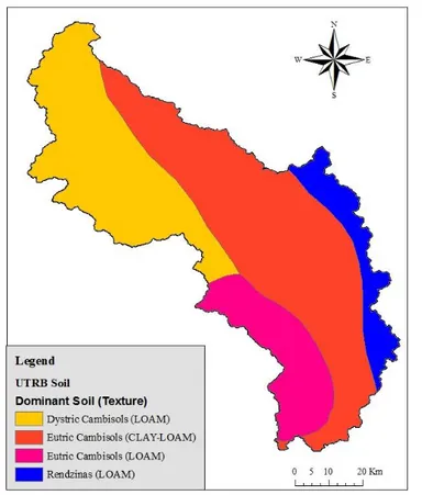
3.2. Digital Elevation Model (DEM) and River Networks in the UTRB 56 3.3. Dominant Soil classes in the Upper Tiber River Basin 57
3.4. Land uses in the Upper Tiber River Basin 59
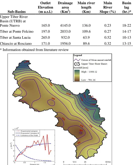
3.5. Mean annual rainfall variation in the Upper Tiber Basin (The Variogram model used in the Ordinary Kriking shown in the lower
left corner). 63
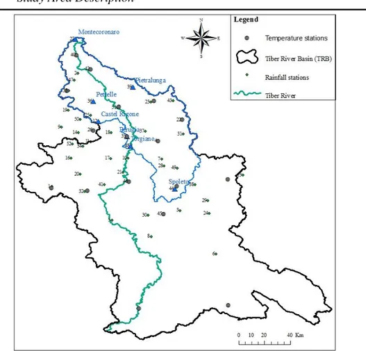
3.6. Mean annual precipitation anomaly for the study area (1961-1990) 65 3.7. Location of rainfall and temperature gauging stations in TRB (the
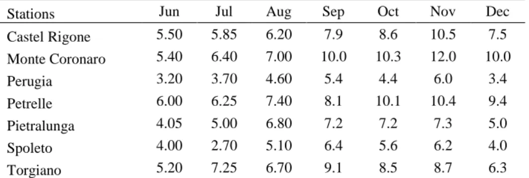
numbered labels show the corresponding station name in Table 32). 67 3.8. Box plots of the daily rainfall at seven selected stations in the UTRB. 70 3.9. Inter-annual variability of daily maximum temperature at selected
stations in the UTRB (January 1, 1961- December 31, 1990). The
95% confidence intervals of the mean values are also shown. 72 3.10 Inter-annual variability of daily minimum temperature at selected
stations in the UTRB (January 1, 1961- December 31, 1990). The
95% confidence intervals of the mean values are also shown. 73 3.11 Variation of daily maximum temperature (upper panel) and daily
minimum temperature (lower panel) with elevation for the dry months
(JJA) in the TRB. 74
3.12 Flow gauging stations and their corresponding frequency of flow. 76 3.13 Daily maximum and minimum flows in the dry and wet seasons at
Ponte Nuovo gauging station. 77
4.1. Location map of the Upper-Tiber River basin and the gauging
stations 84
4.2. Validation results of SDSM-based downscaling for Precipitation
4.3. Validation results SDSM-based downscaling for Tmax and Tmin
(1981-1990) 95
4.4. Comparison of observed and generated data with LARS-WG for
precipitation. 97
4.5. Trends of precipitation at Assisi station under A2 and B2 Scenario
downscaled with SDSM. 100
4.6. Trends of Temperature (min and max) at Assisi station under A2 and
B2 Scenario downscaled with SDSM. 101
4.7. Downscaled results of Precipitation using LARS-WG. 103 4.8. Downscaled results of Temperature (Tmin and Tmax) using
LARS-WG 104
5.1. Schematic representation of the hydrologic cycle in SWAT (Source:
Neitsch et al., 2009) 117
5.2. Conceptual representation of hydrologic processes in SWAT (after:
Luo et al., 2012) 120
5.3. Location, DEM, and major sub-basins of the UTRB used for SWAT
simulation 127
5.4. Auto-calibration results for monthly flow at Ponte Nuovo (1963-1970) 138 5.5. Manual calibration results for monthly flow at Ponte Nuovo
(1963-1970) 139
5.6. Flow duration curves for Ponte Nuovo on daily data. 140 5.7. Average base flow contribution at Ponte Nuovo outlet during the
calibration period (1963-1970) 142
5.8. Simulated versus observed flow during validation period 144 5.9. Observed and simulated base flow contribution from the three
sub-basins during the validation period (1991-1995) 145
6.1. Location and DEM of the Upper Tiber River Basin 160
6.2. Calibration results for monthly flow at Ponte Nuovo (1963-1970) 169 6.3. Simulated vs observed flow during validation periods at Ponte Nuovo 169 6.4. Average annual change in river flow at Ponte Nuovo under A2 and
B2 Scenarios 175
6.5. Monthly flow duration curves (FDC) for flow at the sub-basin outlet (Ponte Nuovo). The left panels show the FDC for the A2 scenario and
the right panels show the FDC for B2 scenario. 176
6.6. Change in baseflow contribution in the UTRB under A2 and B2
Scenarios 177
6.7. The spatial distribution on the relative changes in groundwater
List of Tables
2.1. Comparative summary of the relative advantages and disadvantages of dynamical and statistical downscaling method (adapted from Fowler,
2007) 32
3.1. Summary of major physiographic characteristics of the UTRB 63 3.2. Selected rainfall stations in the Tiber River Basin (TRB). 66 3.3. The median values of the daily rainfall of the wet (SON) and dry (JJA)
months at seven selected stations in the upper Tiber River Basin
(UTRB). 69
3.4. Selected daily temperature (Tmin and Tmax) observation station in the
TRB 71
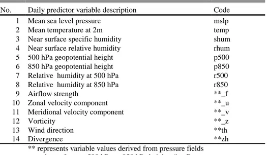
4.1. Summary of selected meteorological stations 86 4.2. Lists of large scale predictor variables from NECP and HadCM3 87 4.3. Summary of selected predictor variables with their respective
predictands 92
4.4. Performance of SDSM during the calibration and validation periods 96 5.1. Land use and land cover classes of the sub-basin 129 5.2. Selected hydrologic parameters included in SWAT sensitivity analysis
for the Upper Tiber River Watershed (Central Italy) 141 5.3. Performance of the model during the validation period 145 5.4. Annual water balance components at Ponte Nuovo outlet (all values are
in mm of water) 147
5.5. Average Annual water balance components at selected sub-basins
(1991-1995) 149
5.6. Average annual water balance components for the entire watershed (all
values are in mm of water) 149
5.7. Dry and wet years during the model calibration and validation at
different stations 150
5.8. Summary of water balance components for dry and wet years 151 6.1. Selected Regional Climate Model for hydrological impact assessment in
the Upper Tibe River Basin 164
6.2. Bias correction factors used to modify the simulated climate variables
for station at Assisi 171
6.3. Seasonal changes in precipitation (in %) and temperature (o C ) at
Assisi station 172
6.4. Comparison of mean annual water balance for the control and scenario
periods 174
Acronyms and Abbreviations
FAO Food and Agriculture Organization of the United Nations
a. m.s.l above mean sea level
CMIP3 Climate Model Intercomparison Project (third)
CORDEX Coordinated Regional Climate Downscaling Experiment
DEM Digital Elevation Model
FAR First Assessment Report of the IPCC
GCM Global Climate Model
GHGs Greenhouse Gases
GIS Geographic Information Systems
HadCM3 Hadley Centre for Climate Prediction and Research Coupled Model, version 3
HC The Hadley Centre
IPCC Intergovernmental Panel on Climate Change IRPI Istituto di Ricerca per la Protezione Idrogeologica
ITCP International Center for Theoretical Physics
LH-OAT Latin Hypercube sampling-One-Factor-At-a-Time
PRUDENCE Prediction of Regional scenarios and Uncertainties for Defining
EuropeaN Climate change risks and Effects
RCM Regional Climate Model
SMHI Swedish Meteorological and Hydrological Institute
SWAT Soil and Water Assessment Tool
TRB Tiber River Basin
UCM Universidad Complutense de Madrid
Chapter 1
This chapter is an overall preface to the research undertaken in this doctoral thesis. It provides a general background to the research with some issues related to climate change on water resources. The water resources problem in the Italian context with the motivation of the research was also provided un this background section. The objectives of the study are presented in section 1.2. Section 1.3, provides the overall framework of the research and finally, the structure of the present thesis is presented in section 1.4.
1. Introduction
1.1. General background
One of the challenge in water resources planning and management is to estimate future availability of water and to develop management strategies in the face of climate change. It is expected that global climate change will have a strong impact on water resources in many regions of the world (Bates et al., 2008). One of the most important impacts of future climatic changes on society will be the changes in regional water availability (Xu and Singh, 2004). In view of sustainable development, man has always remained very conscious of the requirements of water towards meeting the mandatory needs for food production, public health, energy needs, industrial development and production and other important
aspects of quality of life. Due to ever increasing demands for water in the recent times following the population growth and variations in the hydrological inputs, the problem of water management (i.e. the control of water in quantity and quality) as it passes through natural hydrological cycle with attention to maximizing economic, social and environmental goals, has become crucial. In water management planning, the basic complexity arises from conflicts among different objectives and various beneficiary groups of the society and their organizational structure. Thus planning for water resources must take into account the integration of these different objectives and interests for effective implementation.
As part of water resources planning objectives and potential assessment, small scale studies at watershed level now a days are getting due attention. In a watershed, numerous internal and external drivers act on the natural ecosystem regardless of their geographic locations. These effects of the drivers on the system understanding create a twofold problem. On one hand, the quantification of the hydrological processes (precipitation, evaporation, recharge, runoff, etc.) and storages taking place within the system is a scientific challenge. On the other hand, quantification of the drivers such as land cover change due to human interaction with the natural environment and real determination of climate change impact on the hydrologic processes is difficult. Also, studies revealed that over next few years an increasing population and increasing use of water will put high pressure on global water resources (Arnell, 1999). The aggregate impacts of both the internal and external drivers determine the amount and quality of water available in long run.
The development of hydrologic and watershed models has been the direct outcome of the need to integrate our knowledge on existing theories on real world flow behaviour with all physical and measured data. However, large-scale and complex environmental systems such as the global hydrological cycle or basin pollutant loading cannot be investigated directly through experimentation, but instead must be generalized into their component processes through modelling (Praskievicz and Chang, 2009). The key factor in model development has been and still is the on-going breakthrough in computation technologies particularly the introduction of the digital computer that is capable to store, manipulate data and to execute complex calculations beyond the physical ability of man, yet within his mental capacity.
The hydrologic cycle plays a key role in the energy balance of the earth’s surface-atmosphere system. The world’s water resources are impacted by global warming in complex manner associated with the changes in storage and fluxes in the general water balance equation of the hydrologic cycle. Moreover, different catchments respond differently to the same change in climate drivers, depending largely on watershed physiogeographical and hydrogeological characteristics and the amount of lake or groundwater storage in the catchment (IPCC, 2007). Climate changes are undergoing globally, however, mitigation policies are expected at local scale.
Italy, is endowed with quite substantial amounts of surface and subsurface water resources that have been used for agricultural production, local scale hydropower, industrial activities and domestic uses. Agriculture is perhaps the main water using sector with a share around 50% of total water use, mainly due to irrigation (Bartolini et al., 2010). For example in 2003, 30% of the total agricultural area was irrigated with significant growth in the last decades. However, the irrigated area is very heterogeneous between regions, ranging from 9% in Marche, to 67% in Lombardia (ISTAT, 2007). At regional scale, the heavy and uncontrolled exploitation of surface water and groundwater resources has had a negative impact on water quality in the Tiber River Basin. Also use of fertilizers in agriculture along with municipal and industrial pollution have all added to environmental degradation (Cesari, 2010). In addition to the above issues, there is high variability of climate characteristics over the entire Italian territory due to its north south extension, mountain chains and its location in the Mediterranean region. Hence watershed scale studies are important to evaluate such local level problems. The present study is therefore initiated to evaluate main issues related to water resources as it is impacted by climate change under various scenarios.
1.2. Objective of the research
The Tiber River Basin (TRB) in the central Italy is one of the significant basins in the Mediterranean region related to its water resources and ecological balances. In addition to the known climate change issues in the region, over exploitation of water resources for domestic and agricultural
purpose imposes high pressure in the basin. More importantly, the activities on the upstream part are expected to have lots of impact on the downstream part of the basin. The present study is thus undertaken to analyse the hydrologic behaviour of a catchment using observed data and selected climate models outputs. Under the umbrella of this general objective, the sensitivity of the hydrologic regime to climate change through integration of bias-corrected precipitation and temperature data into watershed model will be assessed.
The specific objectives are therefore; to:
− analyse the hydrological characteristics of the study area through analysis of observed weather and river flow data.
− calibrate and validate watershed model (SWAT) based on the observed dataset and identify the most significant hydrologic behaviour of the basin from the parameters used in the model. − evaluate the reliability of precipitation and temperature data as
obtained from single GCM but downscaled with different statistical methods.
− analyse bias correction of precipitation and temperature data as obtained from RCM
− evaluate the response of the basin to climate model outputs at watershed scale using the calibrated watershed model and evaluate the response of various hydrologic processes to climate change.
1.3. Overall framework of the research
The present research is conducted following some framework of methodologies. It comprises early stage literature review to the presentation of findings based on the defined objectives . Through detailed literature review, the available theoretical background on climate change and its impact on water resources is thoroughly reviewed. Gaps, drawbacks and limitations of existing methodologies were identified. Based on the review of existing methods of climate change impact studies on hydrology, one of the methods is adopted to evaluate the hydrological behaviour of the Upper Tiber River Basin (i.e. the basin used as a study area).
Thus the study has three major parts. In the first part, two statistical downscaling of precipitation and temperature were used to downscaled climate outputs from the single GCM; the results of two downscaling methods were compared whether or not they are reliable to use in the hydrological model. Again, in the same part of the research the precipitation and temperature data from selected RCM were bias corrected and their performance is evaluated under different emission scenario. The available observed weather, river flow, soil and land cover data for the study area are also analysed in the first part. In the second part of the research, two separate activities were performed: first the selected hydrological model is calibrated and validated using observed data sets, second, the bias-corrected climate data are further used to force hydrologic model. Finally, in the third part of the research the
hydrological behaviour of the basin is evaluated to understand. Discussion of main issues in the face climate change were performed for the study area. The overall research framework is summarized in figure 1.1.
Figure 1.1. General flow of the research
Observed station Data
Climate Change Emission Scenarios
Bias Correction RCMs
Downscaled Precipitation and Temperature Data Phase -I Statistical Downscaling GCMs Hydrological Modelling (Using SWAT) Phase -II Impact Assessment on
Hydrology of the Upper Tiber River Basin
Phase
1.4. Structure of the thesis
The thesis is structured in seven chapters. In Chapter 1 the overall background of the research is presented. The study objective s and the general flow of the research is also presented in this chapter.
In Chapter 2, the detailed literature review on the-state-of-the-art climate change and water resource is presented. The use of climate models with the most widely used methodologies were explained. Climate change issues in the context of Italy is also presented in this chapter.
In Chapter 3, the study area which is the Upper Tiber River Basin is described with regard to its geographic and climatic settings. The available datasets including: rainfall, precipitation, temperature, river flow and other dataset that are useful for watershed simulation are also presented.
In Chapter 4, application of the statistical downscaling methods from general circulation model (GCM) is presented. The performance of two different statistical downscaling approaches over the Chiascio sub-basin is explained with the result obtained .Finally some remarks were pointed out on the reliability issues of the downscaled data.
In Chapter 5,the analysis of hydrologic behavior of the basin using the Soil and Water Assessment Tool (SWAT) is presented. Basic theoretical description for different classes of watershed model and the SWAT model with respect to its ability to simulate hydrologic processes is summarized. Finally, based on the calibration and validation results the parameters that govern the basin characteristics are presented.
In Chapter 6, the response of the watershed to climate change scenario derived from three regional climate models (RCMs) are analyzed. The bias correction procedures applied in the climate change assessment is used and the effects on the river flow, recharge and baseflow are evaluated.
In Chapter 7,the overall summary of the research with some concluding remarks are given. The limitations and some assumptions made during the research are presented in this chapter.
Note that each chapter of the thesis was thought to be independent, however in some sections overlapping was unavoidable as the results of one chapter is dependent on the proceeding chapter.
Chapter 2
This chapter provides a short review on the state-of-the-art, climate change impact assessment on water resources. The growing interests of climate change impact studies with respect to water resources were reviewed. The use of both global and regional climate model outputs for water resources impact assessment were explained. The most widely used methods of climate model downscaling were summarised and the impact studies in surface water and groundwater are given in detail. Finally issues related to uncertainties and climate change studies in Italy were summarised.
2. Climate Change and Water Resources :A
Short Review
2.1. General
The terms climate change and global warming are quite often misused. In the most general sense, climate change is the long-term change in the statistical distribution of weather patterns over periods ranging from decades to millions of years (IPCC, 2007). Whereas, global warming is the name given to the increase in the average temperature or the Earth's near-surface air and oceans that has been observed since the mid-20th century and is projected to continue. It is well documented and widely accepted that the Earth’s climate has fluctuated and changed throughout history. The fluctuation in earth’s climate imposes pressure on the water cycle mainly by changing the precipitation and temperature characteristics (Loaiciga et al., 1996).
The studies related to water resources assessment in the face of climate change generally evaluate the impacts from both the supply and the demand side. The supply-side impacts include among others the climate change (or variability) and environmental degradation; and demand-side impacts include population growth and increased environmental requirement. Climate change, however, is just one of the pressures that affect hydrological systems and water resources management over next few years (Xu, 1999a; Varis et al., 2004). Despite this it is reported by (Loaiciga, 2009), that few topics attract as much attention today as global warming (climate change). Its impact on hydrologic regime will affect nearly every aspect of human well-being, from agricultural productivity and energy use to flood control, municipal and industrial water supply, and fish and wildlife management.
The global atmospheric General Circulation Models (GCMs) have been developed to simulate the present climate and they were implemented to predict future climatic change under various GHG concentrations (Xu, 1999). These models are also regarded as principal tools for accounting the complex set of processes which will produce future climate change (Karl and Trenberth, 2003). Based on the simulation results of GCMs there is already evidence that anthropogenic emissions of GHGs have altered the large-scale patterns of temperature over the twentieth century (Cubasch et al., 2001). Therefore it is not surprising that there are wide ranges of such GCM identified by the IPCC (2001) for impact assessment
studies. Among these, HadCM3 (Hadley Centre for Climate Prediction and Research Coupled Model, UK), ECHAM (Climate Research Centre, European Centre/Hamburg Model, Germany), CGCM (Canadian Centre for Climate Modeling and Analysis), GFDL_R30 (Geophysical Fluid Dynamics Laboratory & NOAA), and CCSR/NIES (Centre for Climate Systems Research & Japanese National Institute for Environmental Studies) are the commonly used ones. However, the uncertainties related with such models are not yet well studied. Consequently, the Special Report on Emission Scenarios (SRES) of the IPCC describes six different scenario groups drawn from a four different story lines. Each story line represents different demographic, social, economic, technological, and environmental developments (IPCC, 2001).While GCMs demonstrate significant skill at the continental and hemispheric spatial scales and incorporate a large proportion of the complexity of the global system, they are inherently unable to represent local sub grid-scale features and dynamics (Wigley et al., 1990; Carter et al., 1994). This mismatch in system representation is due to the difference in resolution and referred to as the scale issue discussed in section 2.3.3. The conflict between GCM performance at regional spatial scales and the needs of regional-scale impact assessment is largely related to model resolution in such a way that, the GCM accuracy decreases at increasingly finer spatial scales, and the needs of impact researchers conversely increase with higher resolution (Hostetler,1994; Schulze, 1997). Therefore there is high interest by researchers to bridge the gaps between the resolution of climate models and regional and local-scale processes to deal with the impact of climate
change and the application of climate change scenarios to hydrological models.
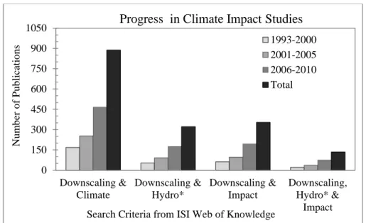
Figure 2.1. Progress in application of downscaling for hydrological impact studies (last accessed Dec 28/2010)
The scientific literatures over the past decade contain large number of reports and reviews detailing the application of hydrologic models to the assessment of the potential effects of climate change on a variety of water resource issues. The intention of this section is thus not to bring all the findings of the researches; rather, to show the attention given to this research area and mapping of the available methodology related to hydrology and water resources. One of the interesting ways to look at the attention given to this area of research is the intense number of progressive articles emerging on downscaling GCMs and RCMs for
0 150 300 450 600 750 900 1050 Downscaling & Climate Downscaling & Hydro* Downscaling & Impact Downscaling, Hydro* & Impact Nu m b er o f P u b licatio n s
Search Criteria from ISI Web of Knowledge
Progress in Climate Impact Studies
1993-2000 2001-2005 2006-2010 Total
hydrological impact studies. Figure 2.1 shows publications on the use of downscaling in climate change impact in hydrology. All of these literatures emerged after the IPCC’s First Assessment Report (FAR) of 1991. In all the search criteria used in ISI Web of Knowledge, the last five years (2006-2010) shows huge number of publications than the first ten years (1991-2000) which indicates that there is high attention given to impact studies. When the search criterion “Downscaling, Hydrol* & Impact” is used, comparatively less number of publications were found. This could indicate that the need of impact studies associated to hydrology is still limited and an ongoing interest among scientific societies. Despite this fact, there were different reviews provided by different authors on the available methodologies since establishment of FAR and new developments. The following consecutive sub-sections will provide a review of some of such literatures.
2.2. Climate Models in Water Resources Studies
2.2.1. GCM for Water Resources Studies
Global Atmospheric General Circulation Models (GCMs) have been developed to simulate the present climate and used to predict future climatic changes. In water resources impact assessment there are varieties of such GCMs’ and RCMs’ outputs at different spatial and temporal resolutions. It is also obvious that GCMs are the only tools that are now days providing dataset in water resources impact studies. Among the total
number of available literatures presented in section 2.1 above majority of the research works focused on the use of GCMs through downscaling and only few studies have focused on the use of the RCMs through a technique called “Model Output Statistics” –MOS, (Maraun et al., 2010). The one that uses RCMs will be discussed in the later section, whereas those based on GCMs will be reviewed in this section.
Before exploring some examples that use GCMs that are used in water resources impact study, we will see some drawbacks. Variables such as runoff, soil moisture, and evapotranspiration are not well represented by GCMs (Loaiciga et al., 1996). The GCMs simulation skills decreases from climate variables to hydrological variables while the hydrological importance increases along the same direction (Xu, 1999a). Further, Xu (1999a) has identified three different gaps in using the GCMs for water resources studies. These are: (i) The spatial and temporal scale mismatches, (ii) The vertical level mismatches, and (iii) The accuracy mismatch. As an additional gap (Loaiciga et al., 1996) has mentioned the issue of feedbacks as hydrologic models are used in offline process modelling and GCMs do not consider lateral transfer of water within the land phase.
Despite all the above drawbacks, there are numerous studies conducted using the available GCMs in different part of the world. For example, to relate GCM hydrologic output to river hydrographs, Liston et al. (1994)
developed a runoff routing model that routes GCM-computed runoff through regional- or continental-scale river drainage networks. By following the basin overland flow paths, the routing model generates river discharge hydrographs that can be compared to observed river discharges, thus allowing an analysis of the GCM representation of monthly, seasonal and annual water balances over large regions. Later, Bergstrom et al. (2001) have used two GCMs: UKMO HadCM2 of the Hadley Centre in Reading and the ECHAM4/OPYC3 of the Max Planck Institute for Meteorology in Hamburg to show the impact of climate change on runoff in Sweden. They analysed changes in runoff totals, runoff regimes and extreme values for six selected basins. Their result shows change in extreme values of runoff can be more critical than mean values. More recently, Lotsari et al.(2010) have used two GCMs (HadCM3 and ECHAM5) to evaluate the impact of climate change on future discharges and flow characteristics of the Tana river in sub-arctic northern Fennoscandia under three different emission scenarios: A1B, A2 and B1. They found projected future increase in both temperature and precipitation which are critical parameters governing future floods and flow characteristics as they control the timing and intensity of flood events in the region. Gao et al., (2010) has also used the same emission scenario to evaluate projected stream flow in the Huaihe River Basin (2010-2100) in china by downscaling ECHAM5 using artificial neural network. There is very few applications of GCMs in impact assessment related water quality; however, Mimikou et al.(2000) have shown that there will be significant water quality impairments because of decreased
stream flows using two GCM based climate change scenarios of transient (HadCM2) and equilibrium (UKHI) conditions in central Greece.
2.2.2. RCM for Water resources Studies
Regional Climate Models (RCMs) are developed based on the same representations of atmospheric dynamical and physical processes as GCMs. They have higher spatial resolution in the order of 10-50km that can cover a sub-global domain. As a result of the higher spatial domain, RCMs provide a better description of orographic effects, land-sea surface contrast and land-surface characteristics (Christensen and Christensen, 2007a). Moreover, they enhance the simulation of atmospheric circulations and climatic variables at fine spatial scales which shows their improved ability to reproduce present day climate (Xu, 2000). However, there is still some limitations (Xu, 2000; Hay and McCabe, 2002; Varis et al., 2004) such as: (i) the inheritance of systematic errors in the driving fields provided by global models, (ii) lack of two-way interactions between regional and global climate (iii) the algorithmic limitations of the lateral boundary interface (iv) computationally demanding, and (v) further downscaling requirement for impact studies.
There are many different RCMs currently available, for various regions, developed at different modelling centres of the world. However, the uncertainty issues remains another drawback in use of RCM. Due to this fact, several international efforts have been taken to quantify uncertainties
through model intercomparison. Some of these include the project work in European region: PRUDENCE [Prediction of Regional scenarios and Uncertainties for Defining EuropeaN Climate change risks and Effects] (Christensen and Christensen, 2007a) and ENSEMBLES; and in North America the NARCCAP (North American Regional Climate Change Assessment Program). More recently, a new project called CORDEX (Coordinated Regional Climate Downscaling Experiment) has been initiated by the world climate research program simulations at 50km resolution for multiple regions.
Due to the availability of numerous numbers of such RCMs a number of studies have been conducted in the past. Teutschbein and Seibert (2010), Teutschbein et al., (2011), and Teutschbein and Seibert, (2012) provided a recent review on the use of RCMs for hydrological models. They recommend that a bias correction is necessary for using the outputs in any hydrological models as RCMs are susceptible to systematic model errors caused by imperfect conceptualization, discretization and spatial averaging within grid cells. These biases are typically due to the occurrence of too many wet days with low-intensity rain or incorrect estimation of extreme temperature in RCM simulations. Bias correction is also recommended by Wilby et al.(2000) and Wood et al., (2004) as a minimum requirement when using RCM outputs in hydrological impact studies. However, (Ehret et al., 2012) have the opinion not to misuse the . available methods which may add up the uncertainties in impact assessment.
The uses of RCMs are most often applied in European river basins. Some of the examples are the studies of the effects of climate change on groundwater assessment (Roosmalen et al., 2007), run-off estimation (Rigon et al., 2007), flood risk assessment (Fowler and Wilby, 2010), precipitation, potential evapotransipiration estimation (Baguis et al., 2010), overall catchment scale hydrologic processes (Senatore et al., 2011) . All these assessments are conducted through further downscaling (bias correction) of RCMs. Wood et al.(2004), have applied six approaches for downscaling climate model outputs for use in hydrologic simulation with particular emphasis on each method’s ability to produce precipitation and other variables used to drive hydrologic model. Of the six approaches the Linear Interpolation (LI), Spatial Disaggregation (SD), and Bias Corrected Spatial Disaggregation (BCSD) were applied to RCM to evaluate the climate impact on British Colombia River Basin. Their result showed the BCSD method yielded the only consistently plausible stream flow simulations, whether or not dynamical downscaling was used. Graham et al.(2007a) has also used two bias correction methods (i.e. delta approach and scaling approach) to evaluate the impact of climate change on the hydrology of northern Europe using seven ensembles of RCMs and two GCM scenarios, The two methods gave a similar mean results, but considerably different seasonal dynamics. Hence it can be concluded that the problem of stationarity remains unsolved where extreme conditions are not taken into account. As a means to
overcome such error, Seguí et al.(2010) have used the quantile-mapping method to evaluate the uncertainty related to the downscaling and bias-correction. In order to provide optimized climate scenarios for climate change impact research, Themeßl et al. (2010) have proposed merging of linear and nonlinear empirical-statistical techniques with bias correction methods and investigated their ability for reducing RCM error characteristics. They also found that quantile mapping shows the best performance, particularly at high quantiles, which is advantageous for applications related to extreme precipitation events.
2.2.3. Scale issues in water resources modelling and climate change impact studies
In dealing with processes in a given watershed, conditions are often different in their space or time scale. As stated by Bloschl and Sivapalan, (1995); and Skøien et al.,(2003), hydrological processes occur at a wide range of scales, from unsaturated flow in a 1 m soil profile to floods in river systems of a million square kilometres; from flash floods of several minutes duration to flow in aquifers over hundreds of years. These processes may take place over a shorter time span whereas their estimates may be needed for very long times (eg. the impact of climate change on a water resource of a watershed in the next 100 years). Conversely, the large-scale models and data are used for small-scale predictions (eg. Climate model outputs for event studies). Such differences in time scale involve some sort of extrapolation, or transfer of information across
scales. This transfer of information is called scaling and the problems associates with it are scale issues (Bloschl and Sivapalan, 1995). Both the spatial and temporal scale dilemma in applying hydrological models in impact studies is described in (Schulze, 1997). They are grouped under any of the four categories: (i) The spatial and temporal scale mismatches between GCMs and Catchment models, (ii) The precipitation response mismatch between GCM output and its hydrological importance, (iii) The means vs. variability paradox, and (iv) The transient/invariate climate control paradox.
The scale issue is not only limited to the characteristic time length as spatial variability are also one of the issues in hydrological processes. For example in using climate data for hydrological study bridging the gap between the resolution of climate models and regional and local scale processes represent a considerable problem for the impact assessment. The technique to bridge this gap is known to be downscaling. Overviews of downscaling methods are well summarized in Fowler et al. (2007) including their advantages and disadvantages (refer section 2). As means of scientific approach to overcome the scale issue, it has been discussed in many studies through up-scaling (distributing and aggregating) or downscaling (disaggregation and singling out) processes. The reviews of some of these studies were given in (Rigon et al., 2007; Loaiciga, 2009).
2.3. Known Methodologies for Climate Change Impact
Assessment
One of the earliest review of techniques used for assessing the effect of climate change on water resources is provided by Leavesley (1994). Their review showed a clear image of types of models used in impact studies and problem areas related to number of modelling issues. The issues could be parameter estimation, temporal and spatial scale of application, validation, climate scenario generation, data and modelling tools. Future solutions to such issues are recommended to bring a way for quantitative determination of climate impacts.
The methodologies and major steps for assessing hydrological response to global climate change were explained in detail in (Schulze, 1997; Xu, 1999a; Xu and Singh, 2004; Xu et al., 2005) and their summary is given in the following section. Clear diagrammatic representations of the methodologies were described by different authors (e.g.Loaiciga et al., 1996; Xu and Singh, 2004) and the one by Xu and Singh, (2004) is used for detailed explanation in this short review.
2.3.1 The direct use of GCM outputs in hydrological models
The approach is to directly use the GCM-derived hydrological output since the GCM is the only available tool for detailed modeling of a future climate (Xu et al., 2005). A GCM has four interactive models:
atmospheric, land surface, ocean and sea ice that are expected to produce all the processes to represent the water cycle.
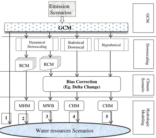
Figure 2.2. Schematic representation of the methods for assessing water resources under changing climate (Source:- Xu and Singh, 2004). In the figure,
GCM is the Global Circulation Model, RCM is the regional climate model, MHM is the macro scale land-surface hydrological model, MWB is the macro scale water balance model, and CHM is the catchment-scale hydrological model. The numbers in circle indicate the individual methods.
2 1 3 4 5 Emission Scenarios GCM Bias Correction (Eg. Delta Change) Dynamical
Downscaling Hypothetical
Water resources Scenarios
RCM RCM Statistical Downscal ing MHM MWB CHM CHM G CM D o w n sc alin g Clim ate S ce n ario H y d ro lo g ic M o d eli n g
However, direct representations of hydrological quantities are highly simplified large- scale averages with little spatial reliability or relevance to specific regions as GCMs were not originally designed for climate change impact studies in hydrology. They thus reflect inherent GCM shortcomings such as runoff being calculated as a secondary variable and not a first-order GCM variable such as P, T, wind or vapor pressure. This process is explained in the diagram (figure-2.2) with the first step labelled with number 1.
2.3.2. Coupling GCMs and Macro-Scale Hydrologic Models
As stated in method i), the GCM does not give a good estimates of hydrologic responses of climate changes. Hence there is a need to couple hydrological models with GCM. Some of the research work done in different part of the world were reviewed by Xu, C.(1999) and Xu et. al., (2005). The results of the studies showed that coupling the hydrological model (macroscale or global) with GCM produces a better representation of the recorded flow regime than GCM predictions of runoff for very large river basin. The examples of such models are: MacPDM (Arnell, 2004), WBM (Vorosmarty et al., 2000) and WaterGAP(Alcamo and Henrichs, 2002). The main theoretical limitations of this method are given in (Hay and McCabe, 2002; Varis et al., 2004) and they are summarized in Xu et al., (2005) as listed below.
i) The inheritance of systematic errors in the driving fields provided
by global models (Loaiciga et al., 1996).
ii) Lack of two-way interactions between regional and global climate.
This limitation is considered as a problem associated with feedbacks by Loaiciga, H. et al., (1996).
iii) Algorithmic limitations of the lateral boundary interfaces
iv) RCM simulations can be computationally demanding depending on
the domain size and resolution (however in recent days this effects are better understood)
v) The need of downscaling (will be explained later) will remain for
individual site impact studies (Wilby and Wigley, 1997; Xu, 1999a)
This method explicitly indicates that simulation of water resources response to climate change is carried out based on hydro-climatic data from GCMs or RCMs and the study focuses more on the world’s largest water bodies. However, Arnell (2004) stated that the macro-scale models are characterized by: their transferability from one geographical location to another, they should be applied either to every sub-basin in the spatial domain or on a regular grid, and runoff must be routed from the point of generation through the spatial domain along the river network. According to the review by Xu et al (2005), the coupled modeling of the atmospheric and hydrological processes is proved to be a powerful tool to study the spatial and temporal evolution of the water and energy budgets of a basin. However, the main problem in using such methods is that the models
need large amount of hydroclimatic and topographic data for calibration that may not available everywhere. The methods of coupling GCM (RCM) with macro-scale hydrologic models are shown in the diagram, (see figure-2.2) with the label numbers 2 and 3.
2.3.3. Downscaling GCM to Force Hydrological Models
Hydrological models require input data (such as precipitation and temperature) at smaller sub-grid scale, which has to be provided by converting the GCM outputs into a reliable time scale for the study area under consideration. However, due to the limitations of GCMs related to the scale issue, an alternate way of using direct GCM-derived hydrological outputs is to downscale the GCM climate outputs for use in hydrological models.
To date, there are different techniques for downscaling large-scale GCM outputs to small-scale resolutions in order to use in impact models. All the available techniques and rationale of downscaling are categorized under two broad groups namely: dynamic downscaling and statistical downscaling techniques (Wilby and Wigley, 1997; Xu, 1999 ; Fowler et al., 2007 are among other reviews).Common to all downscaling methods, Maraun et al., (2010), has provided the most recent review on the application of downscaling techniques for precipitation considering the interest of end users. The most widely used and available techniques
under each category are summarized in the literatures stated above and the relevant information are extracted in the following section.
Dynamic Downscaling
It refers to the use and extraction of local scale information from large scale GCM data using regional climate model (RCM) or limited-area models (LAMs) at 0.5o 0.5o or even higher resolutions that parameterizes the atmospheric processes. They utilize large-scale and lateral boundary conditions from GCMs to produce higher resolution outputs required by hydrologic models. However, the computationally expensiveness of the dynamical downscaling method limits its applicability to smaller time slices; normally ~30 years (eg. from 1961-1990 for control or ‘baseline’ climate and from 2070-2100 for a changed climate used in PRUDENCE) which in turn brought difficulty to assess climate change impacts for other periods (Fowler et.al., 2007).
Statistical Downscaling
In this method, the large-scale atmospheric variables eg. Sea-level pressure and geopotential heights) are empirically related to the local or station-scale atmospheric variables (eg. average precipitation or temperature). The large-scale atmospheric variable are commonly referred to as the predictors whereas the local scale climate variables are the
predictands. According to this method, the predicatnd-predictor relationship can be given using equation-1 below which could be a stochastic or deterministic representation of their relation.
X
F
R
... (1)Where:
R=Predictand (local climate variable that is being downscaled). F= A deterministic or stochastic function that relates the two and
is typically established by training and validating historical point observation or reanalysis data.
X= Predictors (Set of large-scale climate variables)
From equation-1 above the success of the downscaling method is dependent on the relationship used and choice of predictor variables and their performance can be evaluated through quantification of error in mean and explained variances (Khan et al., 2006). The underlying principle of all the statistical downscaling methods is that regional (local scale) climates are however largely a function of the large-scale atmospheric state. The key assumptions (von Storch et al., 2000; Fowler et al., 2007; Maraun et al., 2010) of this method include: (a) the predictors are variables of relevance and are realistically modeled by the GCM, (b) the transfer function is valid also under changing climate conditions (may not be provable) and, (c) the predictors employed fully represent the climate change signal.
All the statistical downscaling methods are categorized under the following three sub group. The description of each method is given in numerous reviews and project papers (Xu, 1999; Fowler et al., 2007; Rigon et al., 2007).where the summary of them are explained as follows.
a. Transfer Functions: in this method, a direct quantitative relationship
between predictand and set of predictors are derived using a linear or nonlinear formulation. Some of the methods that are included under this category are: multiple linear regression methods (eg. Wilby et al., 2002), Canonical Correlation Analysis – CCA (eg. Zorita and von Storch, 1999), Artificial Neural Network – ANN (eg. Coulibaly et al., 2005) and Principal Component Analysis – PCA approaches (eg. Palatella et al., 2010). Among others, the multiple linear regression method, is used to establish regression equation through calibration and validation of local scale climate variables and observed atmospheric predictors for the current climate. For downscaling purpose, the change factors (commonly called as ‘delta changes’) (Prudhomme et al., 2002) calculated based on the GCM outputs are applied to the established regression models. However, it has to be noted that the change factors used in the regression model disregards variability and regression models are only able to capture part of this variability. As a means to overcome such problems, Prudhomme et al. (2002) proposed that any increase in precipitation is distributed evenly among existing rain days that could make each third dry day wet or
distributed on only the three wettest days to simulate an increase in extremes. Other approaches to account variability in regression based downscaling are (i) variable inflation (Karl et al., 1990) that increases variability by multiplying by a suitable factor, (ii) randomization (von Storch et al., 2000) where additional variability is added in the form of white noise, and (iii) expanded downscaling like that of CCA.
b. Stochastic Weather generators (WGs): Stochastic weather
generators like WGEN (Richardson, 1981), LARS-WG (Semenov and Barrow, 1997), GiST (Baigorria and Jones, 2010) are numerical models that generate random numbers realistically looking at sequences conditioned upon the large-scale weather of dry or wet states. These random numbers are expected to have identical statistical properties to that of observed weather. The fundamental principles of weather generators are either based on the Markov chain approach (Hughes et al., 1999; Bellone et al., 2000) or spell-length approach (Wilks and Wilby, 1999b). In Markov chain approach, a random process is constructed which determines a day at a station as rainy or dry, conditioned upon the state of the previous day, following given probabilities. If a day is rainy, then the amount of rainfall is drawn from yet another probability distribution (e.g., Gamma distribution). One of the drawbacks of this method (eg. First order Markov) is that the probability of precipitation depends only on whether precipitation occurred on the previous days that may produce synthetic series exhibiting very long dry spells too frequently (Wilks, 1999). However,
in case of spell-length approach, instead of simulating precipitation occurrences day by day, the models operate by fitting probability distribution to observed relative frequencies of wet and dry spell lengths.
Weather Generators are originally developed to serve for two main purposes (Semenov et al., 1998). The first one is the provision of weather data time series long enough to be used in an assessment of risk in hydrological or agricultural applications. The second purpose is to provide the means for extending the simulation of weather to locations where observed data is not available. In addition to these purposes, weather generators have got due attention in climate change studies as they can serve as a computationally inexpensive tool to produce site-specific climate change scenarios at the daily time-step. For the latter purpose, the changes in the simulated results of GCM scenarios can be applied to the parameters of the weather generators that are derived using observed data (mainly precipitation, maximum temperature, minimum temperature and radiation). The Long Ashton Research Station Weather Generator (LARS-WG) is among the types of weather generators widely applied in downscaling climate GCM datasets for impact studies.
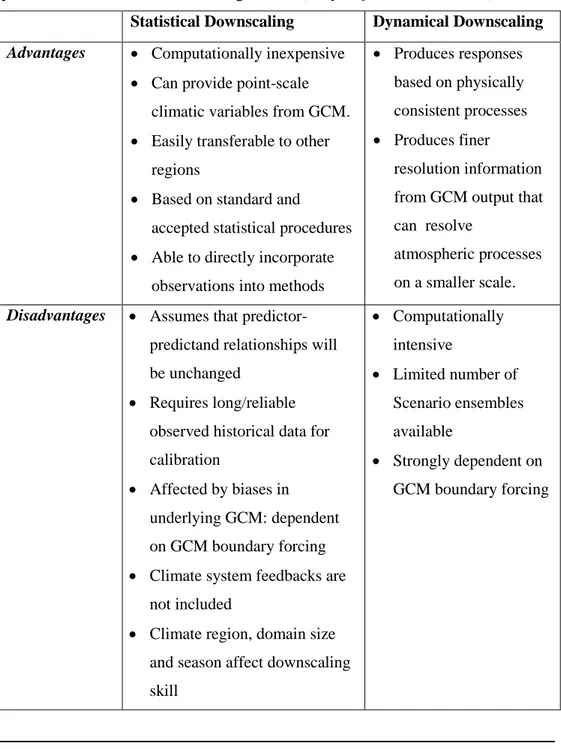
Table 2.1: Comparative summary of the relative advantages and disadvantages of dynamical and statistical downscaling method (adapted from Fowler, 2007)
Statistical Downscaling Dynamical Downscaling
Advantages Computationally inexpensive
Can provide point-scale climatic variables from GCM.
Easily transferable to other regions
Based on standard and
accepted statistical procedures
Able to directly incorporate observations into methods
Produces responses based on physically consistent processes
Produces finer
resolution information from GCM output that can resolve
atmospheric processes on a smaller scale.
Disadvantages Assumes that predictor-predictand relationships will be unchanged
Requires long/reliable observed historical data for calibration
Affected by biases in underlying GCM: dependent on GCM boundary forcing
Climate system feedbacks are not included
Climate region, domain size and season affect downscaling skill Computationally intensive Limited number of Scenario ensembles available Strongly dependent on GCM boundary forcing
c. Weather Typing: is based on the more traditional synoptic
climatology concept (including analogs and phase space partitioning) and which relate a particular atmospheric state to a set of local climate variables. This scheme define empirically weather classes (synoptically or by constructing indices of airflow) related to regional climate variations. This includes analog method and classification tree analysis and it assumes that the weather classes will not change.
Given the range of downscaling techniques and the fact that each approach has its own merits and demerits, there exists no universal method which works for all situations to date. However, it is recommended that rigorous testing and model inter-comparison will have paramount benefit for the reliability of the final results of climate change impact assessments.
2.3.4. Using hypothetical scenarios in Hydrological Models
This method is also known as the delta change or simple alteration method and widely used in almost all part of the world (e.g., Loaiciga, 2009; Xu, 2000; Roosmalen et al., 2010, are few among the know research works).
The general procedure for estimating the impacts of hypothetical climate change on hydrological behavior has the following stages (Loaiciga et al., 1996; Xu, 1999): (i) Determination of parameter values of a hydrological