Coupled lithosphere-mantle dynamics and surface responses: insights from modeling

(1)

COUPLED LITHOSPHERE-MANTLE DYNAMICS AND

SURFACE RESPONSES: INSIGHTS FROM MODELING

PhD. Thesis

by Flora Bajolet

presented at “University Roma Tre”

in the section Geology of the Environment and Geodynamics

(Geologia dellʼAmbiente e Geodinamica, XXV ciclo)

Under the supervision of

Claudio Faccenna and Francesca Funiciello

External reviewers:

Dimitrios Sokoutis – University of Utrecht (The Netherlands) Laurent Husson – University of Rennes 1 (France)

(2)

Abstract

The focus of this work is to understand the interaction in space and time between mantle and lithosphere under different conditions. In a first part, I explore the behavior of the lithosphere under a vertical surface load whilst a second part deals with deep lithospheric load. The third chapter presents preliminary results on dynamic topography in subduction zone. Finally, in a fourth chapter I investigate the surface evolution under kinematically imposed convergence. The adopted methodology consists in scaled analog experiments simulating the lithosphere and upper mantle, during which mantle flow, kinematics, surface topography and deformation can be recorded. The results are then compared with numerical simulations and natural data. Surface loading/unloading experiments using a visco-elastic lithosphere show that we can simulate isostatic rebound using layers of silicone putty and gelatin. Reequilibration occurs in two phases: a fast elastic reequilibration at the My time-scale, and a slower viscous response spanning over tenth of My.

The presence of a deep lithospheric load is modeled by a thick lithospheric root inducing continental delamination. This process produces a complex topographic signal combining isostasy, flexure and dynamic topography coupled with mantle flow and surface deformation. The performed experiments provide a first order quantification of the forces at work alongside with empirical constrains.

The third part aims at modeling subduction zone and tracking dynamic topography, especially in the overriding plate.

Results of the fourth part of this work show that kinematically imposed convergence during subduction and collision can lead to the formation of a curved orogen with various topographic patterns. In that case, strength of the subduction fault zone, rheology of the upper plate and boundary conditions are the most important parameters controlling mantle-lithosphere interactions.

(3)

- Hydrostatic, where the compensation is determined by the topographic load [Airy model, 1855]. The principle is to do a vertical balance of stresses, the lithosphere is assumed to have zero strength, and such methods are valid for large regions [Turcotte and Schubert, 1982]. - Flexural models where the lithosphere is considered as a layered body with visco-elastic behavior. This method takes into account horizontal elastic stresses, and can thus be applied both in 2D or 3D.

Flexure of the lithosphere has an important impact on surface topography in numbers of geologic contexts such as volcanic seamounts loading, bending of passive margins, foreland basins, or post-glacial rebound. Several analytical or numerical models have been performed in the last decades, but analog approach has not been deeply explored.

Additionaly, a dynamic component of can be added to the topography: it corresponds to the part of the signal responding to stresses arising from the mantle [e.g. Colin and Fleitout, 1990; Conrad and Husson, 2009; Moucha et al., 2008]. Especially, dynamic topography in subduction zones have been investigated as it can produce cahnges in elevation of the order of kilometers [e.g. Gurnis, 1990b, 1992; Mitrovica, 1996; Liu et al. 2008; Guillaume et al., 2009; Faccenna and Becker, 2010; Husson et al., 2012; Melosh and Raefsky, 1980; Zhong and Gurnis, 1994; Husson, 2006].

However, in most cases, it difficult to distinguish the effects if isostasy, flexure and dynamic topography. In the following chapters, we will investigate several geodynamic contexts and try to decipher the relationships between deep processes and surface responses, both topography and deformation.

Airy, G.B. (1855). On the computation of the effect of the attraction of mountain-masses as disturbing the apparent astronomical latitude of stations in geodetic surveys. Philosophical Transactions of the Royal Society of London, 145, 101–104.

(7)

Colin, P., and L. Fleitout (1990). Topography of the ocean floor: thermal evolution of the lithosphere and interaction of deep mantle heterogeneities with the lithosphere. Geophysical Research Letters, 17, 1961–1964.

Conrad, C.P., and L. Husson (2009). Influence of dynamic topography on sea level and its rate of change. Lithosphere, 1, 110–120.

Faccenna, C., and T.W. Becker (2010). Shaping mobile belts by small-scale convection. Nature, 465, 602–605.

Funiciello, F., M. Moroni, C. Piromallo, C. Faccenna, A. Cenedese, and H.A. Bui (2006). Mapping mantle flow during retreating subduction: laboratory models analyzed by feature tracking. Journal of Geophysical Research, 111, 3402.

Guillaume, B., J. Martinod, L. Husson, M. Roddaz, and R. Riquelme (2009). Neogene uplift of central eastern Patagonia: dynamic response to active spreading ridge subduction? Tectonics, 28, C2009.

Gurnis, M. (1990b). Ridge spreading, subduction, and sea level fluctuations. Science, 250, 970–972.

Gurnis, M. (1992). Rapid continental subsidence following the initiation and evolution of subduction. Science, 255, 1556–1558.

Husson, L. (2006). Dynamic topography above retreating subduction zones. Geology, 34(9), 741-744.

Husson, L. (2012), B. Guillaume, F. Funiciello, C. Faccenna, and L.H. Royden. Unraveling topography around subduction zones from laboratory models. Tectonophysics, 526-529, 5-15.

Liu, L., S. Spasojević, and M. Gurnis (2008). Reconstructing Farallon Plate subduction beneath North America back to the Late Cretaceous. Science, 322, 934-938.

(8)

Melosh, H.J., and A. Raefsky (1980). The dynamical origin of subduction zone topography. Geophysical Journal, 60, 333–354.

Mitrovica, J. (1996). The Devonian to Permian sedimentation of the Russian Platform: an example of subduction-controlled long-wavelength tilting of continents. Journal of Geodynamics, 22, 79–96.

Moucha, R., A.M. Forte, J.X. Mitrovica, D.B. Rowley, S. Quéré, N.A. Simmons, and S.P. Grand (2008). Dynamic topography and long-term sea-level variations: there is no such thing as a stable continental platform. Earth and Planetary Science Letters, 271, 101–108.

Stüwe, K. (2002). Geodynamics of the Lithosphere. Springer, Berlin, 449pp.

Turcotte, D.L., and G. Shubert (1982). Geodynamics: Application of Continuum Physics to Geological Problems. Wiley, New York, NY 450pp.

Watts, A.B. (2001). Isostasy and Flexure of the Lithosphere. Cambridge University Press, Cambridge, UK 478pp.

Zhong, S., and M. Gurnis (1992). Viscous flow model of a subduction zone with a faulted lithosphere: long and short wavelength topography, gravity and geoid. Geophysical Research Letters, 19, 1891–1894.

Zhong, S., and M. Gurnis (1994). Controls on trench topography from dynamic models of subducted slabs. Journal of Geophysical Research, 99, 15683.

(9)

(10)

1. Introduction and purposes

The flexural isostasy arising from the rigidity of the lithosphere and accompanying loading and unloading processes has a major contribution of Earth’s topography. It has been observed in various settings such as loading in volcanic areas or foreland basins, bending of passive margins, or post-glacial rebound. These processes have previously been quantified with analytical and numerical means, but have not been tested with analog models.

The main purpose of this preliminary study is to elaborate an experimental procedure reproducing surface loading/unloading and able to take into account the visco-elastic properties of the lithosphere.

2. Experiments setup

2.1. Rheological properties of the materials

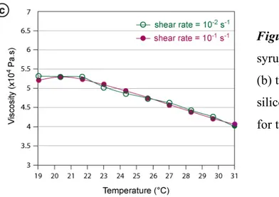
In our models, we use three types of analog materials: glucose syrup, silicone putties and gelatin. The glucose syrup simulating the asthenospheric mantle is a simple Newtonian fluid at experimental strain rates (ca. 10-2 s-1), whose viscosity varies with the temperature (Figure I.1ab). The silicone putty is a visco-elastic material that is considered

quasi-Newtonian at experimental strain rates [Weijermars, 1986], and also shows a dependence on temperature (Figure I.1c).

(11)

Gelatins are also visco-elastic material but with a non-negligible elastic component. The response of these materials to stress is time-dependent and can be characterized measuring the deformation energy stored during deformation and lost afterwards [Mezger, 2002]. If the storage modulus G’ is largely superior to the loss modulus G’’ at a given frequency ω, the material will behave elastically, while in the frequency range where G’’>>G’, it will behave viscously [Figure I.2a; Mezger, 2002]. We use pig skin gelatin powder mixed with water at 2.5%wt and 10°C since it has been shown fitted to model lithosphere rheological behavior [Figure I.2b; Di Giuseppe et al., 2009].

Figure I.2. (a) Evolution of the storage and loss modulus, G’ and G’’ with the frequency ω

for an ideal visco-elastic material. In the visco-elastic domain, G’ and G’’ are of the same order of magnitude. The intersection between the two curves determines the relaxation time of the system (λ) [modified after Di Giuseppe et al., 2009]. (b) G’ and G’’ measured for pig skin gelatin at 2.5%wt and 10°C. The shaded area represents the visco-elastic domain [modified after Di Giuseppe et al., 2009].

Figure I.1. Viscosity of the glucose

syrup depending on (a) shear rate and (b) temperature. (c) Viscosity of the silicone putty depending on temperature for two experimental shear rates.

(12)

2.2. Experimental procedure

We performed two types of models (Figure I.3). In the first type of models, the

lithosphere is modeled by a single layer of silicone and the load is undeformable (Figure I.3a). In the second type of models, we add a thin layer of gelatin on top of the silicone and the load itself is made of deformable gelatin (Figure I.3b). Characteristics of the plates and loads are given in Table I.1. In all cases, the modeled lithosphere is lying on top of low-viscosity glucose syrup simulating the asthenosphere. The bottom of the box represents the 660 km discontinuity. The model is unconstrained in all directions, and no tectonic forces are applied. We place the load at the center of the plate and leave it for 30 min (loading phase), then remove it (unloading phase). This setup implies the following assumptions, and consequent limitations, that are detailed in Funiciello et al. [2003]: (1) isothermal system, (2) constant viscosity and density over the depth of the individual layers, and (3) lack of global

background mantle flow. The topography evolution is monitored with a 3D laser-scanner (Real Scan USB) whose precision is 0.1 mm corresponding to 600 m in nature.

Figure I.3. (a) Experimental setup for the first type of models with a single silicone layer

(brown) and a spherical undeformable load. (b) Models type 2 with silicone and gelatin layers (white) and deformable load.

Parameters Model 1 Model 2

Plate size (cm2) 30 x 30 30 x 30

Silicone thickness (cm) 1.2 1.2

Gelatin thickness (cm) n/a 0.3

Load size diameter 12cm, height 3mm diameter 3 cm, height 2 cm

Load weight (g) 46 11

(13)

3. Preliminary results

All the topographic maps presented thereafter are the difference between two scans and thus represent a difference in elevation (Δz) for a certain time step. The vertical resolution of the scanner is 0.1 mm and variations inferior to that value are background noise.

3.1. Model 1: viscous lithosphere, undeformable load

As soon as the system is loaded, a depression is created in the center edged by a flexural bulge due to the bending of the plate (Figure I.4a). It induces about 1 mm of uplift during the first 10 min of loading. The width of the area affected by the flexural bulge is about one half of the load diameter. The elevation of the rest of the plate remains unchanged. Deformation of the plate continues during the time span 10 to 30 min but with a smaller amplitude (Figure I.4b). In 20 min, the flexural bulge is uplifted by ca. 0.5 mm.

Figure I.4. Map view and corresponding cross-section (along the axe x = -25) of topography

evolution (Δz) for the model 1 during loading phase, (a) for the time step 0 to 10 min, (b) for time step 10 to 30 min. The white circle highlights the position of the load.

(14)

After 30 min, the elevation is stable, and we remove the load. We observe an uplift of the plate, at first with a stronger amplitude in the centre, then propagating in the whole model (Figure I.5). On the contrary, the flexural bulge undergoes subsidence and progressively reequilibrates. The main part of the reequilibration takes place during the first 15 min (Figure I.5a). The variation of elevation from 15 to 45 min is reduced (+/- 0.25 mm; Figure I.5b), and from 45 to 210 min Δz is negligible (+/- 0.15 mm; Figure I.5c). The lateral gradient formed in the late phases of loading and unloading (Figure I.4b and I.5bc) is probably due to the laying and removing of the weight non exactly positioned at the center of the plate and/or disturbance by the operator’s gesture.

(15)

Figure I.5. Map view and corresponding cross-section (along the axe x = -25) of topography

evolution (Δz) for the model 1 during unloading phase, (a) for the time step 0 to 15 min, (b) for time step 15 to 45 min, (c) for time step 45 to 210 min. The white circle highlights the previous position of the load.

This type of model, although made only of silicone putty, shows a non-negligible flexural response to loading/unloading processes. This suggests that the usual approximation of silicone putties behaving as Newtonian fluids [Weijermars, 1986] should be taken with caution. The main part of isostatic reequilibration occurs within 15 min (elastic response) while the last increments of deformation take one to several hours (viscous response).

3.2. Model 2: visco-elastic lithosphere, deformable load

As for the model 1, the response to loading starts as soon as we place the load and lead to the formation of a depression edged by a flexural bulge (Figure I.6a). However, the bulge surrounding the load spread over a larger area than for model 1 (larger wavelength) and is smaller in magnitude with a maximum of 0.5 mm of uplift after 10 min. Isostatic and flexural adjustments continue from 10 to 30 min with 0.2 to 0.5 mm of uplift affecting all the plate’s surface (Figure I.6b).

After 30 min, we remove the load from the plate. The magnitude of the surface response is more important than for the model 1, especially just below the load with an uplift of 3.25 mm in 5 min (Figure I.7a). The flexural bulge has similar values of subsidence, but reequilibration is occurring faster than for model 1 (0.5 mm in 5 min compared to 0.6 mm in 15 min). The isostatic response decreases with time and affects only the very center of the model in the late stages (Figure I.7bc).

Compared to the first type of models, the delay between the applied stresses (loading/unloading) and the surface response is shorter. The elastic component is enhanced by the thin layer of gelatin. As for model 1, the viscous part of the response is spanning over a longer time (one to several hours).

(16)

Figure I.6. Map view and corresponding cross-section (along the axe y = -180) of topography

evolution (Δz) for the model 2 during loading phase, (a) for the time step 0 to 10 min, (b) for time step 10 to 30 min. The white circle highlights the position of the load.

Conclusions and perspectives

The use of silicone putties associated with pig skin gelatin opens new opportunities to adjust the visco-elastic properties of analog materials to natural cases. The gelatin layer increases the elastic response and shortens the delay between applied stresses and surface reequilibration. Varying the thickness of the gelatin layer and using different types of loads would allow modelers to simulate various processes implying flexure and isostatic response.

(17)

Figure I.7. Map view and corresponding cross-section (along the axe y = 180) of topography

evolution (Δz) for the model 2 during unloading phase, (a) for the time step 0 to 5 min, (b) for time step 5 to 15 min, (c) for time step 15 to 45 min. The white circle highlights the previous position of the load.

(18)

References

Funiciello, F., C. Faccenna, D. Giardini, and K. Regenauer-Lieb (2003), Dynamic of retreating slabs: 2. Insights from three-dimensional laboratory experiments, J. Geophys. Res., 108(B4), 2207, doi:10.1029/2001JB000896.

Mezger, T.G. (2002). In: Ulrich, Zorll (Ed.), The Rheology Handbook: For Users of Rotational and Oscillatory Rheometers. Hannover, Germany.

(19)

(20)

CONTINENTAL DELAMINATION

:

INSIGHTS FROM LABORATORY MODELS

Flora Bajolet1*, Javier Galeano2, Francesca Funiciello1, Monica Moroni3, Ana-María Negredo4, Claudio Faccenna1

(1) Dipartimento Scienze Geologiche, Università "Roma TRE", Largo S. L. Murialdo 1, 00146 Rome, Italy. (2)Dpto. Ciencia y Tecnología Aplicadas, EUIT Agrícola, U. Politécnica de Madrid, 28040 Madrid, Spain. (3) DICEA, Sapienza Università di Roma, via Eudossiana 18, 00184 Rome, Italy.

(4) Dpto. Física de la Tierra, Astronomía y Astrofísica I, and Instituto de Geociencias (CSIC-UCM). Facultad de Ciencias Físicas, Univ. Complutense Madrid, 28040 Madrid, Spain.

(21)

Abstract. One of the major issues of the evolution of continental lithospheres is the detachment of the lithospheric mantle that may occur under certain conditions and its impact on the surface. In order to investigate the dynamics of continental delamination, we performed a parametric study using physically-scaled laboratory models. The adopted setup is composed of a three-layers visco-elastic body (analog for upper crust, lower crust, lithospheric mantle) locally thickened/thinned to simulate a density anomaly (lithospheric root) and an adjacent weak zone, lying on a low viscosity material simulating the asthenosphere. The results emphasize the interplay between mantle flow, deformation, surface topography and plate motion during a three-phases process: (1) a slow initiation phase controlled by coupling and bending associated with contraction and dynamic subsidence, (2) lateral propagation of the delamination alongside with extension and a complex topographic signal controlled by coupling and buoyancy, while poloidal mantle flow develops around the tip of the delaminating lithospheric mantle, and (3) a late phase characterized by a counterflow that triggers retroward motion of the whole model. A semi-quantitative study allows us to determine empirically two parameters: (1) an initiation parameter that constrains the propensity of the delamination to occur and correlates with the duration of the first stage, (2) a buoyancy parameter characterizing the delamination velocity during late stages and therefore its propensity to cease. Finally, we point out similarities and differences with the Sierra Nevada (California, USA) in terms of topography, deformation and timing of delamination.

1. Introduction

Continental delamination is presently one of the most discussed geodynamic processes due to its significant impact on the long-term behavior of the continental lithosphere. The concept of continental delamination was first introduced by Bird [1978, 1979], who proposed the hypothesis that along a tectonically stable area, the dense lithospheric mantle could peel away from the crust and sink into the asthenosphere. Delamination is permitted as soon as any process provides an elongated conduit connecting the underlying asthenosphere with the base of the continental crust. The delaminated mantle part of the lithosphere peels away as a coherent slice, without necessarily undergoing major internal deformation, and is replaced by buoyant asthenosphere. To avoid ambiguity, the term ‘delamination’ is used here to indicate

(22)

the process that causes the asthenosphere to come into direct contact with the crust, and the hinge of delamination, where the lithosphere peels off the overlying crust, to migrate laterally. Others processes able to remove a part of the lithosphere such as convective removal of the lithospheric mantle developing from Rayleigh-Taylor instabilities [e.g. Houseman et al., 1981; England and Houseman, 1989] are not considered here.

Delamination has often been proposed to explain different observations such as regional uplift associated with alkaline volcanism, anomalously high heat flow and change of stress field toward extension in various geodynamic contexts: either near a plate boundary (western Mediterranean [Channel and Mareschal, 1989]; Alboran sea [Seber et al., 1996; Calvert et al., 2000; Valera et al., 2008]); for intracontinental zones (Variscan belt [Arnold et al., 2001]; Sierra Nevada in California [Ducea and Saleeby, 1998; Zandt et al., 2004; Le Pourhiet et al., 2006]); plateau interiors (Tibet [Bird, 1978]; Anatolia [Gogus and Pysklywec, 2008a]; Colorado [Bird, 1979; Lastowka et al., 2001; Levander et al., 2011]); or in more complex areas exhibiting unusual intermediate depth seismicity (East Carpathians [Girbacea and Frisch, 1998; Knapp et al., 2005; Fillerup et al., 2010]).

In spite of the popularity of continental delamination, its basic aspects remain poorly studied. For one part because most observables possibly indicating ongoing delamination are indirect ones (tomography, seismicity) [Levander et al., 2011], and some surface features (tectonic, volcanism, topography) could be interpreted as subduction-related signals (i.e. slab roll-back, slab break-off). Moreover, few physical-numerical models have been developed [e.g. Schott and Schmeling, 1998; Morency and Doin, 2004; Gogus and Pysklywec, 2008b; Valera et al., 2008, 2011; Faccenda et al., 2009]. Although these models successfully capture the main features of delamination, they have to deal with difficulties such as numerical instabilities associated with fast deforming bodies and with strong lateral contrasts of viscosity. Unlike subduction, which has been investigated by numerous laboratory studies over the last two decades [e.g. Jacoby, 1980; Kincaid and Olson, 1987; Griffiths et al., 1995; Guillou-Frottier et al., 1995; Faccenna et al., 1996, 1999; Funiciello et al., 2003, 2004, 2008; Schellart, 2004), or convective removal [Pysklywec and Cruden, 2004] very few attempts to reproduce continental delamination with analog models have been made [Chemenda et al., 2000; Gogus et al., 2011].

The main purpose of this study is to investigate the dynamics of continental delamination with laboratory models exploring the influence of various parameters (initial structure, rheological properties), and the relationships between deep dynamics (i.e. mantle

(23)

circulation), surface deformation (i.e. deformation, isostatic reequilibration, dynamic topography), and plate motion.

2. Experimental Setup

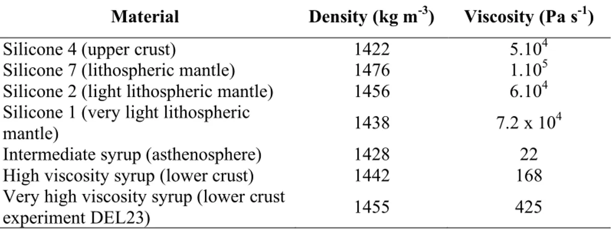
Delamination is reproduced in the laboratory using a thin sheet three-layers model (lithosphere), lying on top of a low-viscosity glucose syrup simulating the asthenospheric mantle (Figure II.1). From top to bottom, the lithospheric sheet is composed of: 1) visco-elastic silicone putty simulating the upper crust, 2) high-viscosity glucose syrup simulating the viscous lower crust, 3) strong and dense visco-elastic silicone, analog of the lithospheric mantle (Table II.1). The selected asthenospheric mantle is a Newtonian fluid whose viscosity allows us to obtain laminar flow in the limit of a small Reynolds number.

Figure II.1. Experimental setup. Material properties are given in Table II.1, and settings for

each experiment in Table II.3.

The three-layered sheet is located in the center of a large Plexiglas tank (75 x 25 x 25 cm3), whose bottom mimics the 660 km discontinuity, and is free to move in all directions (free boundary conditions). The distance between the plate and box sides is set large enough to minimize possible boundary effects [Funiciello et al., 2006].

(24)

Material Density (kg m-3) Viscosity (Pa s-1)

Silicone 4 (upper crust) 1422 5.104

Silicone 7 (lithospheric mantle) 1476 1.105

Silicone 2 (light lithospheric mantle) 1456 6.104 Silicone 1 (very light lithospheric

mantle) 1438 7.2 x 10

4

Intermediate syrup (asthenosphere) 1428 22

High viscosity syrup (lower crust) 1442 168

Very high viscosity syrup (lower crust

experiment DEL23) 1455 425

Table II.1. Material properties. Viscosities are given for room temperature (22°C) and an

experimental strain rate of 10-2 s-1 (scaled for nature).

This experimental setting is properly scaled for normal gravity field to simulate the competition between acting gravitational and viscous resistive forces stored within the mantle and the lithosphere [e.g. Weijermars and Schmeling, 1986; Davy and Cobbold, 1991]. The density and the viscosity ratios between the lithosphere and asthenosphere range between 1.01 and 1.02 and 400 and 3000, respectively. The length scale factor is fixed to 1.2 x 10−7_{so that} 1 cm in the models corresponds to 83 km in nature. Further details on experimental parameters and scaling relationships can be found in Table II.2. The adopted setup implies the following assumptions, and consequent limitations, that are detailed in Funiciello et al. [2003]: (1) isothermal system, (2) constant viscosity and density over the depth of the individual layers, (3) lack of global background mantle flow, (4) 660 km discontinuity as an impermeable barrier. In contrast with Gogus et al. [2011], we do not impose any convergence, nor manually trigger initiation of delamination. Delamination is spontaneously enhanced by the adopted ad hoc initial condition which, in analogy with previous numerical models [Schott and Schmeling, 1998; Valera et al., 2008, 2010], includes a zone of thicker lithospheric mantle (orogenic root, 1.04 cm thick in the reference experiment) adjacent to a weak zone represented by an asthenospheric channel (absence of lithospheric mantle; Figure II.1). This configuration enables the asthenosphere upwelling to replace the delaminated lithospheric mantle. A similar setting has also been adopted in the numerical models of Gogus and Pysklywec [2008b], who considered a flat geometry of the lithospheric mantle, but imposed a local density increase of 100 kg m-3, producing a negative buoyancy similar to our orogenic root. The presence of a local weakened zone is fundamental to trigger delamination in nature.

(25)

This is usually explained as likely related to the presence of free water, which would decrease the pore pressure allowing a reduction in the brittle strength [Schott and Schmeling, 1998], or thermally active areas in response to active mantle upwelling. This weak zone is spontaneously created only in the model developed by Morency and Doin [2004] where strong localized thinning of the lithospheric mantle leads to the formation of an “asthenospheric conduit”.

Parameter Nature Model

g Gravitational acceleration (m s−2) 9.81 9.81 Thicknessa

hl Continental lithosphere (m) 100000 0.012

hasth Upper mantle asthenosphere (m) 660000 0.11

Density

ρl Continental lithosphere (kg m3) 3200 1457

ρasth Upper mantle asthenosphere (kg m3) 3220 1428–1442

ρl /ρum Density ratio 0.99 1.02–1.01

Viscosity

ηl Continental lithosphere (Pa s−1) 1023 7 × 104

ηasth Upper mantle asthenosphere (Pa s−1) 1021 22–168

ηl /ηum Viscosity ratio 102 4 × 102–3 × 103

Dimensionless parameters Equivalence model-nature t° Characteristic time:

(tmodel/tnature) = (Δρgh)lith nature / (Δρgh)lith model × (ηlmodel / ηl nature)

4.02 × 10−12

1 minmodel → 0.473 Mynature 1 hmodel → 28.4 Mynature U° Characteristic velocity:

(Umodel/Unature) = tnature / tmodel × Lmodel /Lnature

29829

1 cm h−1model → 0.29 cm y−1 nature

a_{Scale factor for length L}

model/Lnature = 1.2 × 10−7.

Table II.2. Scaling of parameters for the reference experiment.

Each model is monitored over its entire duration using a sequence of digital pictures taken in lateral and top views. We also record the evolution of the surface topography with a 3D-laser scanner (Real Scan USB) whose precision is 0.1 mm, corresponding to 830 m in nature. The evolution of delamination is monitored by Feature Tracking (FT) image analysis technique on representative experiments. In order to adopt the FT for our models, the glucose syrup is previously seeded with bright reflecting air micro-bubbles used as passive tracers. These bubbles have a diameter less than 1 mm, and consequently its possible influence on the density/viscosity is negligible. Images of the micro-bubbles are recorded by a CCD camera, set to acquire about 2 frames per second in lateral view. FT algorithms provide sparse velocity

(26)

vectors with application points coincident with pixel luminosity intensity gradients characterizing the passive tracers seeding the mantle. This technique permits to obtain a Lagrangian description of the observed velocity field, which is then used to reconstruct instantaneous and time-averaged Eulerian velocity maps (modulus, x-y components, streamlines) through a resampling procedure [see Funiciello et al., 2006 and references therein].

3. Experimental Results

Our models were performed to provide new insights into the mechanical/dynamic behavior of the lithosphere in a delamination process. In particular, we intend to describe and quantify the spatial and temporal evolution of the mantle circulation induced by delamination and the related surface response. Fourteen models out of 26 (Table II.3) have been selected to illustrate the influence of (1) plate thickness, (2) plate viscosity, (3) plate density, (4) presence/absence/size of the asthenospheric channel, (5) presence/absence/size of the lithospheric root, (6) asthenosphere viscosity on the delamination process.

3.1. Evolution of the reference experiment (DEL 10)

All the performed experiments show a typical sequence of deformation, starting from spontaneous delamination to the arrival of lithospheric mantle to the bottom of the box. In this section, we describe the typical evolution of the delamination process as recorded for the reference model DEL10. DEL10 is characterized by thicknesses of 0.375 cm, 0.2 cm and 0.78 cm for the upper crust, the lower crust and the lithospheric mantle, respectively. It includes a zone of 1.04 cm thick lithospheric mantle simulating the orogenic root. The other parameters are listed in Table II.3. The proward direction is defined as the direction of migration of the delamination (toward the right in all the figures), and retroward direction corresponds to the opposite sense (toward the part of the model that does not delaminate, i.e. left in the figures).

(27)

Table II.3. Experimental parameters for each experiment. UC: upper crust; LC: lower crust;

LM: lithospheric mantle; Asth.: asthenosphere. Values in bold italic are the parameters Experiment Plates (size, silicones) Asthenospheric

channel width (w)

Orogenic root

width (W) Layers thickness

DEL10 UC (sil. 4): 30 x 18 cm_{LM (sil. 7): 30 x 14 cm}22 2 cm 3 cm

UC: 0.375 cm LC: 0.2 cm LM: 0.78 cm Root: 1.04 cm DEL11 UC (sil. 4): 30 x 18 cm_{LM (sil. 7): 30 x 14 cm}22 4 cm 3 cm

UC: 0.38 cm LC: 0.2 cm LM: 0.665 cm Root: 1.04 cm DEL12 UC (sil. 4): 30 x 18 cm_{LM (sil. 7): 30 x 14 cm}22 2 cm 3 cm

UC: 0.37 cm LC: 0.2 cm LM: 0.775 cm Root: 0.55 cm DEL13 UC (sil. 4): 30 x 18 cm_{LM (sil. 7): 30 x 14 cm}22 1 cm 3 cm

UC: 0.35 cm LC: 0.4 cm LM: 0.65 cm Root: 0.975 cm DEL15 UC (sil. 4): 30 x 18 cm 2 LM (sil. 7): 30 x 14 cm2 2 cm 1 cm UC: 0.36 cm LC: 0.2 cm LM: 0.675 cm Root: 0.975 cm DEL16 UC (sil. 4): 30 x 18 cm 2

LM (sil. 7): 30 x 14 cm2 2 cm No orogenic _root

UC: 0.275 cm LC: 0.2 cm LM: 0.65 cm DEL17 UC (sil. 4): 30 x 18 cm_{LM (sil. 7): 30 x 14 cm}22 2 cm No orogenic _root

UC: 0.275 cm LC: 0.2 cm LM: 0.68 cm DEL18 UC (sil. 4): 30 x 18 cm_{LM (sil. 1): 30 x 14 cm}22 2 cm 3 cm

UC: 0.325 cm LC: 0.2 cm LM: 0.725 cm Root: 0.970 cm DEL20 UC (sil. 4): 30 x 18 cm2 LM (sil. 7): 30 x 14 cm2

Asth.: high viscosity syrup 2 cm 3 cm UC: 0.340 cm LC: 0.2 cm LM: 0.720 cm Root: 0.940 cm DEL21 UC (sil. 4): 30 x 18 cm 2

LM (sil.7): 30 x 14 cm2 No asthenospheric. _channel No orogenic _root

UC: 0.40 cm LC: 0.2 cm LM: 0.730 cm DEL22 UC (sil. 4): 30 x 18 cm_{LM (sil.7): 30 x 14 cm}22 No asthenospheric. _channel 3 cm

UC: 0.320 cm LC: 0.2 cm LM: 0.760 cm Root: 0.950 cm DEL23 UC (sil. 4): 30 x 18 cm 2

LM (sil.7): 30 x 14 cm2 No asthenospheric. _channel No orogenic _root

UC: 0.325 cm LC: 0.2 cm very high viscosity syrup LM: 0.660 cm DEL24 UC (sil. 4): 30 x 25 cm_{LM (sil.7): 30 x 24.5 cm}22 No asthenospheric. _channel No orogenic _root

UC: 0.350 cm LC: 0.2 cm LM: 0.770 cm

(28)

varying compared to the reference case (DEL10, highlighted in grey). In a few experiments (DEL21, 22, 23), the lithospheric mantle tends to detach from the lower crust along the borders parallel to the length of the model. This is due to the fact that in this area, the layer of lower crust is in contact with the asthenosphere, thus creating a “false” asthenospheric channel. In experiment DEL24, the layer of silicone simulating the lithospheric mantle is larger avoiding the contact. In this case, there is no delamination.

Figure II.2. Side view photos and surface topography for the reference experiment (DEL10)

at three stages of the delamination process: a) 12 min 57s during initiation phase, b) 44 min at the transition between main and final phase, c) 59 min during final phase, with corresponding cross-sections (d) taken along the reference dotted blue line. The high (red)

(29)

circular zones are air bubbles trapped between the layers during the construction of the model. Later experiments free of that experimental bias showed that it does not affect significantly the delamination process.

3.1.1. Initiation of delamination

At the beginning of the experiment, the area above the asthenospheric channel is 0.1 to 0.2 mm higher than the unperturbed area due to the absence of lithospheric mantle, and the area above the lithospheric root is 0.3 mm lower (Figure II.2ad). The edge of the unstable thickened lithospheric mantle slowly starts to peel away from the overlying lower crust alongside the length of the asthenospheric channel and displaces underlying mantle material proward (Figure II.2a). The amount of time necessary to initiate this process is 30 min (corresponding to 14.2 My in nature) in the reference experiment (Table II.4). Concurrently, the difference of pressure at the base of the sinking lithospheric mantle and in the asthenospheric channel produces a clockwise return flow that injects asthenospheric material into the lower crust toward the lithospheric root. This flow remains very modest during all the initiation with a maximum velocity of 3.6 cm h-1 (Figure II.3a). A small amount of extension parallel to the direction of delamination affects the area above the asthenospheric channel, while the rest of the model is globally in contraction, which is stronger above the lithospheric root (Figure II.4a). The depression caused by the pull of the thickened lithospheric mantle progressively narrows and deepens up to 0.9 mm. As subsidence is deforming the model, two bulges due to bending form, one at each side of the depression (i.e. each side of the lithospheric root). They are ca. 0.1 mm higher than the average elevation of the model (Figure II.2ad). Figure II.5 shows the evolution of the elevation for the uplifted bulge located above the asthenospheric channel, and for the depression migrating with the delamination hinge. Figure II.6 shows the evolution of horizontal velocity of both the dynamic depression, that corresponds to the velocity of delamination (in the plate reference frame), and of the whole model (in a fixed external reference frame).

(30)

(Legend on next page) Experiment Difference with reference experiment Duration of

initiation t Duration of main phase wc (cm)

Duration of final stage Root pull Frp (x10-4 N) Initiation parameter I (x10-7 s7 m -3₎ Buoyancy parameter B (x10-10 m4 s4 kg-1) Mean velocity during Stokes’ phase V (x10-5 m s-1)

DEL10 Reference _experiment 30 min _{(14.2 My)} 4 min (34 min after the beginning of the experiment) (1.9 My)

4.8 27 min _{(12.8 My)} 11.46 6.02 6.20 6.13

DEL11 Asthenospheric _{channel twice wider} 25 min _{(11.8 My)} 0 (25 min) 4.6 23 min _{(10.9 My)} 9.77 16.57 5.29 9.85

DEL12 Lithospheric root _{half thick} 60 min _{(28.4 My)} 24.9 min (84.9 min) _{(11.8 My)} 4.4 18.1 min _{(8.6 My)} 6.02 3.23 3.26 4.13

DEL13 Asthenospheric channel twice narrower

30 min

(14.2 My) 17.8 min (47.8 min) (8.4 My) 4.5 22.2 min (10.5 My) 8.69 5.01 4.70 7.15

DEL14 Lower crust twice _thicker 15 min _{(7.1 My)} 5 min (20 min) _{(2.4 My)} 4.9 14 min _{(6.6 My)} 8.95 16.26 9.69 16.6

DEL15 Lithospheric root 3 _{times narrower} 50 min _{(23.6 My)} 22 min (72 min) _{(10.4 My)} 5.1 20 min _{(9.5 My)} 3.10 2.51 1.68 4.02

DEL16 No orogenic root 45 min (21.3 My)

26 min (71 min) (12.3 My)

Variable along the width of the model

17 min (8.0 My)

Variable along the width of the model

DEL17 No orogenic root 60 min _{(28.4 My)} 37 min (97 min) _{(17.5 My)} 4.7 17 min _{(8.0 My)} Variable along the _{width of the model}

DEL18 Density contrast 4.8 _{times smaller} No _delamination 1.99 0.070 1.07

DEL19 Density contrast 2.4 _{times smaller} 1h45 min _{(49.7 My)} 5.5 min (110.5 min) _{(2.6 My)} 3.7 39.5 min _{(18.7 My)} 5.80 2.15 3.14 4.98

DEL20 Asthenosphere 10 _{times more viscous} 2h20 min _{(66.2 My)} 15.9 min (155.9 min) _{(7.5 My)} 4.3 74.1 min _{(35.0 My)} 6.77 0.30 0.48 1.87

DEL21 No asthenospheric channel, no orogenic root

Detachment by setup bias

DEL22 No asthesnopsheric _channel Detachment by _{setup bias} DEL23

No asthenospheric channel, no orogenic root, lower crust more viscous

Detachment by setup bias

DEL24

No asthenospheric channel, no orogenic root, larger plates

No delamination

(31)

Table II.4. Characteristic values of duration and physical parameters for each experiment.

Durations of characteristic phases are given in minutes with the corresponding scaled time for nature (in My). Main phase is defined as the time span between the end of initiation and the onset of retroward motion of the plate, the final phase from this change in kinematics until the DLM touches the bottom of the box. wc is the width of the asthenospheric channel at the

transition between main and final phase. For experiments DEL16 and DEL17, in the absence of lithospheric root, the shape of the delamination hinge is highly sinuous, with very variable velocities of delamination along the width of the model.

Figure II.3. Velocity field (lateral view) for experiment DEL10 at four different stages of the

delamination: a) 30 min just after initiation, b) 39 min at the end of the main phase of delamination, c) 44 min at the change in dynamic with strong increase in retroward motion of the model, d) 59 min during the last phase of delamination, just before the DLM reaches the bottom of the box. Color scale represents the velocity in the x direction (length, positive in the proward direction). Shadowed images underline the position of the model.

(32)

3.1.2. Main phase of delamination

Once the lithospheric mantle decouples from the crust, the hinge of the delamination migrates progressively proward and the dip of the delaminated lithospheric mantle (DLM) increases (Figure II.3b). As the DLM rolls back in the proward direction, the poloidal clockwise flow centered beneath the tip of the slab enhances the ascent of asthenosphere, which replaces the DLM. Maximum velocities of 10.8 cm h-1 are reached soon after the end of the main phase, at 39 min (Figure II.3b). Sinking and proward motion of the DLM enlarge the asthenospheric channel and an ascending asthenospheric counterflow directed retroward grows (Figure II.3c). The initial topographic signal (composed of the depression flanked by the two bulges) moves laterally following the delamination’s propagation with a velocity reaching 8 cm h-1 at 33 min (equivalent to 2.4 cm yr-1 in nature, Figure II.6a), and increases in amplitude. The bulge situated toward the asthenospheric channel is more uplifted than the one on the other side (reaching respectively 0.3 and 0.2 mm; Figure II.2bd) due to the impingement of the ascending asthenospheric material against the base of the crust. The increased bending of the plate causes the formation of a second area of extension above the smaller flexural bulge (Figure II.4b). The area where the lithospheric mantle is removed is also uplifted by 0.1 to 0.3 mm (Figure II.2abd). This elevated zone will remain permanently until the end of the experiment, whereas high and low areas moving with the delamination are the transient, dynamic response of the system.

(33)

Figure II.4. 2D finite strain map of the upper crust (top view) and corresponding side view

photos at 3 different stages of the delamination for experiment DEL13: a) initiation between 0 and 30 min, b) main phase between 30 and 45 min, c) final phase between 45 and 68 min. Finite strain is computed with SSPX software [Cardozo and Allmendinger, 2009]. Initial and final coordinates of reference points drawn on the upper silicone are transformed into a displacement gradient tensor from which is calculated the strain gradient tensor. The deformation field is then computed with a grid-nearest neighbor method.

(34)

Figure II.5. Evolution through time of (a) the amplitude of elevation for the uplifted bulge

and (b) depression migrating with the delamination’s hinge in the plate reference frame (most significant experiments). The curves stop just before the DLM touches the bottom of the box (upper/lower mantle boundary).

Figure II.6. Evolution of (a) the horizontal velocity of the dynamic depression in the plate

referential and (b) the whole model in a fixed external reference frame. The displacement of the dynamic depression follows the delamination front and can be assimilated with the horizontal velocity of delamination. Delamination during experiment DEL17 (without

(35)

orogenic root) is very irregular and it is therefore difficult to measure the displacement of the dynamic depression at the delamination’s hinge.

3.1.3. Final stage

Around 4 min after delamination initiation, i.e. 34 min after the beginning of the experiment, the width of the delaminated area reaches a critical value of ca. 4.5 cm (Table II.4). The pull induced by the DLM triggers the rapid retroward motion of the plate that sharply accelerates up to 12 cm h-1_{at the end of the experiment (3.5 cm yr}-1_{in nature, Figure} II.6b), and enhances the efficiency of the asthenospheric counterclockwise flow (Figure II.3b). The DLM’s proward motion stops although delamination proceeds: the DLM roughly remains in a fixed position with respect to an external fixed reference frame, and delaminates near vertically. The mantle circulation associated with this final stage is thus characterized by the coeval flow of two advection cells, a clockwise cell to the left of DLM and a counterclockwise cell to the right (counterflow).

Consequently to the near-vertical position of the DLM, the hinge of delamination, the associated surface deformation and the topographic signal also remain fixed with respect to an external reference frame. However, they still move proward in the plate’s reference frame, with a maximum velocity of 23 cm h-1 at the end of the experiment (6.8 cm yr-1 in nature, Figure II.6a). Increase in amplitude of both the depression and uplifted bulge continues until the DLM approaches the bottom of the box (Figures II.2cd and II.5). Similarly, the surface above the delaminated area continues to widen and uplift up to 0.2 to 0.3 mm as previously (Figure II.2d). Zones of extension (associated with both bulges) and contraction (associated with the dynamic depression) follow the delamination’s hinge as elastic deformation. The resulting finite deformation for the whole duration of the final phase shows widening of extension both above the delaminated area and the flexural bulge. However, approximately half the delaminated area has undergone finite compression (Figure II.4c). A part of the deformation is elastic and thus transient, but the model is also durably deformed with 6% of shortening accumulated in the whole lithosphere at the end of the experiment.

(36)

Figure II.7. Velocity field for experiment DEL11 (a-d) and DEL12 (e-h) presented as for

(37)

3.2. Sensitivity analysis

We performed a parametric study to test how the initial geometrical configuration and rheological properties of the lithosphere can influence the evolution of delamination. The main features characterizing the delamination process are invariant for all the experiments, but the timescale, mantle flow velocity and amplitude of the surface features depend on the adopted parameters.

Key parameters determining the occurrence and timing of the first phase of delamination are the thickness of the lower crust (i.e. degree of coupling between lower crust and lithospheric mantle), and the width of the asthenospheric channel. Delamination starts earlier and proceeds faster when the lower crust is thicker, and/or the asthenospheric channel is wider (compare in Figures II.5 and II.6 DEL10 with DEL11 and DEL14, Table II.4). Thickness of the orogenic root, alongside with density contrast between the lithospheric mantle and asthenosphere has also an impact on delamination velocity, especially in the initiation phase (compare in Figures II.5 and II.6 DEL10 and DEL19, Table II.4). If the density contrast is very small (<7 kg m-3), the delamination does not initiate (Table II.3, DEL18 not detailed here). A viscosity contrast one order of magnitude lower slows down the whole process, initiation as well as main and final phases of delamination (Tables II.3 and II.4, DEL20 not detailed here).

Although the global pattern of mantle flow is stable whatever the parameters are, the timing of the different phases and flow velocities vary. If the asthenospheric channel is initially two times larger (4 cm instead of 2 cm, DEL 11, Figure II.7a), delamination is slightly faster during the whole modeling evolution (Table II.4). More precisely, mantle flow is slower during the main phase of delamination (with a maximum of 8.1 cm h-1 against 10.8 cm h-1 for reference experiment; Figure II.7b), followed by a faster final phase (9 cm h-1 against 7.2 cm h-1, Figure II.7d). When the orogenic root is half thick (0.55 cm instead of 1.04 cm, DEL12, Figure II.7e to h), we do not observe clear distinct phases but rather a continuous increase in flow velocity, more significant after the retroward plate motion has started (Figure II.7gh). However, this result must be taken with caution given that in this experiment, the delamination front is twisted and does not allow a good view for mantle flow record.

The topographic signal results from the interplay between different parameters, with a dominant role played by the gravitational instability of the lithospheric root. The amplitude of the topography (both for the depression and the uplifted bulge) is higher for a thick and dense lithospheric root, which therefore creates a stronger relief (Figure II.5, compare DEL10, DEL12, DEL 17 and DEL 19). On the contrary, a lower viscosity contrast between

(38)

lithosphere and asthenosphere results in lower amplitude of topography (Table II.3, DEL20 not detailed here).

Geometry and propagation of delamination is controlled by the presence/absence and size of the orogenic root. In experiments where the lithospheric root is absent (Table II.3 and Figure II.5, DEL17 and DEL16, not detailed here), delamination begins strongly delocalized along the asthenospheric channel and, afterwards, irregularly propagates in several directions. As a consequence, the topographic signal following the delamination is also heterogeneous in shape and amplitude.

4. Discussion

All the parameters discussed below are listed with symbols and units in section 8. 4.1. Forces at work during delamination

A typical feature of delamination, compared to convective removal, is that the lithospheric mantle delaminates coherently, with little internal deformation and with a geometry comparable to that of a subducting lithosphere. Thus, the following analysis of forces acting during the delamination process is partly inferred from previous studies on subduction [e.g. Forsyth and Uyeda, 1975; Turcotte and Schubert, 1982; Conrad and Hager, 1999; Funiciello et al., 2003; Lallemand et al., 2008].

The main driving force is the gravitational instability generated by the presence of the lithospheric root that progressively pulls down the lithospheric mantle. The root pull (Frp)

increases with time as more lithospheric mantle is delaminated. In analogy with the slab pull [e.g. Forsyth and Uyeda, 1975; McKenzie, 1977; Davies, 1980], our root pull force can be expressed as

Frp= ΔρghLMWH (1)

where Δρ is the density contrast between the lithospheric mantle and the asthenosphere, g the gravity acceleration, hLM is the thickness of the delaminated lithospheric mantle and W and H

the width and thickness of the lithospheric root respectively.

The resisting forces include the shear resistance at the lower crust/lithospheric mantle boundary, the bending resistance, and the asthenosphere resistance at the interface with the DLM. First, the lithospheric mantle has to overcome the coupling (i.e. the shear resistance) with the lower crust. The shear stress at the base of the lower crust τLC is proportional to the

(39)

τLC = ˙γ ηLC (2)

The lower crust deforms by a combination of Couette and Poiseuille flow. However, side view photos show a pattern closer to Couette flow’s geometry at the base of the lower crust, consistent with the deformation observed in numerical models [Le Pourhiet et al., 2006]. Therefore, we will approximate the shear rate at the first order as Couette flow in a Newtonian fluid so that

˙γ = v/hLC (3)

where v is the velocity in the lower crust and hLC its thickness. Expressions (2) and (3) give

τLC = v ηLC/hLC (4)

The delamination process requires bending of the lithospheric mantle. Following Turcotte and Schubert [1982], the force necessary to bend a viscous layer can be approximated by

Rb ≈ VdhLM3ηLM/r3 (5)

where Vd is the velocity of delamination, ηLM and r the viscosity and radius of curvature of the

lithospheric mantle respectively.

The displaced asthenosphere also exerts a viscous resistance on the DLM at its interface. For subduction, this resistance has been solved with fluid dynamics equations for the case of a stationary slab [Turcotte and Schubert, 1982]. Following the simplification adopted by Funiciello et al. [2003], we will only estimate the order of magnitude. At the first order, the viscous shear resistance is proportional to the asthenosphere viscosity ηasth and

velocity of delamination Vd

Rasth ∝ ηasthVd (6)

Acceleration of delamination with time implies a faster increase of the driving force (root pull) compared to the resisting forces. Indeed, the bending resistance decreases rapidly as it is inversely proportional to the cube of the radius of curvature expressed as the deviation of the initial straight shape. The shear resistance at the base of the lower crust and the viscous resistance of the asthenosphere, tough increasing with the velocity in the lower crust and the velocity of delamination respectively, do not compensate for the augmentation of the root pull force. In the following section, we examine the evolution of the forces at work with time and their influence on the observables (timing, velocities, topography) and attempt to further quantify the delamination process.

(40)

4.2. Dynamics of delamination and surface response

The initial configuration is unstable due to the negative buoyancy of the lithospheric mantle. Conditions for initiation include a sufficient root pull: if Frp < 2 x 10-4 N (experiment

DEL18) the process does not start within the time span tested in laboratory (4 hours equivalent to 113.5 My). The mantle flow generated in the asthenospheric channel is very modest and is due to the difference of pressure between the asthenospheric channel and the base of the heavy lithospheric root. Injection of asthenospheric material at the extremity of the lithospheric root causes a viscosity decrease in the area previously occupied by the lower crust. Progressive sinking of the root enlarges the conduit. Consequently, the shear resistance τLC (equation 4) is reduced with relative increase of the root pull force’s efficiency. This is

indeed confirmed in experiment DEL14: when the lower crust is twice thicker, the time required for initiation is twice shorter (Table II.4, Figures II.5 and II.6). A wider asthenospheric channel (DEL11) allows for a stronger initial mantle flow that also reduces slightly the duration of initiation phase (Table II.4, Figures II.5 and II.6). In order to determine the main parameters controlling the initiation phase, we consider two parameters: the ratio T° between the time required for initiation (t) and the total duration of the experiment (T):

T° = t/T (7)

and an initiation parameter (I) representing the ratio of driving forces over resisting forces acting during initiation such as

I = Frp/τLCRbRasth (8)

I will successfully represent the possibility for delamination to initiate if it correlates well with T°. We can therefore try to adjust its expression empirically. In equations (4), (5) and (6), we observe that τLC, Rb and Rasth are proportional to ηLC/hLC, ηasth and hLM3ηLM, respectively,

then

I ∝ FrphLC/ηLCηasthhLM3ηLM (9)

Moreover, the width of the asthenospheric channel, not taken into account in the force balance analysis, is a parameter enhancing the velocity of the initiation phase and hence can be placed at the numerator. The best fit between I and T° is obtained by adding a factor Δρ2 that highlights the strong dependency of the initiation duration on the density contrast so that

(41)

Figure II.8 shows a good linearly inverse correlation between I and T°, highlighting how I and, in turn, the interplay between its constitutive parameters, reasonably characterizes the possibility for the delamination to initiate.

Figure II.8. Plot of the initiation parameter (I) versus the ratio between the time required for

initiation of delamination and the total duration of the experiment (T°) with best fit regression line. The regression coefficient is -7.9 x 104.

At the onset of the experiments, the zone above the asthenospheric channel undergoes fast isostatic reequilibration and is uplifted due to the absence of lithospheric mantle. The observed initial value of this uplifted zone ranges between 0.1 and 0.3 mm (corresponding to 0.6 to 1.8 km) and reasonably fits the prediction by Airy model (i.e. 0.24 mm; Figure II.2a). The depression above the lithospheric root has also a flexural bending component, as the upper and lower crusts are deflected downward by the root pull (dynamic effect). Once decoupling has started, the DLM bends preferentially in the region just behind the lithospheric root, where the resistance is smaller. Indeed, the bending resistance increases as the cube of the thickness (equation 5), preventing any important bending of the lithospheric root. Finally, the increase of the root pull force becomes high enough to control the system dynamics. The transition between the bending-dominated phase and the root pull-dominated phase is easily identifiable by plotting the vertical position and velocity of the tip of the DLM against time (Figure II.9). At some point, the vertical velocity increases almost linearly with time, adopting a Stokes flow-like law, also observed in numerical simulations [Le Pourhiet et al., 2006] (Figure II.9b). The predominance of the root pull force can be further verified by comparing the mean vertical velocity during this period to a buoyancy parameter, B, (Figure II.10) defined as

(42)

B = Frp/τLCRasth (11)

that we simplify, in the same way as for I, as

B ∝ FrphLC/ηLCηasth (12)

B includes the root pull force over the asthenosphere viscosity, characteristic of a Stokes sinker. However, the good correlation between B and the mean vertical velocity (Figure II.9) is obtained only introducing the ratio of lower crust thickness over its viscosity, proportional to the shear resistance τLC. This implies that the coupling between the lower crust and the

lithospheric mantle remains a determining force all along the delamination process.

Figure II.9. Evolution of (a) the vertical position and (b) vertical velocity of the tip of the

DLM through time. First stages dominated by coupling and bending are highlighted in orange, last stage dominated by root pull and characterized by a sinking similar to Stokes flow law is highlighted in blue. Curves stop just before the DLM touches the bottom of the box (upper/lower mantle boundary). The slight decrease of the vertical velocity visible on a few curves (b) is due to transitory periods of uneven delamination (lateral variations, with one side delaminating faster than the other).

Figure II.10. Graph highlighting the

correlation between the mean vertical velocity during Stokes’ phase (V) and the buoyancy parameter (B) (root-pull dominated phase) with best fit regression line. The regression coefficient is 57.6.

(43)

Concurrently to the delamination acceleration, the amount of subsidence progressively increases and the maximum locus of depression migrates laterally following the delamination hinge motion (Figure II.2bc). This observable shows that a large part of the recorded topographic signal can be attributed to dynamic topography. The mantle flow also speeds up, generating fast asthenospheric upwelling. Therefore, there is a positive feedback between the induced mantle circulation and sinking of the DLM (progression of the delamination). The ascending asthenospheric flow is also responsible for the larger uplift of the bulge flanking the retroward side of the dynamic depression, with an elevation up to 0.7 mm higher than the proward bulge, which is only generated by bending (Figures II.2cd and II.11). Uplift of the delaminated area is thus partly isostatic (as observed at the beginning of experiments above the initial asthenospheric channel), and partly dynamically supported by the mantle flow.

Figure II.11. Reconstruction of the relationships between mantle flow and surface

(44)

In summary, velocity of propagation, amplitude of the dynamic topography and plate motion are correlated with delamination hinge motion (Figures II.5 and II.6) and with sinking of the DLM, and, therefore, with mantle flow velocity. The initiation phase is mainly controlled by the density contrast between the DLM and asthenosphere (equation 10), the shear resistance at the base of the lower crust, the bending resistance and width of the asthenospheric channel. During the main phase, slow migration of the delamination front starts with active poloidal flow (Figures II.3, II.6a and II.9). The onset of the final phase can be defined when the delaminated area reaches a critical value of ~ 4.5 cm. The counterflow triggers rapid plate motion and faster delamination, correlated with strong increase of dynamic topography (Table II.4, Figures II.5, II.6 and II.11). Ultimately, delamination is controlled by buoyancy force and shear resistance, close to a Stokes sinker behavior. The transition between initiation (characterized by parameter I) and Stokes phases (characterized by parameter B) can occur either during main or final phase (Figure II.9).

Figure II.12. Plot of the initiation parameter (I) versus the buoyancy parameter (B). Domains

where delamination does not occur, stops during the process, or continues are constrained by experiments DEL18, DEL20, and DEL15. Shaded areas represent the uncertainties on the critical values Ic and Bc delimiting the different domains.

One may restrict the conditions required for delamination by plotting B versus I (Figure II.12). If I is too small, delamination will not start (experiment DEL18). Moreover, in a natural system, we expect the process to freeze if the motion is too slow (i.e. if B is too small)