Demand-led growth with endogenous innovation

QUADERNI DEL DIPARTIMENTO DI ECONOMIA POLITICA E STATISTICA

Mauro Caminati Serena Sordi

Demand-led growth with endogenous innovation

Demand-led growth with endogenous

innovation

Mauro Caminati

Serena Sordi

University of Siena

November 2017

Abstract

This paper contributes to the recent macro-dynamics literature on demand-led growth, that borrows insights from the idea expressed long ago by J. Hicks (1950) that Harrodian instability may be tamed by a source of autonomous expenditure in the economy. Contrary to the other contributions in this literature, autonomous expenditure is not exogenous, but is driven by a ‡ow of pro…t-seeking R&D and in-novation expenditures, that raise labour productivity through time. If the state of distribution, hence the wage share, is exogenously …xed and constant, the model gives rise to a macro-dynamics in a two di-mensional state space, that may converge to, or give rise to limit cycles around, an endogenous growth path. An exogenous rise of the pro…t share exerts negative e¤ects on long-run growth and employ-ment, showing that growth is wage led.

Keywords: wage-led growth; endogenous autonomous expendi-ture; labour-saving technological progress: limit cycles.

JEL classi…cations: E11; E12; O41

1

Introduction

Recent and less recent contributions to the macro-dynamics literature of demand-led growth (Freitas and Serrano, 2015; Allain, 2015; Lavoie, 2016; Address for Correspondence: Mauro Caminati, Department of Economics and Statis-tics, Piazza San Francesco 7, 53100 Siena, Italy; E-mails: mauro.caminati@unisi.it (M. Caminati); serena.sordi@unisi.it (S. Sordi)

Serrano, 1995A,B) have revived the idea expressed long ago by Hicks (1950) that Harrodian instability may be tamed by a source of autonomous expendi-ture in the economy. Incidentally, this gave rise to a welcome convergence be-tween di¤erent strands of thought in macrodynamics, of Sra¢ an and Kaleck-ian inspiration (Cesaratto, 2015; Trezzini and Palumbo, 2016; Serrano and Freitas, 2017; Lavoie, 2017). In these contributions, autonomous expenditure is mostly identi…ed with an exogenously growing ‡ow of either consumption or non-capacity creating government expenditure.

In this paper, we draw a sharp distinction between the terms autonomous and exogenous. What de…nes the autonomous character of expenditure is that it is not determined by (but may have a causal in‡uence on) short-run output. In what follows, autonomous expenditure occurs in a market econ-omy without government intervention and is supplied by two sources: (i) a ‡ow of endogenous modernization expenditures carried out by …rms produc-ing …nal output, with the aim of introducproduc-ing best practice knowledge into production; (ii) a ‡ow of autonomous consumption expenditure Et, that is

endogenously growing through time with labour productivity. Firms, wishing to stay in the market, are forced by competition to carry out modernization expenditures, that are increasing with the rate of technological progress. In the aggregate, these expenditures are also increasing with the size of the cap-ital stock. In this way, technological progress is introduced in an aggregate model with …xed capital, thus avoiding the complications of vintage models or of joint production. It may also be worth observing that, since technology in the …nal output sector is Leontiev, modernization expenditures are not capacity creating, in that the full capacity output at time t is proportional to the capital stock Kt, hence it is independent of labour productivity. To

facilitate comparison with contributions (Freitas and Serrano, 2015; Allain, 2015; Lavoie, 2016) in which autonomous demand is exogenous, we provide, …rst, a preliminary version of the model in which modernization expenditures grow through time as a result of exogenous innovation.

In the more complex, endogenous-growth version of the model, modern-ization ‘software’ is supplied by a monopolist, holding a property right on the best practice technology, that results from his pro…t seeking R&D expen-diture. The existence and stability of the growth path requires in this case that the ‡ow of autonomous consumption expenditure Et is not too small,

compared to productivity.

In the present framework, the link between innovation and …rms’expen-diture is married with a second link between innovation and labour demand. The overall e¤ect on aggregate demand dynamics will crucially depend on the way in which the productivity gains are distributed between wages and pro…ts. At the present stage of our work, the state of distribution, hence the

wage share, is exogenously …xed. The model gives rise to a macro-dynamics in a two dimensional state space, that may converge to, or give rise to limit cycles around, an endogenous growth path. Long-run growth is wage led, in that the growth rate is a decreasing function of the pro…t share. At the same time, persistent growth of aggregate demand comes from rising labour productivity, hence from labour-saving technological progress. In such condi-tions, a failure of institutions in preserving a constant wage share would most likely produce self-reinforcing e¤ects, because it exerts a downward pressure on the absolute level of employment. Thus the model provides insights into the inter-relations between labour-saving technological progress, distribution and growth. These relations, together with the changing nature of policy action (that lies outside the scope of the present analysis) contribute to ex-plaining the post-1970s phase of slow growth in Europe and other OECD countries.

The organization of the paper is as follows. Section 2 provides an out-line of the main arguments and relates them to the literature on demand-led growth. Section 3 presents the exogenous growth framework. The endoge-nous growth model is spelled out and discussed in section 4. Section 5 con-cludes.

2

Relation with the literature

Since the publications of Serrano (1995A, 1995bB), the growth literature of Kaleckian and classical-Marxian inspiration has shown a revived interest in the role of aggregate-expenditure components that are autonomous, in that (i) they are not explained by short-run output, but (ii) have a causal in‡u-ence on it. Exports and government expenditure are two obvious examples, but residential construction, the Duesenberry (1949) ratchet e¤ect and other forms of consumption are also in the list. The hypothesis received recent empirical corroboration in Girardi and Pariboni (2015) (see also, for further discussion and evidence, Lavoie, 2016, section 5).

This paper builds on the premise that there are ‡ows of expenditure that may be broadly related to innovation and that meet the two conditions (i) and (ii) above. This was also the view often expressed by the late Richard Goodwin, in the footsteps of his master J. Schumpeter. First, R&D is more persistent, compared to other components of …rms’expenditure, because …r-ing and re-hir…r-ing highly specialized R&D personnel implies a substantial loss of …rm-speci…c human capital (Falk, 2006) that cannot be easily transferred to other activities (Harho¤, 1998). Also, innovation causes the anticipated scrapping and substitution of machinery, modernization and re-organization

expenditures and the building of new plants to satisfy newly created needs. Autonomous demand related to innovation is rarely, if ever, mentioned in the discussion on the role of autonomous expenditure in the explanation of demand-led growth. The main objective of this paper is to consider this hypothesis and to study its implications.

We are also partly motivated by the di¤usion of automation and other labour saving techniques in recent decades. On these grounds, we shall as-sume that technological progress is labour augmenting. Notice that, to the extent that innovation is the only source of long-run growth in the model, this will also guarantee that the long-term growth path is coherent with the labour supply constraint in the economy.

The role assigned to innovation should not be misleading. As will turn out, short-run output is caused by demand (non vice-versa) and the bulk of investment demand is induced by demand expectations. Thus the model is demand-led and to emphasize this point, we shall …rst consider the simpli…ed case in which R&D expenditure grows exogenously, much as autonomous expenditure is the exogenous driver of growth in Freitas and Serrano (2015) and Lavoie (2016). In this respect, the similarity of our exogenous-growth framework and theirs (especially Lavoie, 2016) is intentional and is meant to underline the qualitative correspondence of many results. In particular, the stability of the positive steady state is local and is conditional upon a su¢ ciently slow adaptation of long-term expectations, according to a simple Harrodian rule. On the steady-state path, capacity utilization is at its normal (desired) rate and the growth rate is obviously una¤ected by distribution. This is parametrized by the value of the pro…t share, which is exogenous. Drawing a comparative dynamics across steady states, the pro…t share has only level e¤ects: a lower pro…t share is associated with higher levels of employment and higher values of the (productivity adjusted) capital stock and output.

In the more general version of the model, R&D expenditure is explained by pro…t-seeking behaviour, to the e¤ect that, in the long-run equilibrium, the di¤erent components of autonomous expenditure are endogenously grow-ing through time. The local stability of the positive steady state requires, in this case too, a slow adaptation of long-term expectations. The persistent level e¤ects of a change in distribution are likewise consistent with those of the exogenous-growth framework. But there are also persistent growth e¤ects. A lower pro…t share is now causing a higher rate of growth.

Since steady-state capacity utilization is at its normal level, these per-sistent growth e¤ects of distribution do not act through long run changes in capacity utilization. This property di¤erentiates the present framework from the class of models, closely associated with the seminal contributions

by Marglin and Bhaduri (1990) and Bhaduri and Marglin (1990), where the opposite holds true. Moreover, there is no labour hoarding in the model and no direct feedback of output on labour productivity, as is characteristic of the Keynesian growth models adopting some version of Verdoorn’s law (see Rezai, 2012 and the references quoted therein).

A crucial implication of the present framework is that output growth is divorced from the growth of employment. Employment levels are preserved, in the long run, only if the real wage grows at least in line with productivity. A failure of institutions in preventing a fall of the wage share would likely exert self-reinforcing e¤ects on employment and the wage share itself.

3

Exogenous technological progress

In this paper, the main source of autonomous demand is expenditure related, directly or indirectly, to technological progress. To clarify exposition, and stress the analogies with similar results in the literature, we shall consider exogenous technological progress …rst.

Let us consider a standard aggregate model with gross output Yt that is

either used for consumption Ct, gross investment It, capital modernization

expenditure Zt, or R&D expenditure Rt. Net investment is de…ned by:

_

Kt= It Kt (1)

The aggregate production function is Yt= min(

1

vKt; AtLt) (2)

where L is labour employment and A is labour productivity. Throughout this paper we shall consider trajectories such that output Yt is constrained

by demand, not by capacity (1=v) Kt, and the adaptation of output to

de-mand occurs though changes in employment. The actual rate of capacity utilization is ut = Yt=YK;t , where YK;t is full capacity output (1=v) Kt. The

need of promptly meeting unexpected peaks in demand, that may result from accidental shocks or endogenous ‡uctuations, requires that the desired rate of capacity utilization unis less than one. Empirical work suggests that …rms

may regard as ‘normal’a rate of utilization un that may be as low as 75%,

or 80%.1

With output never constrained by capacity, we can write Yt= AtLt, hence

Lt = atYt, where at= 1=At is labour input per unit of output.

Best practice labour productivity grows as a result of R&D expenditure performed by …rms and within bounds that are …xed by historically contin-gent technological opportunities gT:

_ At

At

= gT (rA;t) (3)

where rA;t = Rt=At is productivity-adjusted R&D and the function (rA)

has the properties 0 _{> 0, lim}

rA!0 (rA;t) = 0 and limrA!1 (rA;t) = 1.

Here, gT > 0is the maximum productivity growth o¤ered by historical

tech-nological opportunities and (rA;t)is the fraction of these opportunities that

is captured by R&D e¤ort rA;t. According to this hypothesis, greater

knowl-edge At makes R&D activity more complex and demanding. As a prototype

formulation, we take:

(rA;t) = 1

1 1 + rA;t

(4) In this section we assume an exogenously …xed and constant rA;t = rA>

0. This amounts to assuming a dynamics of R&D expenditure such that _ Rt Rt = _ At At (5) with initial condition R0 = rAA0, where A0 is pre-determined by history.

For the sake of later reference, we de…ne rt = Rt=Kt and we observe that

rt= rAkt 1 (6)

where kt= Kt=At.

To introduce best practice knowledge into production at time t + dt, …rms carry out modernization expenditures Ztthat are proportional to the rate of

technological progress and to the size of their capital stock: Zt = pz _ At At ! Kt (7)

where pz is the price of one update.

The situation we have in mind is that of a technology improvement step, or update, consisting of an innovation routine produced by R&D. For the sake of simplicity, we assume that the routine is embodied in an intermediate good produced with one unit of output.2 _{As in the case of the computer, a unit of}

2_{A nearly equivalent assumption is that updating is carried out by skilled workers,}

that assist …rms in the installation and running of the routine. This assumption does not change the quality of our results, provided that the ratio between the wage rates earned by skilled and unskilled workers is …xed.

the capital stock is indivisible with respect to the possibility of being updated by new routines. The total cost of updating increases with the price pz, with

the number Kt=At of e¢ ciency units of capital that require updating and

with the number _At of updates. It is worth observing that modernization

expenditures are not capacity creating, in that the full capacity output from capital stock Kt, is Kt=v, no matter how high labour productivity At may

be. This is the simplest way in which non-embodied technological progress is introduced into an aggregate model with …xed capital, thus avoiding the complications of vintage models, or of joint production. For the sake of later reference we de…ne

zt=

Zt

Kt

= pz gT (rA) > 0 (8)

Taking into account the alternative uses of gross output Yt, market

clear-ing in the good market requires:

Yt = Zt+ Rt+ Ct+ It (9)

Consumption comes entirely from the expenditure of the wage bill and we assume for simplicity that workers do not save, while consumption out of pro…t is zero:

Ct= wtLt= wtatYt (10)

where w is the real wage, and the money price of output is normalized to 1. As is customary in Keynesian models, any deviation of demand from current output is corrected through a short-run adaptation of output.

Gross investment demand It re‡ects (i) the need of performing

mainte-nance expenditures Kt, (ii) the state of long term expectations concerning

the average future growth of demand _t, (iii) the short-term forecast regard-ing capacity utilization at time t, namely ue

t = vYte=Kt, together with the

will to reduce the gap between actual and desired capacity utilization: It= t+ u

vYe t

Kt

un + Kt

Following in the footsteps of Keynes’ 1937 lecture notes (Keynes, 1973, p. 181), we shall however adopt the standard convention of assuming that short-term expectations are ful…lled, to the e¤ect that Ye

t = Yt. This leads to:

It= [ t+ u(ut un) + ]Kt (11) so that gK;t= It Kt Kt = _t+ _u(ut un) (12)

Substituting for Ct in equation (9) from (10), and dividing throughout

by Kt, we obtain the short-term-equilibrium rate of capacity utilization:

ut=

v(zt+ rt+ + t uun)

t v u

(13) where zt = Zt=Kt, and t = 1 wtat is the gross pro…t share in output.

Throughout this paper, we assume the short-run stability condition v _u > 0, and > _uun, with the implication that ut > 0, if rt+ zt+ t> 0.

We are concerned with the study of growth paths supported by an exoge-nously given state of distribution, that we identify with a given and constant pro…t share t = . This amounts to introducing the working hypothesis

that the real wage is growing at rate ^wt = ^At. Any consideration about the

plausibility of this working hypothesis, and the implications that may follow from di¤erent scenarios of real wage dynamics, are postponed to the …nal discussion in the concluding section.

Using (6), (8), and (13), we write

u(ut un) = ( t; kt) = x pz gT (rA) + rA kt + + _t un v , (14) where x = v u v _u > 0 (15)

The short-term growth rate gK;t is then:

gK;t= t+ ( t; kt) (16)

Equations (13) and (16) de…ne the short-run equilibrium of our economy, supported by the given state of long-term expectations _t and by the pre-determined kt. The full dynamic path of the economy is therefore de…ned

by the growth paths of the state variables _tand kt. If to obtain the growth

rate of the latter is straightforward, the growth rate of the former depends on speculations about expectation formation. Harrod’s …rm belief that the dy-namics of long term expectations is in‡uenced by observations of the growth path of the economy may be expressed as (Lavoie, 2016; Allain, 2015):

__t = (gK;t t) t = ( t; kt) t (17)

_kt = ( t+ ( t; kt) gT (rA)) kt (18)

On the assumption that un=v gT (rA)(1 + pz ) > 0, the dynamic

state ( ₀; k₀) = (0; 0), that results to be unstable,3 _{and the other is the}

constant growth path ( ; k ), such that

= gT (rA) = gK (19)

k = _u rA

n

v gT (rA)(1 + pz )

(20) The dynamic equilibrium ( ; k ) is locally asymptotically stable, if the adjustment parameter is small enough. To see this, we write the Jacobian matrix of system (17)-(18), evaluated at ( , k )

J ( ; k ) = x xrA(k )

2

k (1 + x) xrA(k ) 1

with the properties:

det J ( ; k ) = (k ) 1rA x

tr J ( ; k ) = x( rA(k ) 1)

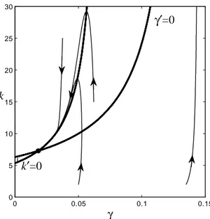
The local asymptotic stability of the dynamic equilibrium ( ; k ) relies on the condition det J ( ; k ) > 0 and tr J ( ; k ) < 0. Such condition is ful…lled, provided that the adjustment parameter is su¢ ciently close to zero. Stability is strictly local and, as shown in Fig. 1, for initial conditions outside the basin of attraction of ( , k ), trajectories diverge to in…nity.

In the parameter range in which local stability obtains, it is meaningful to consider the persistent e¤ects of a change in distribution. Since long-term growth is exogenous, the pro…t share does not have steady-growth e¤ects, but only level e¤ects. A lower pro…t share causes higher productivity adjusted output y and capital stock k , hence higher steady-state employment.

It may be worth stressing that the qualitative dynamic properties of sys-tem (17)-(18) are in many respects similar to those of other demand-led growth models in which the engine of growth is provided by autonomous ex-penditure (Allain, 2015; Freitas and Serrano, 2015; Lavoie, 2016). The only, but somewhat crucial di¤erence, is that in the present framework labour pro-ductivity is growing and, provided that the real wage is growing in line with productivity, labour employment would be constant on the steady-growth

3_{The Jacobian matrix of system (17)-(18) evaluated at (0; 0) = (0; 0) is:}

(0; 0) 0 0 (0; 0)

The dynamic instability of the trivial stationary state follows from the fact that (0; 0) > 0.

0 0.05 0.1 0.15 0 5 10 15 20 25 30 γ′=0 k′=0 γ k

Figure 1: Trajectories in phase space for parameter settings pz = 1, = 0:05,

gT = 0:04, u = 0:10, = 0:75, = 0:3, = 0:03, un = 0:775, v = 1:3,

rA = 0:55 such that 0:0184 and k 7:2846. The trajectory on the

right is diverging

path, while average employment would be mildly rising or falling on the transition path, depending on whether ut happened to be lower or higher

than un, at the initial date t = 0.

The scenario of rising labour productivity …ts well with the assumption that output is never constrained by labour supply, but topics for debate are the plausibility of a rising real wage in the face of a steady level of employment, and the motivation behind the assumed R&D expenditure by …rms. The second issue, together with the relation between the pro…t share and the rate of growth, is addressed in the next section.

4

Endogenous technological progress

In this section it is assumed that R&D activity is carried out by an inde-pendent …rm, to the end of selling updating tool-kits to …rms producing consumption and investment goods. A tool-kit is an intermediate good4

pro-duced with one unit of output and the routine embodied in it. The updating tool-kit has unit price pz > 1 that comes from the intellectual property

rights on the routine.5 _{We shall abstract from free entry in R&D, for the}

sake of simplicity. With …rms’ updating expenditure Zt speci…ed as in (7)

above, the pro…t from selling the updating tool-kits, net of the production and R&D cost, is

R;t= (pz 1) KtgT 1

1 1 + rA

Rt (21)

For any given kt = Kt=At…xed by past history, the maximization of pro…t R;t, with respect to Rt, yields the productivity adjusted R&D expenditure

as a function of kt

rA(kt) =

0 if kt kmin

[gT(pz 1) k]1=2 1 if kt> kmin

(22) where kmin = [gT(pz 1) ] 1 > 0. In the range k > kmin, rA(k) is an

increasing function of k; more precisely, r0_A(kt) = 0 if 0 < kt kmin 1 2[gT(pz 1) ] 1=2_k 1=2 t if kt> kmin (23) Endogenous productivity growth is

_ At At = gT 1 1 1 + rA(kt) (24) The ratios Rt=Kt and Zt=Kt are:

rt = rA(kt)kt1 (25)

zt = pz gT 1

1 1 + rA(kt)

(26) In this section we introduce a ‡ow of autonomous consumption expendi-ture Et that is in‡uenced by the productivity level in the economy, according

to Et = eAt. The term e = Et=At is labelled ‘productivity adjusted

au-tonomous consumption’and we assume e > 1. As before, market clearing in the good market requires

Yt = Zt+ Rt+ Ct+ It+ Et (27)

5_{The assumption that the price p}

z is …xed and greater than one is justi…ed by the

hypothesis that monopoly price is constrained by the potential entry of imitators, who can produce the tool-kit at a constant unit cost pz> 1. See Aghion and Howitt (2009).

whereas the short-term-equilibrium rate of capacity utilization is now: ut=

v(zt+ rt+ + t+ ekt1 uun)

t v u

(28) By substituting for ut in (12), and taking into account that rA= rA(kt), the

growth rate of the capital stock is

gK;t= t+ F ( t; kt), (29) where F ( t; kt) is de…ned by F ( _t; kt) = x pz gT 1 1 1 + rA(kt) +rA(kt) kt + + e kt + _t un v (30) The Harrodian adjustment rule (17) for long-term expectations _t can now be expressed in compact form as

__t= F ( _t; kt) t (31)

while using (24) the law of motion (18) for kt becomes:

_kt = t+ F ( t; kt) gT 1

1 1 + rA(kt)

kt (32)

As in the previous section, we have a dynamic system in the two state variables _t and kt such that its dynamic equilibria satisfy _t = _kt = 0.

One equilibrium is the positive steady state ( ; k ), where = (k ) = gT [1 (1 + rA(k )) 1]and k is the positive real solution to F ( (k ); k ) =

0. The properties of the dynamic equilibrium ( ; k ) are discussed below. To this end, let

h g_T1=2 (1 + pz )[(pz 1) ] 1=2 [(pz 1) ]1=2 > 0 (33)

s un=v gT(1 + pz ) 0 (34)

Notice that conditions (33) and (34) rely upon the plausible parameter re-strictions pz 1 < (1 + )= and = ( + gT(1 + ))v=un: Appendix

A:1 shows that, with such restrictions in place, we have:

k = 2(e 1) h + 1=2 2 (35) where = h2+ 4(e 1)s.

Thus, a necessary condition for the existence of a positive growth path is that productivity adjusted autonomous consumption e is larger than one. It may be also worth observing that k is negatively related to the value of the pro…t share, and because is an increasing function of k , we say that growth is wage led in the equilibrium ( ; k ).6

To study the local stability of ( ; k ), we write the Jacobian matrix of the …rst partial derivatives of system (31)-(32), evaluated at ( ; k ), i.e.:

J ( ; k ) = x Fk( ; k ) (1 + x)k k Fk( ; k ) 1₂g 1=2 T [(pz 1) k ] 1=2 This yields: det(J ( ; k )) = k Fk( ; k ) + x 1 2 gT k 1=2 [(pz 1) ] 1=2 tr(J ( ; k )) = x + k Fk( ; k ) 1 2 gT k 1=2 [(pz 1) ] 1=2

If technological opportunity gT is small enough, then sign[det(J ( ; k ))] =

sign[Fk( ; k )], and if the adjustment parameter is su¢ ciently small,

then tr(J ( ; k )) < 0, if Fk( ; k ) < 0. It turns out that the local

stabil-ity of the constant growth path ( ; k )hinges crucially upon the condition Fk( ; k ) < 0. Appendix A:2 shows that this restriction applies, thus

yield-ing:

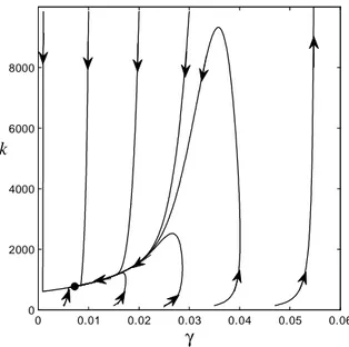
Proposition 1 If e > 1, in the range of the pro…t share , there ex-ists a positive steady state solution ( ; k ) of the dynamic system (31)-(32). ( ; k ) is locally asymptotically stable, if technological opportunity gT and

the adjustment parameter are small enough. An illustration of this case is shown in Fig. 2.

4.1

Comparative analysis

The transitional and steady state e¤ects of a change in distribution on both output and employment are worth considering. In the parameter range in which the local stability of the positive dynamic equilibrium holds, let us contemplate an economy that at time t is fully adjusted to its steady-state position ( 1; k1), corresponding to = 1. Labor productivity is At and

capacity utilization is ut = un; thus, we can write AtLt = unKt and Lt =

6_{This borrows a terminology …rst introduced in Rowthorn (1982), Dutt (1984), Bhaduri}

0 0.01 0.02 0.03 0.04 0.05 0.06 0 2000 4000 6000 8000 γ k

Figure 2: Trajectories in phase space for parameter settings: = 0:3, gT =

0:04, = 0:15, v = 3, = 0:08, pz = 1:6, = 0:02, e = 40, un = 0:8, u = 0:025 such that 0:0072 and k 775:6656 The trajectory on the

right is diverging

L1 = unk1. At time t + @t a once and for all small parametric change

of the pro…t share takes place, such that = 2 1 > 0. Because

k is a decreasing function of , after convergence to the new steady state ( ₂; k₂), corresponding to 2, productivity adjusted output is y2 < y1. The

new steady-state level of employment is L2 = unk2 < L1. Thus, a once

and for all rise of the pro…t share causes a persistent fall in steady-state employment. In the new steady state, output grows at the lower rate ₂ <

1. Conversely, a fall < 0 of the pro…t share would cause a persistent

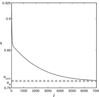
increase of the growth rate and a persistent rise in employment, but no persistent e¤ect on the rate of capacity utilization, that will eventually return to its steady-state normal level un. Still, as shown in Fig. 3, over any …nite

time interval, following the given fall of the pro…t share, average capacity utilization is higher than normal. This marks a sharp distinction between the time average of a variable, over a long interval of historical time, and its dynamic attractor.7

7_{Debates over the role and properties of capacity utilization in the analysis of}

0 1000 2000 3000 4000 5000 6000 7000 0.79 0.85 0.9 0.925 u_n u_ave t u

Figure 3: Behaviour in time of the rate of capacity utilization after an exoge-nous, once and for all change of the pro…t share = 0:03, with all other parameters as in Fig. 2 and initial condition at the equilibrium ( ; k )

4.2

Limit cycles

Appendix A:3 shows that there are two other equilibria of the dynamic system (31)-(32). One is the unstable trivial solution (0; 0). The other equilibrium is the saddle point (0; k ). The existence of such equilibria derives exclusively from the multiplicative terms t and kt, that appear on the right-hand of

(31) and of (32), respectively. Still, the grounds for introducing such terms are not the same. The multiplicative term kt in the right-hand side of (32) is

imposed by formal and logical consistency, including the necessary restriction kt 0. On the contrary, the multiplicative term t in the right-hand side

of (31) cannot be justi…ed on similar grounds. While the form (31) requires

t 0, such non-negativity restriction, far from being a logical requirement,

is objectionable outside a strictly-local domain of analysis.

In our attempt to proceed in this direction, we eliminate the multiplica-tive term t in (31) and, borrowing insights from the non-linear adjustment

literature (Goodwin, 1951), we further impose that as the gap between the long-term expectation _t and the ex-post observation gK;t tends to increase,

the adjustment rule of t becomes increasingly conservative. Thus, using

(29) we replace (31) with:

-0.02 -0.01 0 0.01 0.02 400 600 800 1000 1200

(a)

γ

k

(b)

γ

k

Figure 4: (a) Convergence to the external limit cycle in phase space for parameter settings = 0:3, gT = 0:035, 0:1031, v = 3, = 0:08,

pz = 1:6, = 0:02, e = 40, un = 0:8, u = 0:025, = 660 and initial

conditions ( 01; k01) = (0; 565), ( 02; k02) = (0; 1100) ; (b) coexistence of two

limit cycles

As it can be readily observed, the two equilibria (0; 0) and (0; k ) vanish, but the equilibrium ( ; k )does not. Appendix A.4 proves that the local stability properties of the equilibrium ( ; k ) are qualitatively unchanged: namely, there exists a value ^ > 0, such that ( ; k ) is locally asymptotically stable if 0 < < ^. In this parameter range of , the temporary and persistent qualitative e¤ects of a small change in distribution are those described in paragraph 4.1. For any > ^ the dynamic equilibrium ( ; k ) is unstable, and growth trajectories with initial conditions in a neighbourhood of the steady state, converge to a limit cycle around ( ; k ). This is proved as follows (see Appendix A.4).

If = is small enough, there exists a compact positively invariant region D in the state space such that ( ; k ) _{2 D is the unique stationary point} of (36)-(32) in D. In a right-neighbourhood of ^, the equilibrium ( ; k )is unstable, and by the Poincaré-Bendixon theorem, the region D contains a stable limit cycle as shown in Fig. 4(a). In addition, numerical simulation uncovers the existence of a multiplicity of limit cycles around the locally unstable ( ; k )(see, for an example, Fig 4(b)).

The persistent ‡uctuations around the positive steady state are such that the average rate of capacity utilization over the cycles does not coincide with the steady-state normal value un, but is higher (see Fig. 5). This extends the

2000 2020 2040 2060 2080 2100 0.65 0.7 0.75 0.85 0.9 0.95 1 u_n u_ave t u

Figure 5: The cyclical behaviour of the rate of capacity utilization over the external limit cycle of Fig. 4(b)

distinction between the long-term time average of a variable and its dynamic equilibrium to situations in which the economy is on its asymptotic attractor.

5

Conclusions

This paper builds on the hypothesis that R&D and various forms of expen-diture triggered by innovation are autonomous, in that they are relatively una¤ected by short-run output. Moreover, if and to the extent that innova-tions are primarily aimed at reducing the use of the human-labour input in production, while the use of capital inputs per unit of output is …xed, such expenditures do not create new capacity. Thus, they do not interfere with ex-pansion investment, as determined by the state of long-term expectations on output growth and by the wish to bring capacity utilization into line with its desired level. We explore some implications of these hypotheses in the light of a demand-led endogenous-growth model.8 R&D is carried out to maxi-mize monopoly rents and is an increasing function of the capital stock and of the historically given technological opportunities. For the sake of simplicity,

8_{Results of the exogenous-growth framework are skipped for simplicity, because they}

are similar, except for the fact that distribution does not a¤ect the long-run growth of output.

it is assumed that the marginal propensity to save out of wages is one and the marginal propensity to save out of pro…ts is zero. In the short-run equi-librium, the average propensity to save depends on the level of autonomous expenditure. This includes not only R&D and modernization expenditures by …rms, that are both a function of the capital stock. The existence and local stability of the positive growth path requires a ‡ow of autonomous ex-penditure, that grows through time with labour productivity, but bears no strong direct relation with the size of the capital stock.9 _{This ‡ow is here}

interpreted as autonomous consumption …nanced by pro…t income.

The main results are as follows. A su¢ ciently slow adjustment of long term expectations, as parametrized by , ensures the local asymptotic stabil-ity of the positive growth path. At higher values of , the instability of the dynamic equilibrium requires replacing a strictly local expectation-formation rule, with one that may hold on a wider domain. In this case, the growth trajectories starting in a neighbourhood of the dynamic equilibrium remain bounded and converge to limit cycles, provided that the revision of long-term expectations is ever more conservative, as the gap between prediction _t and ex-post realization gK;t increases. On the steady-growth path, capacity

uti-lization is at its desired level. Growth is wage led, both in the sense that long term output growth is inversely related to the pro…t share, and in the sense that a lower pro…t share raises the steady state level of productivity ad-justed output and employment. Employment is constant on a steady-growth path and the output dynamics tends to be divorced from the employment dynamics. A higher pro…t share causing a slower long-run growth of output will in fact produce a persistent fall in employment. In this framework, any fall in the wage share, whether caused by market forces, or by changes in institutions, tends to produce self-reinforcing e¤ects. In this way, the model may contribute to the task of interpreting the association between a falling manufacturing employment and a falling wage share, that are a characteristic of the present era in many western countries.

A

Appendix

A.1

Computation of

k

9_{In the exogenous-growth model in section 3, this expenditure component is identi…ed}

Imposing = gT (1 (1 + rA(k)) 1), the equilibrium restriction F ( ; k) =

0 yields

(1 + pz )gT 1 (1 + rA(k)) 1 + rA(k)k 1+ ek 1 =

un

v Substitute for rA(k) from (22) at k > kmin and rearrange, to obtain

k 1(e 1)+k 1=2g_T1=2[[(pz 1) ]1=2 [(1+pz )[(pz 1) ] 1=2] =

un

v (1+pz )gT that can be written in compact form as

(e 1)y2 hy s = 0

where y = k 1=2 _{and h > 0, s 0are de…ned (respectively) by (33) and (34)}

in the text and by the restrictions spelled out therein. This leads to

y = h +

1=2

2(e 1) where = h2_{+ 4s(e 1) and}

k = 2(e 1)

h + 1=2 2

A.2

Proof that

F

(

; k ) < 0

Using (35) the term 1₂(gTk )1=2 can be written as

1 2(gTk ) 1=2 = e 1 (h=g1=2_T ) + ( =gT) 1=2 (37)

Substituting for h from (33) 1

2(gTk )

1=2

= e 1

(1 + pz )[(pz 1) ] 1=2 [(pz 1) ]1=2+ ( =gT)1=2

Because e > 1 and (pz 1) < 1, we have:

Fk( ; k ) = x (k )2 " (e 1) pz [(pz 1) ] 1=2 [(pz 1) ]1=2 (1 + pz )[(pz 1) ] 1=2 [(pz 1) ]1=2+ ( =gT)1=2 + 1 e # < 0

A.3

Properties of the equilibria

(0; 0) and (

; k )

The Jacobian matrix of the dynamic system (31)-(32) evaluated at (0; 0) is: J (0; 0) = F (0; 0) 0

0 F (0; 0)

and because F (0; 0) > 0, the trivial stationary equilibrium (0; 0) is locally unstable.

Using (31), the equilibrium (0; k ) is de…ned by

F (0; k ) = gT[1 [gT(pz 1) k ] 1=2] (38)

In the interval [0; k ], F (0; k) is a decreasing function of k, that satis…es: F (0; 0) = +_{1, F (0; k}min) > 0 and F (0; k ) < 0. The function (k) de…ned

by (k) gT[1 [gT(pz 1) k ] 1=2] is a non decreasing function of k

and satis…es: (k) = 0 for 0 k kmin; (k) > 0 and 0(k) > 0 at

kmin < k k . By continuity, there exists k > kmin such that condition

(38) holds and F (0; k ) > 0.

The Jacobian matrix of (31), (32) evaluated at (0; k ) is:

J (0; k ) = F (0; k ) 0

(1 + x)k k Fk(0; k ) 1₂g 1=2

T [(pz 1) k ] 1=2

Because F (0; k ) > 0 and Fk(0; k ) < 0, we have det J (0; k ) < 0;

there-fore, (0; k ) is a saddle point.

A.4

Properties of the dynamic system (36)-(32)

The Jacobian matrix of (36)-(32) evaluated at ( ; k )is: ^ J ( ; k ) = x Fk( ; k ) (1 + x)k k Fk( ; k ) 1₂g 1=2 T [(pz 1) k ] 1=2 such that det( ^J ( ; k )) = k Fk( ; k ) + x 1 2 gT k 1=2 [(pz 1) ] 1=2 tr( ^J ( ; k )) = x + k Fk( ; k ) 1 2 gT k 1=2 [(pz 1) ] 1=2

Because Fk( ; k ) < 0(Appendix A.2), there exists ^ > 0, such that ( ; k )

is locally asymptotically stable, if 0 < < ^.

Observe from (30), that if s > 0, there is a …nite k > k , such that for any _{2 [0; g}T], F ( ; k) < 0, if k k > 0 and su¢ ciently small. Moreover,

there is a strictly positive ^k < k , such that, for any _{2 [0; g}T], F ( ; k) > 0,

if k k > 0^ and su¢ ciently small.

Equation (36) implies that _t = 0, if F2( ; k) = = . Moreover,

be-cause F ( ; k) > 0, for each k 2 [^k; k], we can de…ne the correspondence [ ₁(k); ₂(k)]such that F ( ₁(k); k) = ( = )1=2 _{and F (}

2(k); k) = ( = )1=2. Let ^₁(k) = min k2[^k;k] ( ₁(k)); 2(k) = max k2[^k;k] ( ₂(k)).

Notice that ^₁(k) < < ₂(k) and that for = su¢ ciently small we have 0 ^₁(k) < < ₂(k) gT. This proves that there is a positively invariant

region D of (36), (32) around ( ; k ).

References

[1] Allain, O. 2015. Tackling the instability of growth: a Kaleckian-Harrodian model with an autonomous expenditure component, Cam-bridge Journal of Economics, vol. 39, n. 3, 1351-1371

[2] Aghion, P. and Howitt, P. 2009. The Economics of Growth, Cambridge MA, The MIT Press

[3] Bhaduri, A. and Marglin, S.A. 1990. Unemployment and the real wage: the economic basis for contesting political ideologies, Cambridge Journal of Economics, vol. 14, n. 4, 375-393

[4] Cesaratto, S. 2015. Neo-Kaleckian and Sra¢ an controversies on the the-ory of accumulation, Review of Political Economy, vol. 27, n. 2, 154-182 [5] Duesenberry, J.S. 1949. Income, Saving and the Theory of Consumer

Behavior, Cambridge MA, Harvard University Press

[6] Dutt, A.K. 1984. Stagnation, income distribution, and monopoly power, Cambridge Journal of Economics, vol. 8, n. 1, 25-40

[7] Falk, M. 2006. What drives business Research and Development (R&D) intensity across Organisation for Economic Co-operation and Develop-ment (OECD) countries?, Applied Economics, vol. 38, n. 5, 533-547

[8] Freitas, F. and Serrano, F. 2015. Growth rates and level e¤ects, the stability of the adjustment of demand to capacity, and the Sra¢ an su-permultiplier, Review of Political Economy, vol. 27, n. 3, 258-281 [9] Girardi, D. and Pariboni, R. 2015. Autonomous demand and economic

growth: some empirical evidence, Working Paper 714, Dipartimento di Economia Politica e Statistica, University of Siena

[10] Goodwin, R.M. 1951. The nonlinear accelerator and the persistence of business cycles, Econometrica, vol. 19, n. 1, 1-17

[11] Harho¤, D. 1998. Are there …nancing constraints for R&D and invest-ment in German manufacturing …rms?, Annales d’Économie et de Sta-tistique, n. 49/50, 421–56

[12] Hicks, J.R. 1950. A Contribution to the Theory of the Trade Cycle, Ox-ford, The Clarendon Press

[13] Keynes, J.M. 1973. Ex-post and ex-ante, 1937 lecture notes; reprinted in The Collected Writings of John Maynard Keynes, vol 14, London, Macmillan for the Royal Economic Society, pp. 179-183

[14] Lavoie, M. 2016. Convergence towards the normal rate of capacity uti-lization in neo-Kaleckian models: the role of non-capacity creating au-tonomous expenditures, Metroeconomica, vol. 67, n. 1, 172-201

[15] Lavoie, M. 2017. Prototypes, reality and the growth rate of autonomous consumption expenditures: a rejoinder, Metroeconomica, vol. 68, n. 1, 194-199

[16] Marglin, S.A. and Bhaduri, A. 1990. Pro…t squeeze and Keynesian the-ory, in S.A. Marglin and J.B. Schor (eds), The Golden Age of Capitalism: Reinterpreting the Postwar Experience, Oxford, The Clarendon Press, pp. 153–186

[17] Rezai, A. 2012. Goodwin cycles, distributional con‡ict, and productivity growth, Metroeconomica, vol. 63, n. 1, 29-39

[18] Rowthorn, R.E. 1982. Demand, real wages and economic growth, Studi Economici, vol. 18, 2-53

[19] Serrano, F. 1995A. Long-period e¤ective demand, and the Sra¢ an su-permultiplier, Contributions to Political Economy, vol. 14, 67-90

[20] Serrano, F. 1995B. The Sra¢ an Supermultiplier. Unpublished Phd The-sis, University of Cambridge, UK

[21] Serrano, F. and Freitas, F. 2017. The Sra¢ an supermultiplier as an alternative closure for heterodox growth theory, in European Journal of Economics and Economic Policies, vol. 14, 70-91

[22] Setter…eld, M. 2016. Wage- versus pro…t- led growth after 25 years: an introduction, Review of Keynesian Economics, vol. 4, 367-372

[23] Trezzini, A. 2017. Harrodian instability: a misleading concept, Centro Sra¤a, Working Papers n. 24

[24] Trezzini A. and Palumbo, A. 2016, The theory of output in the modern classical approach: main principles and controversial issues, Review of Keynesian Economics, vol. 4, 503-522