The Bipolar Choquet Integral Representation
Fabio Rindone
Faculty of Economics
Contents
Preface 7
1 Historical Background 13
1.1 The St. Petersburg paradox . . . 13
1.2 von Neumann and Morgenstern . . . 15
1.3 Descriptive Limitations of Expected Utility Theory . . . 21
1.3.1 Allais paradoxes . . . 21
1.3.2 The early evidence . . . 23
1.4 The Axioms for Subjective Probability . . . 28
1.4.1 Introduction . . . 28
1.4.2 De Finetti’s axioms . . . 29
1.5 Savage’s Theorem . . . 32
1.5.1 States, outcomes, and acts . . . 32
1.5.2 Axioms . . . 35
1.5.3 The theorem . . . 41
1.6 A critique of Savage . . . 43
1.6.1 Critique of P3 and P4 . . . 43
1.6.3 Ellsberg’s urns . . . 45
1.7 Concluding remarks . . . 48
2 Bipolar Cumulative Prospect Theory 51 2.1 Introduction . . . 51
2.2 Cumulative Prospect Theory . . . 55
2.2.1 CPT fundamental concepts . . . 55
2.2.2 The formal model . . . 57
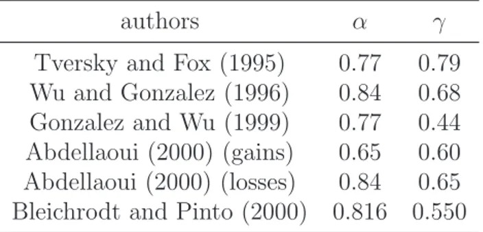
2.2.3 CPT parametrization . . . 60
2.3 Bipolar Cumulative Prospect Theory . . . 60
2.3.1 From CPT to bCPT . . . 60
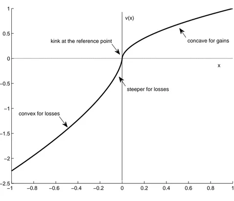
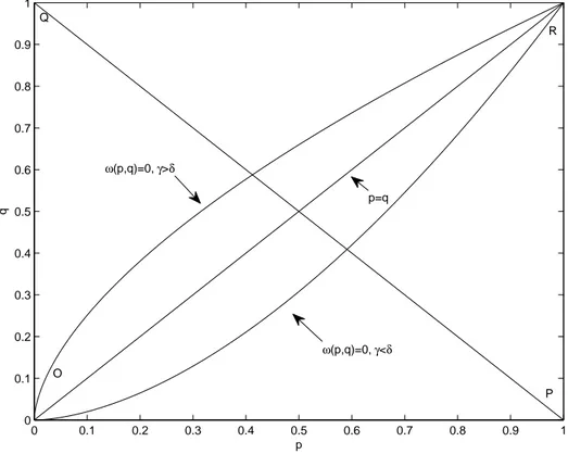
2.3.2 The bi-weighting functions . . . 62
2.3.3 The bipolar Cumulative Prospect Theory (bCPT) . . . 66
2.3.4 bCPT and Stochastic Dominance . . . 67
2.3.5 The relationship between CPT and bCPT . . . 69
2.3.6 Explanation of the Wu-Markle paradox . . . 76
2.4 Appendix . . . 79
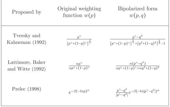
2.4.1 The Kahneman-Tversky bi-weighting function . . . 80
2.4.2 The Latimore, Baker and Witte bi-weighting function . . . 86
2.4.3 The Prelec bi-weighting function . . . 88
3 Explanation of some recent paradoxes against CPT 95
3.1 Recent literature against CPT . . . 95
3.2 Wu and Markle (2008) . . . 96
3.3 Birnbaum-Bahra . . . 100
3.4 Concluding remarks . . . 103
4 The bipolar Choquet Integral 105 4.1 Introduction . . . 105
4.2 Extension of bCPT to uncertainty . . . 106
4.2.1 Bi-capacity and bipolar Choquet integral . . . 106
4.2.2 Two different approaches . . . 108
4.2.3 Link between CPT and bCPT . . . 110
4.3 The characterization theorem . . . 113
4.3.1 Properties and main theorem . . . 113
4.3.2 Continuity and extension to bounded functions . . . . 118
4.3.3 Coherence conditions. . . 121
4.4 Concluding remarks . . . 127
Randomness in Economic
Theory
Surprisingly, risk and uncertainty have a rather short history in eco-nomics. The formal incorporation of these concepts into economic theory was only accomplished when Von Neumann and Morgenstern (1944) pub-lished their Theory of Games and Economic Behavior - although the excep-tional effort of Ramsey (1926) and Keynes (1921) must be mentioned as an antecedent. Indeed, the very idea that risk and uncertainty might be rele-vant for economic analysis was only really suggested by Frank Knight (1921) in his formidable treatise, Risk, Uncertainty and Profit. What makes this lateness even more surprising is that the very concept of marginal utility, the foundation stone of Neoclassical economics, was introduced by Bernoulli (1738)1
in the context of choice under risk. Bernoulli’s notion of expected utility which decomposed the valuation of a risky venture as the sum of util-ities from outcomes weighted by the probabilutil-ities of outcomes, was generally not appealed to by economists. Part of the problem was that it did not seem sensible for rational agents to maximize expected utility and not
some-1
thing else. Specifically, Bernoulli’s assumption of diminishing marginal utility seemed to imply that, in a gamble, a gain would increase utility less than a decline would reduce it. Consequently, many concluded, the willingness to take on risk must be “irrational”, and thus the issue of choice under risk or uncertainty was viewed suspiciously, or at least considered to be outside the realm of an economic theory which assumed rational actors. The great task of Von Neumann and Morgenstern (1944) was to lay a rational foundation for decision-making under risk according to expected utility rules. However the novelty of using the axiomatic method - combining sparse explanation with often obtuse axioms - ensured that most economists of the time would find their contribution inaccessible. Restatements and re-axiomatizations by Marschak (1950); Samuelson (1952); Herstein and Milnor (1953) did much to improve the situation. A second revolution occurred soon afterwards. The expected utility hypothesis was given a celebrated subjectivist twist by Sav-age (1954) in his classic Foundations of Statistics. Inspired by the work of Ramsey (1926) and De Finetti (1931, 1937), Savage derived the expected utility hypothesis without imposing objective probabilities but rather by al-lowing subjective probabilities to be determined jointly. Savage’s brilliant performance was followed up by Anscombe and Aumann (1963). In some re-gards, the Savage-Anscome-Aumann subjective approach to expected utility has been considered more general than the older von Neumann-Morgenstern concept. Another “subjectivist” revolution was initiated with the “state-preference” approach to uncertainty of Arrow (1964) and Debreu (1959). Although not necessarily opposed to the expected utility hypothesis, the state-preference approach does not involve the assignment of mathematical
probabilities, whether objective or subjective, although it often might be use-ful to do so. The structure of the state-preference approach is more amenable to Walrasian general equilibrium theory where payoffs are not merely money amounts but actual bundles of goods. In economic theory, utility is usually understood as a numerical representation of a preference relation; preferences are assumed to satisfy certain condition of internal consistency, axioms, which ensure that a utility representation exists for preferences and that choosing consistently with one’s preferences can be represented as the maximization of utility. Expected utility theory imposes a particular set of consistency conditions, which imply that choice under uncertainty can be represented as the maximization of the mathematical expectation of the utility of conse-quences. Famous paradoxes such as those in Shackle (1952); Allais (1953); Ellsberg (1961), have been presented to critic this set of axioms underling the expected utility theory, see Camerer (1995) for an overview. On the other hand, influential experimental studies, such as those by Kahneman and Tversky (1979), have revealed a range of systematic patterns of behav-ior which appear to contravene expected utility theory. These motivations reinforced the need to rethink and to re-axiomatize much of the theory of choice under risk and uncertainty. In the last thirty years, an enormous amount of work has been done to develop new decision theories, the so called
non-expected utility theories, which can accommodate at least some of the
patterns of choice that contravene expected utility theory. Non expected utility theories impose different - usually weaker - consistency conditions with respect to those imposed by utility theory, which represent choice un-der uncertainty as the maximization of some other function rather than the
mathematical expectation of the utility of consequences. Over these alter-native theories, are worthy to be mentioned: weighted expected utility (e.g. Allais and Hagen (1979); Chew and MacCrimmon (1979); Fishburn (1983)), rank-dependent expected utility (Quiggin (1982); Yaari (1987)), non-linear expected utility (e.g. Machina (1982)), regret theory (Loomes and Sugden (1982), non-additive expected utility (Shackle (1949); Schmeidler (1989)) and state-dependent preferences (Karni (1985)). Prospect Theory (PT) of Kah-neman and Tversky (1979) merits a special mention. Due to the great de-scriptive powerful of the theory, the two authors (psychologists) imposed initially prospect theory as a descriptive model, without an axiomatic foun-dation. The modern version Cumulative Prospect Theory (CPT), Tversky and Kahneman (1992), is nowadays considered one of the most suitable gen-eralization of classical expected utility. With CPT the authors generalized PT, and summarized the most relevant ideas contained in the other non-expected utility theories. Since CPT is nowadays considered the reference model of choice under risk and uncertainty, most of empirical studies are designed to test it. In very recent years some critiques have been advanced against CPT, particularly regarding the gain loss separability, i.e. the fact that in the model gains and losses contained within a lottery are evaluated separately, and then summed to obtain an overall evaluation. These critiques have been formalized in many studies, the most relevant of which is surely Wu and Markle (2008). With this thesis we aim to generalize CPT, allowing gains and losses within a mixed prospect to be evaluated conjointly, in this bypassing the critique regarding the gain loss separability but retaining the main features of CPT. We call our model the bipolar Cumulative Prospect
Theory (bCPT), to underline that we retain it the most natural extension of CPT. At the end we wish to point out that this thesis does not provide a full preference foundation of bCPT, i.e. the model is not elicited from a set of axioms, but we use an utility-based method. We think most theorist of choice under uncertainty will acknowledge that, in their actual practice, they use axiomatic and utility-based methods in parallel. Some new theories have been developed out of the consideration of alternative axioms about prefer-ences, but in many cases, theories were initially developed in the language of utility and the equivalent axiomatic form were discovered later. Expected utility theory itself provides an extreme example of this process: the utility-based form of this theory preceded its axiomatic form by about two hundred years. In recent years PT (utility-based) preceded CPT by thirteen years. It is not obvious, then, that the axiom-based versions of theories are more fundamental than the utility-based versions.
Chapter 1
Historical Background
1.1
The St. Petersburg paradox
During the development of probability theory in the 17th century, math-ematicians such as Blaise Pascal and Pierre de Fermat assumed that the attractiveness of a gamble offering the payoffs (x1, . . . , xn) with probabilities
(p1, . . . , pn) was given by its expected value ∑ixipi.
Nicholas Bernoulli proposed the following St. Petersburg game in 1713, which was resolved independently by his cousin Daniel Bernoulli (in 1738) and Gabriel Cramer (in 1728). Suppose someone offers to toss a fair coin repeat-edly until it comes up heads. If the first head appears at the nth toss, the payoff is $2n−1. What is the largest sure gain you would be willing to forgot
in order to undertake a single play of this game? Typically the gamble is represented as
G = ($20
,2−1; $21
Since its expected value is∑i2−i2i−1= ∑i1/2 = ∞, a person would be willing
to pay any sum to play the game, yet, real-world people is willing to pay only a moderate amount of money. This is the so-called St. Petersburg paradox. Daniel Bernoulli’s solution involved two ideas that have since revolutionized economics: firstly, that people’s utility from wealth, u(w), is not linearly related to wealth w but rather increases at a decreasing rate - the famous idea of diminishing marginal utility; secondly that a person’s evaluation of a risky venture is not the expected return of that venture, but rather the expected utility from that venture.
In general, by Bernoulli’s logic, the valuation of any risky venture takes the expected utility form:
E(u, p, X) = ∑
x∈X
p(x)u(x)
where X is the set of possible outcomes, p(x) is the probability of a particular outcome x∈ X and u ∶ X → R is a utility function over outcomes.
In the St. Petersburg case, the sure gain λ which would yield the same utility as the St. Petersburg gamble, i.e., the certainty equivalent λ of this gamble, is determined by the following equation
u(ω + λ) = 1
2u(ω + 1) + 1
4u(ω + 2) + ⋯
where ω is the person’s initial wealth. For example, when u(x) = ln(x) and ω= $50000, λ is about $9 even thought the gamble has an infinite expected value. Finally we note that as Menger (1934) later pointed out, placing an ironical twist on all this, Bernoulli’s hypothesis of diminishing marginal
utility is actually not enough to solve all St. Petersburg-type Paradoxes. To see this, note that we can always find a sequence of payoffs x1, x2, x3,⋯ which
yield infinite expected value, and then propose, say, that u(xn) = 2n so that
expected utility is also infinite. The Menger game is nowadays called the
super St. Petersburg paradox. Thus, Menger proposed that utility must also
be bounded above for paradoxes of this type to be resolved.
1.2
von Neumann and Morgenstern
While Bernoulli theory - the first statement of EUT - solved the St. Pe-tersburg puzzle, it did not find much favor with modern economists until the 1950s. This is partly explained by the fact that, in the form presented by Bernoulli, the theory presupposes the existence of a cardinal utility scale; an assumption that did not sit well with the drive towards ordinalization during the first half of the twentieth century. Interest in the theory was revived when Von Neumann and Morgenstern (1944) showed that the expected util-ity hypothesis could be derived from a set of apparently appealing axioms on preference. Since then, numerous alternative axiomatizations have been developed, some of which seem highly appealing, some might even say com-pelling, from a normative point of view. To the extent that its axioms can be justified as sound principles of rational choice to which any reasonable person would subscribe, they provide grounds for interpreting EUT norma-tively (as a model of how people ought to choose) and prescripnorma-tively (as a practical aid to choice). Our concern, however, is with how people actually choose, whether or not such choices conform with a priori notions of
ratio-nality. Consequently, we will not be delayed by questions about whether particular axioms can or cannot be defended as sound principles of rational choice, and I will start from the presumption that evidence relating to actual behavior should not be discounted purely on the basis that it falls foul of conventional axioms of choice.
In the von Neumann-Morgenstern (vNM) hypothesis, probabilities are as-sumed to be “objective” or exogenously given by “Nature” and thus cannot be influenced by the agent. The problem of an agent under objective uncer-tainty (another name commonly used in the literature is “risk”) is to choose among lotteries. vNM’s original formulation involved decision trees in which compound lotteries were explicitly modeled. We use here the more compact formulation of Fishburn (1970), which implicitly assumes that compound lotteries are simplified according to Bayes’s formula. Thus, lotteries are de-fined by their distributions, and the notion of “mixture” implicitly supposes that the decision maker is quite sophisticated in terms of her probability calculations. Let X be a set of alternatives. There is no additional struc-ture imposed on it. X can be a familiar topological and linear space, but it can also be anything you wish. In particular, X need not be restricted to a space of product-bundles such as Rl
+ and it may include outcomes such as,
God forbid, death. The objects of choice are lotteries with finite support. Formally, define
L = {P ∶ X → [0, 1] ∣ # {x ∣ P(x) > 0} < ∞ ∧ ∑
x∈X
Observe that the expression∑x∈XP(x) = 1 is well-defined thanks to the finite
support condition that precedes it. A mixing operation is performed on L, defined for every P, Q∈ L and every α ∈ [0, 1] as follows: αP + (1 − α)Q ∈ L is given by
(αP + (1 − α)Q)(x) = αP(x) + (1 − α)Q(x)
for every x∈ X. The intuition behind this operation is of conditional prob-abilities: assume that we offer you a compound lottery that will give you the lottery P with probability α and the lottery Q with probability (1 − α). If you know probability theory, you can ask yourself what is the probability to obtain a certain outcome x, and observe that it is, indeed, α times the conditional probability of x if you get P plus (1 − α) times the conditional probability of x is you get Q.
Since the objects of choice are lotteries, the observable choices are modeled by a binary relation,≿, on L, i.e. ≿ ⊆ L × L, where P ≿ Q means that lottery P is considered at least as “good” as lottery Q and the strict preference ≻ and indifference ∼ are defined as usually, i.e. ≻ is the asymmetric part of ≿ and ∼ is its symmetric part.
The vNM’s axioms are:
V1. Weak order: ≿ is complete and transitive.
V2. Continuity: For every P, Q, R∈ L if P ≻ Q ≻ R, there exist α, β ∈ (0, 1) such that αP + (1 − α)R ≻ Q ≻ βP + (1 − β)R.
V3. Independence: For every P, Q, R ∈ L and every α ∈ (0, 1), P ≿ Q iff αP+ (1 − α)R ≿ αQ + (1 − α)R.
in consumer theory or in choice under certainty and allows lotteries to be ordered. Continuity may be viewed as a “technical” condition needed for the mathematical representation and for the proof to work. Indeed, one cannot design a real-life experiment in which it could be violated, since its violation would require infinitely many observations. But continuity can be hypothet-ically “tested”by some thought experiments (Gedankenexperiments). For instance, you can imagine very small, but positive probabilities, and try to speculate what your preferences would be between lotteries involving such probabilities. If you are willing to engage in such an exercise, consider the following example, supposedly challenging continuity: assume that P guar-antees $1, Q $0, and R death. You are likely to prefer $1 to nothing, that is, to exhibit preferences P ≻ Q ≻ R. The axiom then demands that, for a high enough α< 1, you will also exhibit the preference
αP + (1 − α)R ≻ Q,
namely, that you will be willing to risk your life with probability (1 − α) in order to gain $1. The point of the example is that you are supposed to say that no matter how small is the probability of death (1 − α), you will not risk your life for a dollar. A counter-argument to this example (suggested by Raiffa) was that we often do indeed take such risks. For instance, suppose that you are about to buy a newspaper, which costs $1. But you see that it is handed free on the other side of the street. Would you cross the street to get it for free? If you answer yes, you are willing to accept a certain risk, albeit very small, of losing your life in order to save one dollar. This
counter-argument can be challenged in several ways. For instance, you may argue that even if you do not cross the street your life is not guaranteed with probability 1. Indeed, a truck driver who falls asleep may hit you anyway. In this case, we are not comparing death with probability 0 to death with probability(1−α, and, the argument goes, it is possible that if you had true certainty on your side of the street, you would have not crossed the street, thereby violating the axiom. In any event, we understand the continuity axiom, and we are willing to accept it as a reasonable assumption for most applications.
The independence axiom is related to dynamic consistency. However, it involves several steps, each of which could be and indeed has been challenged in the literature (see Karni and Schmeidler (1991)). Consider the following four choice situations: 1. You are asked to make a choice between P and Q. 2. Nature will first decide whether, with probability (1 − α), you get R, and then you have no choice to make. Alternatively, with probability α, nature will let you choose between P and Q.
3. The choices are as in (2), but you have to commit to making your choice before you observe Nature’s move.
4. You have to choose between two branches. In one, Nature will first decide whether, with probability(1 − α), you get R, or, with probability α, you get P. The second branch is identical, with Q replacing P .
Clearly, (4) is the choice between αP+(1−α)R and αQ+(1−α)R. To relate the choice in (1) to that in (4), we can use (2) and (3) as intermediary steps, as follows. Compare (1) and (2). In (2), if you are called upon to act, you are choosing between P and Q. At that point R will be a counterfactual
world. Why would it be relevant? Hence, it is argued, you can ignore the possibility that did not happen, R, in your choice, and make your decision in (2) identical to that in (1). The distinction between (2) and (3) has to do only with the timing of your decision. Should you make different choices in these scenarios, you would not be dynamically consistent: it is as if you plan (in (3)) to make a given choice, but then, when you get the chance to make it, you do (or would like to do) something else (in (2)). Observe that when you make a choice in problem (3) you know that this choice is conditional on getting to the decision node. Hence, the additional information you have should not change this conditional choice. Finally, the alleged equivalence between (3) and (4) relies on changing the order of your move (to which you already committed) and Nature’s move. As such, this is an axiom of reduction of compound lotteries, assuming that the order of the draws does not matter, as long as the distributions on outcomes, induced by your choices, are the same. Whether you find the independence axiom compelling or not, we suppose that its meaning if clear. We can finally state the theorem:
Theorem 1 (von Neumann-Morgenstern) The preference relation, ≿,
satisfies axioms V1-V3 if and only if there exists u ∶ X → R such that, for every P, Q∈ L P ≿ Q if and only if ∑ x∈X P(x)u(x) ≥ ∑ x∈X Q(x)u(x)
1.3
Descriptive Limitations of Expected
Util-ity Theory
Empirical studies dating from the early 1950s have revealed a variety of patterns in choice behavior that appear inconsistent with EUT. With hind-sight, it seems that violations of EUT fall under two broad headings: those which have possible explanations in terms of some “conventional” theory of preferences and those which apparently do not. The former category con-sists primarily of a series of observed violations of the independence axiom of EUT; the latter of evidence that seems to challenge the assumption that choices derive from well-defined preferences. Let us begin with the former.
1.3.1
Allais paradoxes
There is now a large body of evidence indicating that actual choice be-havior may systematically violate the independence axiom. Two examples of such phenomena, first discovered by Maurice Allais (1953), have played a particularly important role in stimulating and shaping theoretical devel-opments in non-EU theory. These are the so-called common consequence
effects and common ratio effects. The first sighting of such effect came in
the form of the following pair of hypothetical choice problems. In the first you have to imagine choosing between the two prospects: P = ($1M, 1) or Q = ($5M, 0.1; $1M, 0.89; 0, 0.01). The first option gives one million of dollars for sure; the second gives five million with a probability of 0.1, one million with a probability of 0.89, otherwise nothing. What would you
choose? Now consider a second problem where you have to choose between the two prospects: P′ = ($1M, 0.11; 0, 0.89) or Q′ = ($5M, 0.1; 0, 0.9).
What would you do if you really faced this choice? Allais believed that EUT was not an adequate characterization of individual risk preferences and he designed these problems as a counterexample. A person with expected util-ity preferences would either choose both “P ” options, or choose both “Q” options across this pair of problems. In fact rewriting the prospect P and confronting it with Q
P = ($1M, 0.11; $1M, 0.89)
Q= ($5M, 0.1; $1M, 0.89; 0, 0.01).
the preference over P and Q should be independent from the common con-sequence $1M with probability 0.89, so that replacing it with 0 in both the prospects (i.e. P′ and Q′) should not reverse the preference. Allais expected
that people faced with these choices might opt for P in the first problem, lured by the certainty of becoming a millionaire, and select Q′ in the
sec-ond choice where the odds of winning seem very similar, but the prizes very different. Evidence quickly emerged that many people did respond to these problems as Allais had predicted. This is the famous “Allais paradox” and it is one example of the more general common consequence effect. Allais was the first who discovered this phenomenon, however, numerous studies have found that choices between prospects with this basic structure are systemat-ically influenced by the value of the common consequence. A closely related phenomenon, also discovered by Allais, is the so-called common ratio effect.
Suppose you had to make a choice between $3000 for sure, or entering a gam-ble with an 80 percent chance of getting $4000 (otherwise nothing). What would you choose? Now think about what you would do if you had to choose either a 25 percent chance of gaining $3000 or a 20 percent chance of gaining $4000. A good deal of evidence suggests that many people would opt for the certainty of $3000 in the first choice and opt for the 20 percent chance of $4000 in the second. Such a pattern of choice, however, is inconsistent with EUT and would constitute one example of the common ratio effect. More generally, this phenomenon is observed in choices among pairs of problems with the following form: P′′ = (y, p; 0, 1 − p) and Q′′ = (x, λp; 0, 1 − λp)
where x≻ y and λ ∈ (0, 1). Assume that the ratio of “winning”probabilities, λ, is constant, then for pairs of prospects of this structure, EUT implies that preferences should not depend on the value of p. In fact calculating the vNM’s expectation of the two prospects V(P′′) = u(y)p and V (Q′′) = u(x)λp, that
is P′′ ≻ Q′′ iff u(y)p > u(x)λp, i.e. iff u(y)/u(x) > λ, independly by p. Yet
numerous studies (e.g. Loomes and Sugden (1987); Starmer and Sugden (1989)) reveal a tendency for individuals to switch their choice from P′′ to
Q′′ as p falls.
1.3.2
The early evidence
It would, of course, be unrealistic to expect any theory of human behav-ior to predict accurately one hundred percent of the time. Perhaps the most one could reasonably expect is that departures from such a theory is equally probable in each direction. These phenomena, however, involve systematic
(i.e., predictable) directions in majority choice. As evidence against the in-dependence axiom accumulated, it seemed natural to wonder whether its assorted violations might be revealing some underlying feature of preferences that, if properly understood, could form the basis of a unified explanation. Consequently, a wave of theories designed to explain the evidence began to emerge at the end of the 1970s. Most of these theories have the following features in common: (i)preferences are represented by some function V(⋅) defined over individual prospects; (ii) the function satisfies ordering and con-tinuity; and (iii) while V(⋅) is designed to permit observed violations of the independence axiom, the principle of monotonicity is retained. We will call theories with these properties conventional theories. The general spirit of the approach is to seek “well behaved” theories of preference consistent with observed violations of independence; this general approach can be called the
conventional strategy. There is evidence to suggest that failures of EUT may
run deeper than violations of independence. Two assumptions implicit in any conventional theory are: procedure invariance, i.e. preferences over prospects are independent of the method used to elicit them; and description
invari-ance, i.e. preferences over prospects are purely a function of the probability
distributions of consequences implied by prospects and do not depend on how those given distributions are described. While these assumptions probably seem natural to most economists, so natural that they are rarely even dis-cussed when stating formal theories, there is ample evidence that, in practice, both assumptions fail. One well-known phenomenon, often interpreted as a failure of procedure invariance, is preference reversal. The classic preference reversal experiment requires individuals to carry out two distinct tasks
(usu-ally separated by some other intervening tasks). The first task requires the subject to choose between two prospects: one prospect (often called the $-bet) offers a small chance of winning a “good” prize; the other (the “P -bet”) offers a larger chance of winning a smaller prize. The second task requires the subject to assign monetary value - usually minimum selling prices denoted M($) and M(P) - to the two prospects. Repeated studies (Tversky and Thaler (1990); Hausman (1992); Tammi (1997)) have revealed a tendency for individuals to chose the P -bet (i.e., reveal P ≻ $) while placing a higher value on the $-bet (i.e., M($) > M(P)). This is the so-called preference
reversal phenomenon first observed by psychologists Lichtenstein and Slovic
(1971); Lindman (1971). It presents a puzzle for economics because, viewed from the standard theoretical perspective, both tasks constitute ways of ask-ing essentially the same question, that is, “which of these two prospects do you prefer?” In these experiments, however, the ordering revealed appears to depend upon the elicitation procedure. One explanation for preference reversal suggests that choice and valuation tasks may invoke different men-tal processes which in turn generate different orderings of a given pair of prospects (see Slovic et al. (1995)). Consequently, the rankings observed in choice and valuation tasks cannot be explained with reference to a single preference ordering. An alternative interpretation explains preference rever-sal as a failure of transitivity (see Loomes and Sugden (1983)): assuming that the valuation task reveals true monetary valuations, (i.e., M($) ∼ $; M(P) ∼ P), preference reversal implies P ≻ $ ∼ M($) ≻ M(P) ∼ P; which involves a violation of transitivity (assuming that more money is preferred to less). Although attempts have been made to explain the evidence in ways
which preserve conventional assumptions - see for example Holt (1986); Karni and Safra (1987); Segal (1988) - the weight of evidence suggests that failures of transitivity and procedure invariance both contribute to the phenomenon (Loomes et al. (1989); Tversky et al. (1990)). There is also widespread evi-dence that very minor changes in the presentation or “framing” of prospects can have dramatic impacts upon the choices of decision makers: such effects are failures of description invariance. Here is one famous example due to Tversky and Kahneman (1981) in which two groups of subjects-call them groups I and II-were presented with the following cover story: “Imagine that
the U.S. is preparing for the outbreak of an unusual Asian disease, which is expected to kill 600 people. Two alternative programs to combat the disease have been proposed. Assume that the exact scientific estimate of the conse-quences of the programs are as follows:...” Each group then faced a choice
between two policy options. Options presented to group I: “If program A is
adopted, 200 people will be saved. If program B is adopted, there is a 1/3 probability that 600 people will be saved, and a 2/3 probability that no people will be saved.” Options presented to group II: “If program C is adopted, 400 people will die. If program D is adopted, there is a 1/3 probability that nobody will die, and a 2/3 probability that 600 people will die.”
The two pairs of options are stochastically equivalent. The only difference is that the group I description presents the information in terms of lives saved while the information presented to group II is in terms of lives lost. Tversky and Kahneman found a very striking difference in responses to these two presentations: 72 percent of subjects preferred option A to option B while only 22 percent of subjects preferred C to D. Similar patterns of response
were found amongst groups of undergraduate students, university faculty, and practicing physicians. Failures of procedure invariance and description invariance appear, on the face of it, to challenge the very idea that choices can, in general, be represented by any well behaved preference function. If that is right, they lie outside the explanatory scope of the conventional strategy. Some might even be tempted to say they lie outside the scope of economic theory altogether. That stronger claim, however, is controversial, and we will not be content to put away such challenging evidence so swiftly. For present purposes, suffice it to make two observations. First, whether or not we have adequate economic theories of such phenomenon, the “Asian disease“ example is clearly suggestive that framing effects have a bearing on issues of genuine economic relevance. Second, there are at least some theories of choice that predict phenomena like preference reversal and framing effects, and some of these models have been widely discussed in the economics lit-erature. Although most of these theories draw on ideas about preference to explain choices, they do so in unorthodox ways, and many draw on concepts more familiar to psychologists than economists. The one feature common to this otherwise heterodox bunch of theories is that none of them can be reduced to, or expressed purely in terms of, a single preference function V(⋅) defined over individual prospects. We will call such models non-conventional
1.4
The Axioms for Subjective Probability
1.4.1
Introduction
As we have seen in the vNM’s approach the probabilities are objective. First to describe the model of Subjective Expected Utility of Savage (1954) we need some preliminaries about the concept of subjective probability. The most influential contributes on this field are due to Ramsey (1926); De Finetti (1931, 1937); Savage (1954).
The axioms of subjective probability refer to assumed properties of a binary relation “is more probable than”, on a set of propositions or events. This relation often referred to as a qualitative or comparative probability relation, can be taken either as an undefined primitive (intuitive views, Koopman and Good) or as a relation derived from a preference relation (decision-oriented approach, Ramsey, de Finetti and Savage).
Definition 1 Let S be a non-empty set. A Boolean algebraA for S is a
non-empty collection of subsets of S such that it is closed under complementation and finite unions.
A probability measure µ on A satisfies: (a) µ(X) ≥ 0 for all X ∈ A;
(b) µ(X ∪ Y ) = µ(X) + µ(Y ) whenever X and Y are disjoint elements in A; (c) µ(S) = 1.
Definition 2 A σ−Algebra A for S is a Boolean Algebra which satisfies
Xi∈ A for i = 1, 2, ⋯ ⇒ ∞
⋃
i=1
Definition 3 A probability measure µ on a σ−Algebra A is countable
addi-tive (or σ-addiaddi-tive) if
µ( ∞ ⋃ i=1 Xi) = ∞ ∑ i=1 µ(Xi)
whenever Xi∈ A for i = 1, 2, ⋯ and Xi∩ Xj = ∅ for i ≠ j.
1.4.2
De Finetti’s axioms
Let S be the set of states and A be an algebra of subsets of S.. We refer to each A ∈ A as an event. We take the binary relation ≿ on A as basic. Read A≿ B as “event A is at least as probable as event B.”. As usually the asymmetric part of this relation is denoted with ≻ and the symmetric part with ∼; so we will read A ≻ B as “event A is more probable than event B” and A∼ B as “event A and B are equiprobable”.
Definition 4 A probability measure p on A agrees with ≿ if for all A, B ∈ A
A≿ B iff p(A) ≥ p(B) (1.2)
Savage (1954) defines ≿ as a qualitative probability when it satisfies the following axioms proposed by de Finetti, which are clearly necessary con-dition on ≿ for there to be a representation by a probability measure as in (1.2).
• (S1) weak order: ≿ on A is a weak order, i.e it is complete and transitive; • (S2) non-triviality: S ≻ ∅;
• (S4) additivity or independence: If A− C = ∅ = B − C, then A ≻ B iff A∪ C ≻ B ∪ C;
The question of whether de Finetti’s axioms, (S1)-(S4) are sufficient for agreement remained open until it was settled in the negative by Kraft et al. (1959). In the following we assume thatA is finite. Without loss of generality, let A be the family of all subsets of S = {1, 2, ⋯, n}, that is A = 2S. For
convenience, let pi= p(i), i = 1, ⋯, n. Then p agrees with ≿, if for all A, B ∈ A:
A≿ B ⇔ ∑
i∈A
pi ≥ ∑ i∈B
pi (1.3)
Example (Kraft et al. (1959)). Let n= 5, with the following comparisons.
{1, 3, 4} ≻ {2, 5} ≻ {1, 2, 4} ≻ {1, 5} ≻ {3, 4} ≻ {2, 4} ≻ {1, 2, 3} ≻ {5} ≻ {2, 3} ≻ {1, 4} ≻ {4} ≻ {1, 3} ≻ {1, 2} ≻ {3} ≻ {2} ≻ {1} ≻ ∅.
The rest of≻ is given by complementarity ( A ≻ B ⇔ Bc Ac ) and additivity,
hence {4} ≻ {1, 3}, {2, 3} ≻ {1, 4}, {1, 5} ≻ {3, 4}, {1, 3, 4} ≻ {2, 5}. If (1.3) holds, then p4> p1+ p3, p2+ p3 > p1+ p4,
p1+ p5> p3+ p4,
p1+ p3+ p4 > p2+ p5.
Addition and cancellation leave us 0> 0, a contradiction.
Let(A1, . . . , Am) =0 (B1, . . . , Bm) mean that the Aj and Bj are in A and,
for each i= 1, . . . , n the number of Aj that contain i equals the number of Bj
that contain i. In other words, the sums of the indicator functions over the two event sequences are identical. Clearly, for any real numbers p1. . . pn, we
have (A1, . . . , Am) =0(B1, . . . , Bm) ⇒ m ∑ j=1i∈A∑j pi = m ∑ j=1i∈B∑j pi
Definition 5 We say that ≿ on A is strongly additive if, for all m ≥ 2 and
all Aj and Bj,
{(A1, . . . , Am) =0(B1, . . . , Bm), Aj ≿ Bj, j< m} → not(Am≻ Bm).
Remark 1 Strong additivity implies weak order as well as additivity. Strong additivity is actually much stronger. Namely, ≿ on A is strongly additive if and only if there are real numbers p1, . . . , pn that satisfy (1.3). In
the special case of subjective probability with pi≥ 0 and ∑ipi = 1, it is enough
to assume that≿ is non-trivial and non-negative as well as strongly additive. This fact is stated by the following theorem which solves the question for finite agreement.
Theorem 2 Suppose that S is non-empty and finite withA = 2S.Then there
is a probability measure p on A for which for all A, B ∈ A:
A≿ B ⇔ ∑
i∈A
pi≥ ∑ i∈B
pi
if and only if (S2) and (S3) hold for ≿ along with strong additivity.
For infinite Algebra we need to add Savage’s Archimedean axiom.
• (S5) A ≻ B implies that there is a finite partition {C1, . . . , Cm} of S
such that A≻ (B ∪ Ci) for i = 1, . . . , m
Theorem 3 Suppose that A = 2S and ≿ on A satisfies (S1) - (S5). Then
there is a unique probability measure p∶ A → [0, 1] such that (a) for all A, B∈ A : A ≿ B iff p(A) ≥ p(B)
(b) for every A∈ A with p(A) > 0 and every 0 < a < 1, there is a B ⊂ A for which p(B) = ap(A).
1.5
Savage’s Theorem
1.5.1
States, outcomes, and acts
The model of Savage (1954) includes two primitive concepts: states and
outcomes. The set of states, S, should be thought as an exhaustive list of
all scenarios that might unfold. A state, in Savage’s words, “resolves all uncertainty”: it should specify the answer to any question you might be interested in. The answer should be deterministic. If, for instance, in a given state an act leads to a toss of a coin, you should further split the state to
two possible states, each consistent with the original one, but also resolving the additional uncertainty about the toss of the coin. The following chapter elaborates on this notion. Observe that Savage considers a one-shot decision problem. If the real problem extends over many period, the decision problem considered should be thought of as a choice of a strategy in a game. The game can be long or even infinite. You think of yourself as choosing a strategy a-priori, and assuming that you will stick to it with no difficulties of dynamic consistency, unforeseen contingencies, and so forth. This is symmetric to the conception of a state as Nature’s strategy in this game. It specifies all the choices that Nature might have to make as the game unfolds. An event is any subset A ⊆ S. There are no measurability constraints, and S is not endowed with an algebra of measurable events. If you wish to be more formal about it, you can define the set of event to be maximal σ−algebra Σ = 2S ,
with respect to which all subsets are measurable. The set of outcomes will be denoted by X. An outcome x is assumed to specify all that is relevant to your well-being, insomuch as it may be relevant to your decision. In this sense, Savage’s model does not differ from utility maximization under certainty (as in consumer theory) or from vNM’s model. In all of these we may obtain rather counter-intuitive results if certain determinants of utility are left outside of the description of the outcomes. The objects of choice are
acts, which are defined as functions from states to outcomes, and denoted by
F. That is,
Choosing an act f , you typically do not know the outcome you will experi-ence. But if you do know both your choice f and the state s, you know that the outcome will be x= f(s). The reason is that a state s should resolve all uncertainty, including what is the outcome of the act f. Acts that do not depend on the state of the world s are constant functions in F. We will abuse notation and denote them by the outcome they result in. Thus, x∈ X is also understood as x∈ F with x(s) = x. There are many confusing things in the world, but this is not one of them. Since the objects of choice are acts, Sav-age assumes a binary relation≿⊆ F × F. The relation will have its symmetric and asymmetric parts, ∼ and ≻ defined as usual. It will also be extended to X with the natural convention. Specifically, for two outcomes x, y ∈ X, we say that x ≿ y if and only if the constant function that yields always x is related by ≿ to the constant function that yields always y. Before we go on, it is worthwhile to note what does not appear in the model. If you’re taking notes, and you know that you’re going to see a theorem resulting in integrals of real-valued functions with respective to probability measures, you might be prepared to leave some space for the mathematical apparatus. You may be ready now for a page of some measure theory, describing the σ-algebra of events. You can leave half a page blank for the details of the linear structure on X, and maybe a few lines for the topology on X. Or maybe a page or so to discuss the topology on F . But none of it is needed. Savage does not assume any such linear, measure-theoretic, or topological structures. If you go back to the beginning of this sub-section, you will find that it says only, There are two sets, S and X, and a relation on S to XS.
1.5.2
Axioms
The axioms are given here in their original names, P1-P7. They do have nicknames, but these are sometimes subject to debate and open to different interpretations. Before to list the axioms, it will be useful to have a bit more notation. As mentioned above, the objects of choice are simply functions from S to X. What operations can we perform on F = XS if we have no
additional structure on X? The operation we used in the statement of (P2) involves “splicing” functions, that is, taking two functions and generating a third one from them, by using one function on a certain sub-domain, and the other on the complement. Formally, for two acts f, g ∈ F and an event A⊆ S, define an act fAg by fAg(s) =⎧⎪⎪⎪⎪⎨⎪⎪⎪ ⎪⎩ g(s) s ∈ A f(s) s ∈ Ac ,
that is, fAg is “f , where on A we replaced it by g.
It is also useful to have a definition that captures the intuitive notion that an event is considered a practical impossibility, roughly, what we mean by a zero-probability event when a probability is given. One natural definition is to say that
Definition 6 an event A is null if, for every f, g ∈ F, with f(s) = g(s) for
all s∈ Ac, then f ∼ g.
That is, if you know that f and g yield the same outcomes if A does not occur, you consider them equivalent. Now we can enunciate the famous seven Savage’s axioms.
P 1 (Ordering) ≿ on F is a weak order, i.e. it is complete and transitive. P 2 (Sure-Thing principle) For every f, g, h, h′∈ F, and every A ⊂ S,
fAhc ≿ gAhc ⇔ fh ′
Ac ≿ gh ′
Ac
P 3 (Eventwise Monotonicity) For every f ∈ F, non-null event A ⊂ S
and x, y∈ X,
x≿ y ⇔ fx A≿ f
y A
P 4 (Comparative Probability) For every A, B⊆ S and for every x, y, z, w∈ X with x ≻ y and z ≻ w,
yx
A≿ yBx ⇔ wzA≿ wzB
P 5 (Non-triviality) There are f, g∈ F such that f ≻ g
P 6 (Small Event Continuity) For every f, g, h ∈ F with f ≻ G, there
exists a partition of S, {A1, A2. . . , An} such that for every i ≤ n,
fAhi≻ g and f ≻ g
h Ai
P 7 (Dominance) Consider acts f, g∈ F and an event A ⊆ S. If it is the
case that, for every s ∈ A, f ≿A g(s), then f ≿A g, and if, for every s ∈ A,
g(s) ≿Af, then g≿Af
In the following we discuss the meaning and some common interpretations of the seven axioms of Savage.
(P1)(Ordering). The basic idea is very familiar, as are the descriptive
and normative justifications. At the same time, completeness is a demand-ing axiom. Observe that all functions in F are assumed to be comparable. Implicitly, this suggests that choices between every pair of such functions can indeed be observed, or at least meaningfully imagined.
(P2)(Sure-Thing Principle). This axiom says that the preference between
two acts, f and g, should only depend on the values of f and g when they differ. Assume that f and g differ only on an event A (or even a subset thereof). That is, if A does not occur, f and g result in the same outcomes exactly. Then, when comparing them, we can focus on this event, A, and ignore Ac. Observe that we do not need to know that f and g are constants
outside of A. Thus, (P2) is akin to requiring that you will have conditional preferences, namely that you have well-defined preferences between f and g conditional on A occurring, and that these conditional preferences determine your choice between f and g if they are equal in case A does not occur. More technically, we can define the conditional preference ≿A as follows
f ≿Ag ⇔ fAhc ≿ gAhc
and we can state that under (P1) and (P2), ≿A is a weak order.
(P3)(Eventwise Monotonicity). Axiom (P3) states, roughly, the
follow-ing. If you take an act, which guarantees an outcome x on an event A, and you change it, on A, from x to another outcome y, the preference between the two acts should follow the preference between the two outcomes x and y (when understood as constant acts). There are two main interpretations
of (P3). One, which appears less demanding, holds that (P3) is simply an axiom of monotonicity. The interpretation of (P3) as monotonicity is quite convincing when the outcomes are monetary payoffs. The other interpreta-tion of (P3), which highlights this issue is the following. The game we play is to try to derive utility and probability from observed behavior. That is, we can think of utility and probability as intentional concepts related to desires and wants on the one hand, and to knowledge and belief on the other. These concepts are measured by observed choices. In particular, if we wish to find out whether the decision maker prefers x to y, we can ask her whether she prefers to get x or y when an event A occurs, i.e., to compare fx
A to f y A. If
she says that she prefers fx
A, we will conclude that she values x more than y.
(P4)(Comparative Probability). This axiom is the counterpart of (P3)
under the second interpretation. Let us continue with the same line of rea-soning. We wish to measure not only the ranking of outcomes, but also of events. Specifically, suppose that we wish to find out whether you think that event A is more likely than event B. Let we take two outcomes x, y such that ≻ y. For example, x will denote $100 and y $0. We now intend to ask you whether you prefer to get the better outcome x if A occurs (and otherwise y), or to get the better outcome if B occurs (again, with y being the alternative). Suppose that you prefer the first, namely, yx
A≿ yxB, then it seems reasonable
to conclude that A is more likely in your eyes than is B. Clearly axioms (P4) avoids contradictory conclusions on this event’s ranking.
(P5)(Non-triviality). If (P5) does not hold, we get f ∼ g for every f, g ∈ F.
This relation is representable by expected utility maximization: you can choose any probability measure and any constant utility function. Moreover,
the utility function will be unique up to a positive linear transformation, which boils down to an additive shift by a constant. But the probability measure will be very far from unique. But since a major goal of the axioma-tization is to define subjective probability, and we want to pinpoint a unique probability measure, which will be “the subjective probability of the deci-sion maker”, P5 appears as an explicit axiom. Not only in the mathematical sense, namely that P5 follows from the representation, but in the sense that
P5 is necessary for the elicitation program to succeed. Someone who is
in-capable of expressing preferences cannot be ascribed subjective probabilities by the reverse engineering program of Ramsey-de Finetti-Savage.
(P6)(Small Event Continuity). This axiom has a flavor of continuity, but
it also has an Archimedean twist. Let us assume that we start with strict preferences between two acts, f ≻ g, and we wish to state some notion of continuity. We cannot require that, say f′ ≻ g whenever ∣f(s) − f′(s)∣ < ǫ,
because we have no metric over X. We also cannot say that f′≻ g whenever
P({s∣f(s) ≠ f′(s)}) < ǫ, because we have no measure P on S. How can we
say that f′ is “close” to f ? One attempt to state closeness in the absence
of a measure P is the following. Assume that we had such a measure P and that we could split the state space into events A1, . . . , Ansuch that P(Ai) < ǫ
for every i ≤ n. Not every measure P allows such a partition, but assume we found one. Then we can say that, if f′ and f differ only on one of the
events A1, . . . , An, then f′ is close enough to f and therefore f′ ≻ g. This
last condition can be stated without reference to the measure P . And this is roughly what (P6) requires. Finally, observe that it combines two types of constraints: first, it has a flavor of continuity: changing f (or g) on a
“small enough” event does not change strict preferences. Second, it has an Archimedean ingredient, because the way to formalize the notion of a “small enough” event is captured by saying “any of finitely many events in a partition”. (P6) thus requires that the entire state space not be too large; we have to be able to partition it into finitely many events, each of which is not too significant. The fact that we need infinitely many states, and that, moreover, the probability measure Savage derives as no atoms is certainly a constraint. The standard way to defend this requirement is to say that, given any state space S, we can always add to it another source of uncertainty, say, infinitely many tosses of a coin.
(P7)(Dominance). If there is a “technical” axiom, this is it. Formally, it
is easy to state what it says. (P7) requires that if f is weakly preferred to any particular outcome that g may obtain, than f should be weakly preferred to g itself. But it is hard to explain what it does, or what it rules out. It is, in fact, very surprising that Savage needs it, especially if you were already told that he does not need it for the case of a finite X. But Savage does prove that the axiom is necessary. That is, he provides an example, in which axioms (P1)-(P6) hold, X is infinite, but there is no representation of ≿ by an expected utility formula. Let us first assume that we only discuss A= S. If we did not have the axioms (P1)-(P6), one can generate weird preferences that do not satisfy this condition. But we have (P1)-(P6). Moreover, re-stricting attention to finitely many outcomes, we already hinted that there is a representation of preferences by an expected utility formula. How wild can preferences be, so as to violate (P7) nevertheless? We will regard (P7) as another type of continuity condition, one imposed on the outcome space.
1.5.3
The theorem
Let us remember that a probability measure, µ, such that µ(A ∪ B) = µ(A) + µ(B) whenever A ∩ B = ∅ is finite additive; ; µ is σ-additive if µ(⋃∞i=1Ai) = ∑i=1∞ µ(Ai) whenever i ≠ j → Ai ∩ Aj = ∅. Having a finitely
additive measure, σ-additivity is an additional constraint of continuity: de-fine Bn= ⋃ni Ai and B = ⋃∞i Ai. Then Bn→ B and σ-additivity means
µ( lim n→∞Bn) = µ( ∞ ⋃ i Ai) = ∞ ∑ i µ(Ai) = lim n→∞µ(Bn)
that is, σ-additivity of µ is equivalent to say that the measure of the limit is the limit of the measure. As such, σ-additivity is a desirable constraint. Lebesgue, who pioneered measure theory, observed that the notion of length of intervals cannot be extended to all the subsets of the real line (or of[0, 1]) if σ-additivity is to be retained. We can relax this continuity assumption, but some nice theorems (e.g. Fubini’s theorem) do not hold for finitely additive measures. De Finetti, Savage, and other probabilist in the 20th century had a penchant, or perhaps an ideological bias for finitely additive probability measures. If probability is to capture our subjective intuition, it does indeed seem much more natural to require finite additivity, rather than sophisticated mathematical condition such as σ-additivity. Given this background, it should come as no surprise to us that Savage’s theorem yields a measure that is (only) finitely additive.
The discussion of (P6) above made references to “atoms” of measures. For a σ-additive measure an event A is an atom of µ if (i) µ(A) > 0; (ii) for every event B ⊂ A, µ(B) = 0 or µ(B) = µ(A). That is, an atom cannot
split, in terms of its probability, trying to split it to B and A∖ B, we find either that all the probability is on B or on A∖ B. A measure that has no atoms is called non-atomic. A more demanding definition of non-atomicity is: that for every event A with µ(A) > 0, and for every r ∈ [0, 1] there be an event B⊂ A such that µ(B) = rµ(A). In the case of a σ-additive µ, the two definitions coincide. But this is not true for finite additivity. Moreover, the condition that Savage needs, and the condition that turns out to follow from (P6), is the strongest, hence, we will adopt it as definition of non-atomicity. The Savage’s theorem for a finite and for a general outcome set is
Theorem 4 (Savage) Assume that X is finite. Then ≿ satisfies (P1)-(P6)
if and only if there exist a non-atomic finitely additive probability measure
p on (S, 2S) and a non-constant function u ∶ X → R such that, for every
f, g∈ F f ≿ g iff ∫ S u(f(s))dp(s) ≥ ∫ S u(g(s))dp(s)
Furthermore, in this case p is unique, and u is unique up to positive linear transformations.
Theorem 5 (Savage) ≿ satisfies (P1)-(P7) if and only if there exist a
non-atomic finitely additive probability measure p on (S, 2S) and a non-constant
bounded function u∶ X → R such that, for every f, g ∈ F
f ≿ g iff ∫
Su(f(s))dp(s) ≥ ∫Su(g(s))dp(s)
Furthermore, in this case p is unique, and u is unique up to positive linear transformations.
1.6
A critique of Savage
Savage’s “technical” axioms, P6 and P7 have been discussed above. They are not presented as canons of rationality, but as mathematical conditions needed for the proof. We therefore do not discuss them any further. There is also little to add regarding axiom P5. It is worth emphasizing its role in the program of behavioral derivations of subjective probabilities, but it is hardly objectionable. By contrast, P1-P4 have been, and still are a subject of heated debates, based on their reasonableness from a conceptual viewpoint.
1.6.1
Critique of P3 and P4
The main difficulty with both P3 and P4 is that they assume a separation
of tastes from beliefs. That is, they both rely on an implicit assumption that
an outcome x is just as desirable, no matter at which state s it is experienced. The best way to see this is, perhaps, by a counterexample. The classical one, mentioned above, is considering a swimsuit, x, versus an umbrella, y. You will probably prefer y to x in the event A, in which it rains, but x to y in the event B, in which it does not rain. This is a violation of P3. Similarly, the same example can be used to construct a violation of P4.
1.6.2
Critique of P1 and P2
The basic problem with axioms P1 and P2, as well as with Savage’s Theorem and with the entire Bayesian approach is the following: for many problems of interest, there is no sufficient information based on which one can define probabilities. Subjective probabilities are not a solution to the
problem: subjectivity may save us needless arguments, but it does not give us a reason to choose one probability over another. This difficulty can man-ifest itself in violations of P1 and/or of P2. If one takes a strict view of rationality, and asks what preferences can be justified based on evidence and reasoning, one is likely to end up with incomplete preferences. One problem of the Bayesian approach is that it does not distinguish between choices that are justified by reasoning (and evidence) and choices that are not. David Schmeidler was bothered by these issues in the early ’80s. He suggested the following mind experiment: you are asked to bet on a flip of a coin. You have a coin in your pocket, which you have tested often, and found to have a relative frequency of Head of about 50%. I also have a coin in my pocket, but you know nothing about my coin. If you wish to be Bayesian, you have to assign probabilities to each of these coins coming up Head. The coin for which relative frequencies are known should probably be assigned the prob-ability .5. About the other coin your ignorance is symmetric. You have no reason to prefer one side to the other. So you assign the probability of .5, based on symmetry considerations alone. Now that probabilities were as-signed, the two coins have the same probability. But Schmeidler intuition was that they feel very different. There is some sense that .5 assigned based on empirical frequencies is not the same as .5 that was assigned based on default. Schmeidler’s work (i.e. Schmeidler (1986, 1989)) started with this intuition. As we will see below, this intuition has a behavioral manifestation in Ellsberg’s paradox.
1.6.3
Ellsberg’s urns
Ellsberg (1961) suggested two experiments. His original paper does not report laboratory experiment, only replies obtained from economists. The two-urn experiment is very similar to the two coin example.
Ellsberg’s two-urn paradox. There are two urns, each containing 100
balls. Urn I contains 50 red balls and 50 black balls. Urn II contains 100 balls, each of which is known to be either red or black, but you have no information about how many of the balls are red and how many are black. A red bet is a bet that the ball drawn at random is red and a black bet is the bet that it is black. In either case, winning the bet, namely, guessing the color of the ball correctly, yields $100. First, you are asked, for each of the urns, if you prefer a red bet or a black bet. For each urn separately, most people say that they are indifferent between the red and the black bet. Then you are asked whether you prefer a red bet on urn I or a red bet on urn II. Many people say that they would strictly prefer to bet on urn I, the urn with known composition. The same pattern of preferences in exhibited for black bets (as, indeed, would follow from transitivity of preferences given that one is indifferent between betting on the two colors in each urn). That is, people seem to prefer betting on an outcome with a known probability of 50% than on an outcome whose probability can be anywhere between 0 and 100%. It is easy to see that the pattern of choices described above cannot be explained by expected utility maximization for any specification of subjective probabilities. Such probabilities would have to reflect the belief that it is more likely that a red ball will be drawn from urn I than from urn II, and that it is more likely
that a black ball will be drawn from urn I than from urn II. This is impossible because in each urn the probabilities of the two colors have to add up to one. P2 is violated in this example, (to see this we should embed it in a state space). Thus, Ellsberg’s findings suggest that many people are not subjective expected utility maximizers. Moreover, the assumption that comes under attack is not the expected utility hypothesis per se: any rule that employs probabilities in a reasonable way would also be at odds with Ellsberg’s results. The questionable assumption here is the basic tenet of Bayesianism, namely, that all uncertainty can be quantified in a probabilistic way. Exhibiting preferences for known vs. unknown probabilities is incompatible with this tenet.
Ellsberg’s single-urn paradox. The two urn example is intuitively very clear, but we need to work a bit to define the states of the world for it. By contrast, the single-urn example is more straightforward in terms of the analysis. This time there are 90 balls in an urn. We know that 30 balls are red, and that the other 60 balls are blue or yellow, but we do have any additional information about their distribution. There is going to be one draw from the urn. Assume first that you have to guess what color the ball will be. Do you prefer to bet on the color being red (with a known probability of 1/3) or being blue (with a probability that could be anything from 0 to 2/3)? The modal response here is to prefer betting on red, namely, to prefer the known probability over the unknown one. Next, with the same urn, assume that you have to bet on the ball not being red, that is being blue or yellow, versus not being blue, which means red or yellow. This time your chances are better. You know that the probability of the ball not being
red is 2/3, and the probability of not-blue is anywhere from 1/3 to 1. Here, for similar reasons, the modal response if to prefer not red, again, where the probabilities are known. (Moreover, many participants simultaneously prefer red in the first choice situations and not-red in the second.) Writing down the decision matrix we obtain
R B Y
red 1 0 0
blue 0 1 0
not− red 0 1 1 not− blue 1 0 1
With this simply notation we have indicate the sates with R, B and Y; the outcomes with 0 and 1; and the acts with red, blue, not-red and not-blue. It is readily seen that red and blue are equal on Y. If P2 holds, changing their value from 0 to 1 on Y should not change preferences between them. But when we make this change, red becomes not-blue and blue becomes not-red. That is, P2 implies
red≿ blue iff not-blue≿ not-red
whereas model preferences are
1.7
Concluding remarks
The first attempts to develop a utility theory for choice situations un-der risk were unun-dertaken by Cramer (1728) and Bernoulli (1738) to face the St. Petersburg paradox. To solve this “puzzle” Bernoulli (1738) proposed that the expected monetary value has to be replaced by the expected util-ity (“moral expectation”) as the relevant criterion for decision making under risk. Not until two centuries later, did Von Neumann and Morgenstern (1944) prove that if the preferences of the Decision Maker satisfy certain assump-tions they can be represented by the expected value of a real-valued utility function defined on the set of consequences. Only a few years later, Savage (1954), building upon the works of Ramsey (1926); De Finetti (1931, 1937), developed a model of expected utility for choice situations under uncertainty. In Savage’s subjective approach, not only the utility function but also sub-jective probabilities have to be derived from the preferences of the Decision Maker. For the last fifty years the Expected Utility model has been the dom-inant framework for analyzing decision problems under risk and uncertainty. According to Machina (1982) this is due to “the simplicity and normative appeal of its axioms,the familiarity of the notions it employs (utility func-tions and mathematical expectation), the elegance of its characterizafunc-tions of various types of behavior in terms of properties of the utility function...and the large number of results it has produced”. Since the well known paradoxes of Allais (1953); Ellsberg (1961), however, a large body of experimental ev-idence has been gathered which indicates that individuals tend to violate the assumptions underlying the expected Utility Model systematically. This
empirical evidence has motivated researchers to develop alternative theories of choice under risk and uncertainty able to accommodate the observed pat-terns of behavior. These models are usually termed “non-expected utility” or “generalizations of expected utility”(for a review see Starmer (2000)). Cumulative Prospect Theory (CPT) of Tversky and Kahneman (1992), the moder version of Prospect Theory (PT) (Kahneman and Tversky (1979)) is surely considered one of the most valid non-expected utility theory, due to its great descriptive power. In the next chapters we will describe in detail CPT and, next, we will present a generalization of the model, called “bipo-lar CPT”, which is able to cover some situations that CPT cannot, for its nature, accommodate.
Chapter 2
Bipolar Cumulative Prospect
Theory
2.1
Introduction
Since its publication, the Prospect Theory (PT) of Kahneman and Tver-sky (1979) have had an enormous impact on the decisions theory, and when the Cumulative Prospect Theory (CPT) (Tversky and Kahneman (1992)) appeared, this model has become the most widely used alternative to the classical Expected Utility Theory (EUT) of Von Neumann and Morgenstern (1944). This mainly depends on two factors of great importance. The first is that CPT has preserved the mathematical tractability and the descriptive power of the original PT, enlarging its applicability field to prospects with any number of outcomes (infinitely many or even continuous outcomes too) and to the uncertainty, whereas PT was thought only for risky prospects with only two outcomes. The second factor is that CPT has captured the
fundamental idea of the Rank Dependent Utility (RDU) of Quiggin (1982) and of the Choquet Expected Utility (CEU) of Schmeidler (1986, 1989) and Gilboa (1987) solving some imperfections within the original model. As was pointed out from Fishburn (1978) and Kahneman and Tversky (1979) it was possible, under PT, to violate the axiom of first-order stochastic dom-inance; the authors thought to an editing phase in which the transparently dominated alternatives were eliminated but this generated non-transitivity problems. After to have extended his applicability from risk to uncertainty too and after to have built solid bridges with others valid models of
non-Expected Utility Theory, the CPT needed only an axiomatic validation (i.e.
a preference foundation), to be fully accepted also from the normative point of view, whereas the success from the descriptive point of view was incon-testable. Several axiomatic basis for CPT were presented and, among them, the most well known are those of Wakker and Tversky (1993), Chateauneuf and Wakker (1999), Wakker and Zank (2002). In recent years CPT has ob-tained increasing space in applications in several fields: in business, finance, law, medicine, and political science (e.g., Benartzi and Thaler (1995); Bar-beris et al. (2001); Camerer (2000); Jolls et al. (1998); McNeil et al. (1982); Quattrone and Tversky (1988)) Despite the increasing interest in CPT-in the theory and in the practice-some critiques have been recently proposed: Levy and Levy (2002); Blavatskyy (2005); Birnbaum (2005); Baltussen et al. (2006); Birnbaum and Bahra (2007); Wu and Markle (2008). As well as the paradoxes of Allais (1953) and Ellsberg (1961) showed that for the EUT of Von Neumann and Morgenstern (1944) and for the Subjective Expected Utility Theory (SEUT) of Savage (1954) the weak point was the preference