2
“– What's my destiny, Momma?
– You're gonna have to figure that out for yourself. Life is a box of chocolates, Forrest. You never know what you're gonna get.”
4
Index
THESIS PRESENTATION ... 6 INTRODUCTION ... 8 BIOLOGY ... 8 GENETIC STUDIES ... 11 Cytogenetics ... 11Genetic structure and variability in molecular markers ... 11
The contribution of ancient DNA ... 16
Translocations, restocking and hybridization with domestic pigs ... 17
Climatic changes in Europe during glaciations ... 18
THE IMPACT OF CLIMATE CHANGE IN SPECIES DISTRIBUTIONS ... 20
MIGRATION PATTERNS POST-LGM ... 22
SPECIES DISTRIBUTION MODELS (SDMS) ... 25
Presence-only methods ... 28 Maxent ... 29 OBJECTIVES ... 33 METHODS ... 34 DATA COLLECTION ... 34 SEQUENCING ... 35 DATA DESCRIPTION ... 35 NETWORK ... 36 PHYLOGENY ... 37 EUROPEAN SEQUENCES ... 37
NESTED CLADE PHYLOGEOGRAPHIC ANALYSIS ... 39
CLUSTERING ... 40
GROUP GENETIC DIVERSITY ... 41
MISMATCH DISTRIBUTION ... 42
NEUTRALITY TESTS ... 43
INTERPOLATION OF GENETIC DATA ... 43
DEMOGRAPHY THROUGH TIME ... 43
MODEL CHOICE WITH APPROXIMATE BAYESIAN COMPUTATION ... 44
MODELING PRESENT AND PAST (LGM) RANGE ... 46
GENERAL LINEAR MODEL ... 49
ISOLATION-BY-DISTANCE (IBD) ... 50
5
COALESCENT PHYLOGEOGRAPHIC RECONSTRUCTION ... 52
RESULTS ... 54
PHYLOGENIES ... 54
GENETIC DIVERSITY AND SPATIAL DIFFERENTIATION ... 56
Haplotype distribution ... 56
Genetic variation within populations ... 59
HIERARCHICAL CLUSTERING ON PRINCIPAL COMPONENTS (HCPC) ... 62
MACRO-REGION DEFINITION ... 64
MACRO-REGION STATISTICS ... 65
DEMOGRAPHY ... 66
PRESENT AND PAST SPECIES’ RANGE ... 70
LINEAR MODELS ... 78
IBD-MODELS ... 79
COALESCENT PHYLOGEOGRAPHIC RECONSTRUCTION ... 81
DISCUSSION ... 83
DISTRIBUTION OF GENETIC DIVERSITY ... 83
Genetic diversity in North Africa ... 85
GENETIC DIVERSITY AND SUBSPECIES CLASSIFICATION ... 86
GENETIC DIVERSITY AND MANAGEMENT ... 87
LGM RANGE AND REFUGIA ... 88
RECOLONIZATION POST-LGM ... 89
6
Thesis presentation
The use of molecular markers to distinguish genotypes have completely changed our view of nature and its processes. The main breakthrough was the use of DNA-based markers, with the invention of the Polymerase Chain Reaction (PCR). For the first time, genomic regions could be amplified from small quantities of DNA and many individuals, and the genetic variation pattern could be described to reconstruct evolutionary processes.
Further on, the access to genetic information allowed the investigation of the distribution of genetic diversity in a geographical context. In the study by Avise et al. (1987), the name phylogeography was introduced to designate the geographical placement of genealogical lineages. Since then, the field has been led by the use of mitochondrial DNA (mtDNA) to determine phylogenetic relationships among animal populations, subspecies and species, which may then be plotted on their geographical distribution (Hewitt 2001).
Phylogeography can be considered as a sub-field of a major research area, the biogeography. Phylogeography is a powerful approach for investigating a wide range of issues related to biogeography, including the relative roles of gene flow, bottlenecks, population expansion, and vicariant events in shaping geographical patterns of genetic variation. Comparing the geographical patterns and genetic variation among multiple co-distributed taxa, the biogeographical history of a certain area can be inferred. Several studies have observed a strong correlation in phylogeographical patterns among species inhabiting the same area, which can lead to the conclusion that a certain area have one single history that influenced the co-inhabiting species (Arbogast & Kenagy 2008).
Integrative approaches, such as phylogeography coupled with historical biogeography and geospatial data, can help identify how demographic events coincide with changes in landscape and environmental histories, such as climate variables and the distribution of suitable habitat over time, revealing ecological and evolutionary mechanisms that may underlie population differentiation and explain current patterns of population diversity.
In this dissertation, the demographic history of the wild boar in Europe was investigated. Combining new developed methods in biogeography and species distribution, population genetics and
7 demographic inferences, the history of the European wild boar is suggested. An special emphasis was given to how the Last Glacial Maximum (LGM) affected the distribution of this species and the genetic diversity pattern currently observed. The dissertation is divided in six chapters: Introduction, Objectives, Methods, Results, Discussion and Conclusions.
In the Introduction, firstly a general description of the wild boar, Sus scrofa, is presented, including its biology and some general results obtained by previous genetic studies. Then a brief historical review on niche reconstruction methods is presented, followed by a description of recent methods that use only presence records, including the most recent develop method, Maxent, used in this thesis.
Following the introduction, the Objectives approached in this study are presented.
In the Methodology section, the data are presented. Several statistical methods in population genetics, pylogenetics and biogeography will be applied, and each of them is described in a separate subsection. In the Results section results obtained are presented. For each method used, a separate subsection within Results was done.
In the Discussion, based on the results obtained for the wild boar, a comparison with other European mammals studies is given, with emphasis in game species. Inferences on the dynamics of this species and the consequences of the LGM are presented. Systematic inferences from the results obtained were also done, and how the genetic data can be compared with the current subspecies definition. Possible refuge areas during the LGM and the recolonization of Europe post-LGM are also discussed.
In the Conclusions section, the outcomes of the thesis are given together with some possibilities for follow up studies.
8
Chapter 1
Introduction
Biology
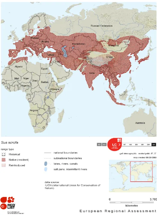
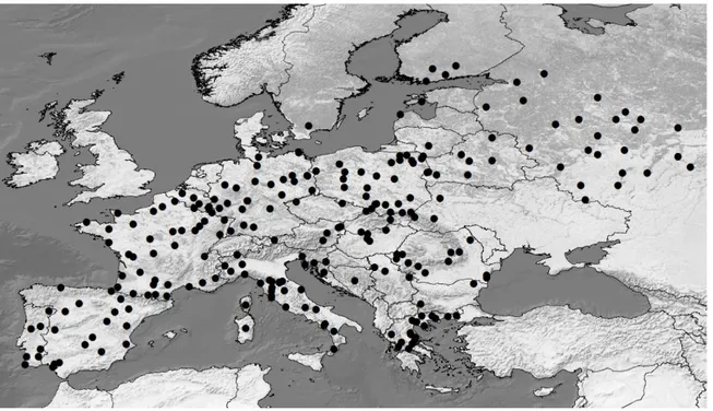
The wild boar, Sus scrofa (Linnaeus, 1758), has one of the most widespread terrestrial distributions of all mammals, occurring in all Europe and Asia (Figure 1). In some areas, boars can cause damages to agricultural cultivations and natural ecosystems; over-hunting and changes in land use have resulted in the range fragmentation and its extermination though the British Isles, Scandinavia, parts of North Africa, Russia, and northern Japan (Groves & Grubb 1993). In recent years, its range has been greatly expanded by humans especially after the Second World War, when the occurrence of the wild boar increased almost everywhere in Europe. Factors like global warming, changes in agricultural practices, restocking and reduced number of predators, directly influenced the recent population growth of the wild boar (Scandura et al. 2008).
The wild boar has by far the largest range of all pigs. It occurs throughout the steppe and broadleaved forest regions of the Palearctic, from western Europe to the Far East, extending southward as far as North Africa, the Mediterranean Basin and the Middle East, through India, Indo-china, Japan (including the Ryukyu Chain), Taiwan and the Greater Sunda Islands of southeast Asia (Groves & Grubb 1993). Besides the great geographical distribution, the Eurasian wild boar also occurs in a variety of temperate and tropical habitats, from semi-desert to tropical rain forests, temperate woodlands, grasslands and reed jungles, and often ventures onto agricultural land to forage. It has been extinct in the British Isles since sometime in the 17th century, despite attempted introductions of new stock from Europe, although recently animals have escaped from captivity and have established in the wild (there are at least three small wild populations in England, on the Kent/East Sussex border, in Dorset, and in Hereford (Oliver & Leus 2008)). It is also extinct in southern Scandinavia, over extensive portions of its recent range in west-central and eastern parts of the former Soviet Union, and in northern Japan (Groves & Grubb 1993). The species was last reported in Libya in the 1880s, and it became extinct in Egypt in 1902 (Oliver & Leus 2008).
Depending on the author classification, at least 16 subspecies of wild boar can be identified, reaching up to 26 (Genov 1999; Mayer & Brisbin Jr 2008). The most accepted subspecies list (Groves & Grubb 1993) distinguishes four “subspecies groups”, based on both geographic and morphological criteria:
9 1. “Western races” in Europe (scrofa and meridionalis), North Africa (algira) and the Middle East (lybicus), extending at least as far east as Central Russia (attila and nigripes);
2. “Indian races” of the sub-Himalayan region from Iran in the west (davidi) to north India and adjacent countries as far east as Myanmar and west Thailand (cristatus), and south India and Sri Lanka (affinis and subsp. nov.);
Figure 1 – Distribution of the wild boar in Europe and Asia, with indication of the range type. From Oliver & Leus (2008)
10 3. “Eastern races” of Mongolia and the Russian Far East (sibiricus and ussuricus), Japan (leucomystax and riukiuanus), Taiwan (taivanus), to south-east China and Viet Nam (moupinensis);
4. “Indonesian race” (or banded pig) from the Malay Peninsular, Sumatra, Java, Bali and certain offshore islands (vittatus).
The wild boar is omnivorous, though stomach and fecal contents analyses indicate that vegetable matter, principally fruits, seeds, roots and tubers, constitutes about 90% of the diet (Groves & Grubb 1993). It is believed that the food availability (including the presence of acorns, Quercus sp.) is one of the essential factors responsible for shaping year-to-year variation in wild boar population density (Melis et al. 2006). Analysis of long-term records of wild boar densities in the Bialowieza forest in Poland and of hunting bags in Germany showed that the presence or absence of the mast of deciduous trees, such as beech Fagus sylvatica L. and oak species Quercus L. were the dominating factor determining yearly population growth rates (Bieber & Ruf 2005).
The litter size is usually between 4 and 7 piglets in western Europe, and reports from Iraq and Armenia cite 5 to 7-10 piglets as being usual (Sommer et al. 2009). Litter sizes of wild boar in Mediterranean countries such as Spain or Italy are generally smaller than those observed in more eastern countries of Europe, probably due to a drier climate and lower resource availability (Servanty et al. 2007).
According to Groves & Grubb (1993), boars are normally most active in the early morning and late afternoon, though they become nocturnal in disturbed areas, where activity usually begins shortly before sunset and continues throughout the night. A total of 4 to 8 hours are spent foraging or traveling to feeding areas. Radio telemetry studies indicate that boars generally travel up to 10 km per night. Social groups tend to be faithful to a resting place (Goulding 1998).
In most of its range, the wild boar is considered as an environmental pest, since local populations are reported to be increasing in number, especially in countries where the Islamism is the predominant religion (Oliver & Leus 2008). Wild boars are known to cause damages to agriculture, and in some areas (e.g., in Japan) farmers are paid to hunt them (Oliver & Leus 2008). On the other hand, in some countries it is considered as a valuable game resource and populations are sustained by artificial restocking. Nevertheless, some populations of wild boar are under serious extinction risk. The Japanese Ryukyu pig (S. s. riukiuanus) is included in the IUCN Red List of Threatened Animals, where it has been granted the status of “vulnerable” since 1982 (Oliver & Leus 2008).
11 In Italy, before the 1500’s, the wild boar was present throughout the country, but during the end to the 16th century due to hunting pressure it has been progressive declining. Local extinctions were reported in Trentino (17th century), Friuli and Romagna (18th century) and Liguria (1814), with the lowest densities been reported before the Second World War (Vatore et al. 2007). After the 1950’s a general increasing of the population was observed, in part due to the recovery of forests used before for agriculture, placement of artificial feeding sites, decrease in predator numbers, global warming, reintroductions, and decreased hunting pressure (Vernesi et al. 2003). Currently in Italy the wild boar is present in 90 provinces out of 103, with a population estimated in 300,000 to 500,000 individuals (Vatore et al. 2007). The few areas that the boar is currently absent are in the Adriatic coast and in the Alpine arc in altitudes beyond the limit of vegetation trees.
Genetic studies
Cytogenetics
European and Asian boars differ in their chromosome number. Asian wild boars have 2n = 38, while Europeans have 2n = 36. The difference between the two karyotypes is a single centric fusion between chromosomes 15 and 17, resulting in the 2n = 36 karyotype. European populations exhibit numerical polymorphism with 36, 37 and 38 chromosomes. Karyotypes 2n = 37 arise from crossings between individuals with karyotype 2n = 36 and 2n = 38. The probable ancestral condition was 2n = 38, which is the most common karyotype in Asia wild (and domestic) pigs. Thus, the chromosomal number 2n = 36 is a derived state that is now very common in Europe (Scandura et al. 2011a).
Although no detailed study was done in a continental scale, a recent review on wild boar genetic diversity (Scandura et al. 2011a) showed that the distribution of the chromosomal number in Europe does not show a clear geographical border, with the Netherlands, Spain, Italy, Poland, Russia, Lithuania, Byelorussia being polymorphic for chromosome number (2n = 36, 37, 38); while Austria, Germany and France exhibited only 2n = 36; and Corsica and Yugoslavia only 2n = 38.
Genetic structure and variability in molecular markers
Phylogeographic studies have been made in populations worldwide, although only one study (Larson et
12 one marker of the mitochondrial DNA (mtDNA), the control region (CR), with only a few using the mitochondrial gene Cytochrome B, nuclear microsatellites (Scandura et al. 2008; Vernesi et al. 2003) or the Y chromosome (Ramirez et al. 2009). Recently, also the complete genome of ten wild boars (six Europeans and four Asian) and several domestic pigs were published (Groenen et al. 2012). Totaling 60,000 single nucleotide polymorphisms (SNPs), a SNP chip was also developed by Amaral et al. (2011) from genome sequences of European pigs and wild boars.
The most used marker for phylogeographic studies in wild boars is the control region of the mtDNA. Studies that used this this DNA fragment were able to identify numerous geographic groups, several in Asia, one in the Middle East, and two in Europe (Figure 2). Within the Asian group at least eight different subgroups can be observed, while within the European group one large subgroup is widespread in the entire continent (E1), and another subgroup is restricted to Italy (E2) (Larson et al. 2005). Besides the European continent, the E1 lineage is present in the Near East (although this region has its specific clade) and North Africa, but was not observed in Asia (Hajji & Zachos 2011; Ramirez
et al. 2009). Based on molecular clock, the time most recent common ancestor (TMRCA) between the
Asian clade and E1 was dated back to 900,000 years before present (BP), while the clades E1 and E2 separated at least 50,000 years BP (Scandura et al. 2008).
The strikingly difference between Asian and European wild boars is also observed in the Y-chromosome (Ramirez et al. 2009) and nuclear microsatellites. As a general pattern, Asian boars have more diversity than their European con-specifics. According to Scandura et al. (2011a) this pattern of genetic variation may reflect past expansion dynamics from the origin area, the south-eastern Asia. Within Europe, two main studies were done involving samples of the entire continent (Larson et al. 2005; Scandura et al. 2008). Both studies, using a small portion of the CR (663 bp and 411 bp, respectively), found one clade distributed from Portugal to Poland and one clade exclusively found in continental Italy and Sardinia (Figure 2). The European clade shows two core lineages, denominated A and C (Larson et al. 2005, Figure 3). The haplotypes A and C are found in high frequency in the continent and are separated by one transversion (Figure 3). In a network analysis, Larson et al. (2005, Figure 3) found that all the other E1 haplotypes are distributed in a star-like pattern around these two core haplotypes, which is consistent with a population expansion analogous to the one seen in cattle (Troy et al. 2001). In a meta-analysis involving recent published sequences, Scandura et al. (2011a) found that C-side haplotypes (sequences directly derived from the C haplotype)
13 Figure 2 – Worldwide distribution of mitochondrial clades of wild boars. From Larson et al. (2005). are more commonly found in Iberia and eastern Europe, while A-side haplotypes are found in Central Europe and Italy.
Two studies genotyped diverse microsatellite loci in continental populations. Vernesi et al. (2003) showed that Hungarian and Italian samples from natural parks (Maremma and Castelporziano) were composed by homogenous clusters, while boar from Florence, which was greatly affected by reintroductions, were genetically intermediate with several hybrids. Ramirez et al. (2009) investigated boar populations from Europe, Near East and North Africa and could not find any strong differentiation between these three regions, with several shared alleles.
14 Figure 3 – Network depicting the relationship between the haplotypes found in Europe. Colors within the nodes: yellow, domestic; green, wild; orange, feral; blue, unknown status; and red, inferred intermediate haplotypes not represented by any sampled pigs. From Larson et al. (2005).
In more geographical restricted studies, Alexandri et al. (2012), Ferreira et al. (2009), Velickovic et al. (2012), Nikolov et al. (2009), Scandura et al. (2011b) and Alves et al. (2010) studied diverse European populations. All studies found local geographic groups: Ferreira et al. (2009) using six microsatellite loci found that Portuguese populations could be subdivided in North, Centre and South (result also supported by van Asch et al. (2012) using mtDNA). Alves et al. (2010) using 660 bp of the mitochondrial CR showed that the Iberian population constitute a different gene pool compared to other European populations. Alexandri et al. (2012) using a CR fragment of 637 bp identified a total of 62 unique haplotypes in Balkan wild boars that formed two structured groups: one in central Greece and one in north Greece/Bulgary. Interestingly the Greek island of Samos was composed by only Near Eastern haplotypes, probably due to its geographical proximity to the Anatolian Peninsula. In the three studies, only E1 sequences were found in continental Europe (with an exception of one sample from northern Greece which possessed an Asian haplotype). Within Bulgaria, Nikolov et al. (2009) found two distinct clades typing 10 microsatellites, one north and one south-west of the Thracian Valley. Using only four microsatellite loci, Velickovic et al. (2012) reported that Croatian/Serbian populations
15 were differentiated from Bosnian wild boars. Scandura et al. (2011b) typed more than two hundred wild boars across Sardinia for 10 microsatellites and found three regionally structured groups inside the island.
The Italian clade, E2, have at least five single nucleotide changes in comparison to the rest of the European haplotypes (Scandura et al. 2008). Taking into consideration only modern sequences, the E2 clade is only found in the peninsular Italy and Sardinia, with an especially high frequency in two areas: Castelporziano Reserve and Maremma Regional Park. The main reason for this strong genetic discontinuity in Italy is probably the presence of the Alps, which is a physical barrier to the dispersal of individuals (Scandura et al. 2011a; Scandura et al. 2008). In contrast, Sardinian wild boars are strongly differentiated from any other continental population, including the Italian populations (Scandura et al. 2011b; Scandura et al. 2008). Using microsatellites markers (Scandura et al. 2011b) showed that this island population have almost “private” genetic components, constituting a different group, even if part of this strong differentiation may have arisen due to introgression with exotic wild populations or local domestic stocks. Regarding the mtDNA, Sardinian wild boars have a high frequency of private alleles (Scandura et al. 2008).
Several studies at different geographical scales and using different markers tried to estimate the demographic dynamics of the European populations using genetic data. For example, Ferreira et al. (2009) concluded that all three Portuguese populations distinguished by microsatellite markers showed a size decrease, and Alves et al. (2010) analyzing both Portuguese and Spanish populations with mtDNA failed to find any demographic expansion. In eastern European wild boars, Alexandri et al. (2012) failed to find any demographic expansion in Central Greece, although an excess of low-frequency polymorphisms was detected, but for the Greece/Bulgarian population it was possible to see a sign of growth/expansion. In studies using more wide range samples, Larson et al. (2005) when analyzing only E1 haplotypes found a star-like network compatible with a recent population expansion, and neutrality tests using both wild boar and domestic pigs mtDNA sequences were consistent with a population expansion. Scandura et al. (2008) found a sign of expansion when analyzing European sequences (excluding Italy), while the Italian population did not show any past demographic expansion for both E1 and E2 clades. The different results obtained by these studies in different geographical areas exemplify the complexity of the European demographic history and the need of a global analysis.
16 The publication of the genome of several European wild boars also shed some light into the demography of the wild boar (Groenen et al. 2012). Asian wild boars showed much more segregating SNPs in the genome, when compared to European. The differentiation between these two lineages is also clear at the genomic level, with 1,272,737 fixed differences between them. Phylogenomic analysis of complete genome sequences from wild boars and six domestic pigs revealed distinct Asian and European lineages, with an estimated split date during the mid-Pleistocene 1.6 – 0.8 million years ago, an estimation in accordance with previous mtDNA studies.
The contribution of ancient DNA
Only two studies involving museum/ancient samples in European wild boar were published so far (Larson et al. 2007a; Larson et al. 2005), although other studies that involves the Asian continent (Larson et al. 2007b; Larson et al. 2010) and the Middle East (Ottoni et al. 2012) have been published. In a worldwide phylogeographic study, (Larson et al. 2005) included sequences from museum samples, although most of them were from Anatolian or Asian origin. Among the European ones, 21 sequences were included, and only eight were not from Italy, Sardinia or Corsica. Within these three sites, they all showed typical European alleles (A-sided haplotypes). Within continental Italy, six sequences from the Maremma Regional Park were included: they were typical Italian although the haplotypes are not currently found in wild boars from this region. In Corsica and Sardinia, three typical A-sided European haplotypes were found.
Using ancient DNA, Larson et al. (Larson et al. 2007a) investigated the Neolithic transition in Europe. Diverse sites throughout Europe from 11,000 BC to 1,500 AD (spanning a total of 13,000 years) were included in this study. Differently from the modern pattern, Italian E2 haplotypes were found in Croatia 9,000 years ago; Near Eastern haplotypes were found in wild boars from 5,900 BC – 3,900 BC in Germany, France and Romania. This means that Near Eastern pigs arrived in Europe during the Neolithic, but no genetic signature is detected in either modern European domestic breeds or wild boar populations. The same is valid for the Italian haplotypes, around 9,000 years ago they could be found outside the Italian peninsula, but no genetic signature is currently detected north of the Alps. Besides these two exceptions, all other haplotypes in Europe during this time span were typical E1.
In a more detailed study, (Ottoni et al. 2012) investigated the history of wild boar in Near East and Anatolia. In a previous study, (Larson et al. 2007a) showed that by 3,900 BC, all domestic pigs in
17 Europe possessed haplotypes only found in European wild boar. This pattern was probably due to introgression with local female wild boar into imported domestic stocks. After the genetic turnover in Europe, ancient samples from Armenia indicated that European pigs were present in the Near East by 700 BC until the end of the Iron Age, where they replaced indigenous Near Eastern domestic pigs. Ottoni et al. (Ottoni et al. 2012) showed that European wild boars arrived in Near East almost 1,000 years before the estimated data from Larson et al. (Larson et al. 2007a). Already at the early Middle Bronze Age European haplotypes were present in Armenia, introduced by humans. They also demonstrated how the frequency of pigs with European ancestry increased rapidly from the 12th century BC, and by the 5th century AD domestic pigs exhibiting a Near Eastern genetic signature had disappeared across Anatolia and southern Caucasus.
Translocations, restocking and hybridization with domestic pigs
In the last few centuries, habitat loss and hunting pressure have led to the decline of several European populations, with extinctions in a few regions such as the British isles, Scandinavia, and several Italian and western Russian areas. In order to restock areas where the population declined, events of translocation and/or release of wild boars from other areas were done. After two centuries of demographic decline, reintroductions of the wild boar in central Italy began in the 1950’s (Apollonio et
al. 1988). Even though registers indicated that individuals from central Europe were used to restock
local populations (from Hungary, Czech Republic and Poland), which almost led to the extinction of subspecies S. s. majori (Vatore et al. 2007), their effective contribution to the Italian genetic pool is not seem when analyzing mitochondrial fragments and microsatellites (Scandura et al. 2008; Vernesi et al. 2003). In the UK, the wild boar became extinct in 1705, and since then, escapes and deliberate release of captive animals (farmed in the UK since the 1980’s) has led to the re-establishment of four known populations totaling 750 – 1000 animals (Hartley 2010). In Spain, the wild boar is still an important game species, with 5,000 boars being shot annually during the hunting season. Due to hunting demand, an unknown number of wild-caught or captive-bred wild boars are imported yearly for restocking, mainly from France (Fernandez-de-Mera et al. 2003).
The hybridization with domestic pigs are also a factor to be considered, wild boars and domestic pigs being fully capable of interbreeding. In central Italy, pigs were occasionally crossbred with wild boar in captivity and hybrids were released for hunting purposes (Randi et al. 1989). Genov et al. (1991)
18 reported that the traditional practice of rearing “domestic” pigs in semi-wild conditions in Bulgaria has resulted in their hybridizing with the wild boar populations in the eastern and north-eastern parts of that country, and that genetically pure wild boars now occur only in the south of the country, where domestic pigs are not reared in the wild.
Translocations and restocking are expected to affect the genetic variation in local populations, especially when distinct genetic groups are being admixed. For the wild boar, the effects of translocation and hybridization with domestic pigs seem to have affected the local populations in different degrees. Vernesi et al. (2003) analyzing Italian and Hungarian wild boar populations with microsatellite markers, suggested a limited impact of reintroductions, with patterns of genetic variation at a macro-geographic scale appear to have been only slightly affected by recent human manipulation, since the effects of ancient demographic events are still detectable. In Sardinia, the wild boar population is supposed to have originated when Neolithic pigs escaped from man’s control and became feral (Scandura et al. 2011b). In their study, Scandura et al. (2011b) found that 11% of the sampled Sardinian wild boars were immigrants or hybrids with continental ancestors.
Besides the influence on the wild boar genetic diversity, translocations and restocking might also have an implication in disease control and parasites distribution. The translocation of French wild boars into Spain for hunting purposes was associated with the transmission of diverse helminth species, once only found in translocated animals and now also found in wild ones (Fernandez-de-Mera et al. 2003). One of the main causes on diseases outbreaks, including swine fever, is associated with the import or translocation of boars and subsequent release into wild for sports hunting (Hartley 2010).
Climate and LGM: the impact on species distribution and genetic variation
Climatic changes in Europe during glaciations
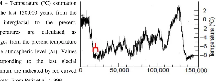
Global climate has fluctuated greatly during the past three million years, leading to recent major ice ages. The Earth’s climate became cooler through the Tertiary (64 million years (Myr)) with frequent oscillations that increased in amplitude and lead to a series of major ice ages during the Quaternary (2.4 Myr to the present). Along with other measures, the extraction of ice cores of 2 km in length are particularly important in the study of the temperature changes. The analysis of annually layered snow for entrapped gases, isotopes, acidity, dust and pollen can cover over 400 kyr (thousands of years ago)
19 (Petit et al. 1999), but most go back 125 kyr from the present to the previous (Eemian) interglacial. The Greenland (Artic) and Vostok (Antartic) ice cores are particularly informative, offering fine temporal resolution and continuity (Figure 4).
While the Antarctic ice cap grew from the Oligocene (35 Myr ago), the Arctic ice cap became established about 2.4 Myr ago. From then until 0.9 Myr ago, the ice sheets advanced and receded with a roughly 41,000 year cycle; thereafter they have followed a 100,000 year cycle and became increasingly dramatic. Such periodicity suggests a controlling mechanism, and the Milankovitch theory proposes that the regular variation in the Earth’s orbit around the sun are the pacemakers of the ice-age cycles, with the 41,000 year cycle being caused by a oscillation of earth’s axial tilt, and the 100,000 year cycle happening due to a eccentricity of Earth’s orbit (Bennett 1990). The Milankovitch cycles control the pace of Quaternary ice ages, with the 100,000 year cycle eccentricity cycle dominate in the Late Quaternary and the 41,000 year cycle dominant in the early Quaternary.
These several climatic oscillations produced great changes in species distributions, with species going to extinction over large part of their range, or dispersing into new locations, or surviving in refugia and then expanding again. The effects of the glaciations varied according to latitude and topography (higher latitudes and altitudes suffered more from the glaciations effects), and temperate regions suffered more than tropical regions (Hewitt 2011). Regarding the European continent, the last full glacial period (from the Eemian interglacial around 135 kyr to present) is the best understood, and in particular the last warming from full glacial conditions around 18,000 years ago (18 kyr) through the current warm interglacial climate (Hewitt 1999).
Fig 4 – Temperature (°C) estimation for the last 150,000 years, from the last interglacial to the present. Temperatures are calculated as changes from the present temperature at the atmospheric level (ΔT). Values corresponding to the last glacial maximum are indicated by red curved brackets. From Petit et al. (1999).
20 During the Last Glacial Maxima (LGM), which occurred between 23 kyr to 18 kyr, a great part of Europe was covered by an ice sheet that extended to 52°N, and permafrost south to 47°N. All the major mountains chains had extensive ice caps. Between the main ice sheet and the southern mountain blocks (Alps, Pyrenees, Cantabrians, Transylvanians and Caucasus) was a plain of permafrost, tundra and cold steppe, which extended eastwards across Russia and the Urals (Hewitt 1999). From about 16 kyr, the climate warmed and the ice retreated, until 11 kyr when the Younger Dryas period shifted the temperatures and ice readvanced in some areas. Around 13 kyr, there is some evidence of spread of pine, oak and elm in the western Atlantic fringe to Britain, Ireland and Scotland due to water currents or animals (Hewitt 1999). Once this period came to an end around 10 kyr, the climate warmed again and around 6 kyr the vegetation pattern broadly resembled what is seen today. In the far north the Scandinavian ice sheet remained only on the highlands by 8 kyr; similarly, the glacial blocks on southern mountains like the Pyrenees and Alps had shrunk and represented less extreme barriers to cross.
The impact of climate change in species distributions
Recent analysis of deep ice cores in Greenland revealed a dramatic switch in the temperature through the ice age and the Eemian interglacial. Average temperatures would seem to have changed 10-12% over 5-10 years and lasted for periods of 70-5000 years (Hewitt 1999). Such massive temperature change combined with geography greatly influenced the species movements and distributions in Europe during the LGM. Species went extinct over large parts of their ranges, some dispersed to new locations, some survived in refugia areas and then expanded again (Hewitt 2000).
Species are expected to respond to climate variation, reducing or increasing their ranges/abundances accordingly to the temperature variation and tolerance to warm/cold weather. During the LGM, species all over the world responded to the climate change, with less or more intensity depending on the latitude and altitude (Hewitt 2000) and on their cold tolerance. In Europe, the study of the Quaternary phylogeography is based on fossil data, relying on pollen cores and beetle fossil records, to describe the changes in species distributions through the last Ice Ages (Hewitt 1999; Hewitt 2004). This is most detailed for the last glacial cycle (120,000 years ago), which is complemented by recent ice-core data on paleoclimates.
21 Currently, the reconstruction of past climate data in Europe is heavily based in pollen data, which directly reflects the distribution of trees during the glacial period. One of the methods of reconstruction involves the quantitative reconstruction of climatic parameters from fossil pollen data based on a modern data set (based on plants functional type and biome concepts) for calibration or on reference to modern analogs (Peyron et al. 1998).
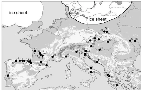
Fossils from animals can also help to reconstruct how the glacial period influenced species distributions (Figure 5). Fossils are a direct evidence of a glacial refuge: only fossil remains of temperate species1 dated to the LGM can indicate glacial refuge; the closer the fossils are dated to the culmination point of the LGM, the more significant is the evidence of a refuge (Sommer & Nadachowski 2006).
Combining pollen data, fossil distribution and DNA evidences from ancient sequences, several studies tried to recover possible refuge areas throughout Europe. Three areas are always recovered as glacial refuge for Mediterranean1 species: Iberia, Italy and the Balkans (Hewitt 2000; Hewitt 1999; Schmitt 2007).
1 Mediterranean species refers to the biogeographic group of last dispersal center, not the recent distribution pattern of a
species - the distribution can reach Scandinavia but it is considered Mediterranean if the last refuge was in the Mediterranean basin expanding northwards in the postglacial. Schmitt T (2007) Molecular biogeography of Europe: Pleistocene cycles and postglacial trends. Front Zool, 4: 11..
Fig 5 – Forty seven archeological sites around Europe with mammal sites associated with the LGM period (radiocarbon dating). Numbers are associated with locations defined in Sommer & Nadachowski 2006.
22 In the case of some cold-tolerant species, northern refuges can also be found, as in the case of several tree and mammal species that were found during the LGM like Slovakia, Hungary, and UK (Stewart & Lister 2001). These cryptic refugia were characterized by small tree patches in buffered local microclimates.
The population shrinking into more southern areas during the LGM is also reflected in the species genetic diversity and the current patterns of diversity distribution across the Europe. Using mainly mitochondrial DNA, several studies tried to investigate the consequences of the temperature decrease during the LGM in European species. These include invertebrates (Habel et al. 2010; Weigand et al. 2012), mammals (Rebelo et al. 2012; Vega et al. 2010) and trees (Svenning et al. 2011).
Migration patterns post-LGM
When the temperature started to increase again, around 16 kyrago, the ice retreated and species started to expand their ranges northwards, out of the refugia (Hewitt 1999). During this period, the temperature warmed rapidly, and populations at northern limits of the refuge range expanded into more relatively large areas of suitable territory. Each species reacted differently to this warming, according to its own responsiveness to environmental conditions such as barriers, habitat conditions and prior colonizers. The differential response was determinant on how the species expanded, which route they took based on the presence of barriers, suitable habitat, and on how long they took to expand northwards of the refugia.
Four general postglacial patterns from southern refugia are usually defined for the European populations: the grasshopper, hedgehog, bear and the butterfly (Schmitt 2007) (Figure 6). These four paradigms reflect the main expansion routes used by European species to expand to northern areas from the three refugia areas after the LGM, with direct consequences on the distribution of the genetic diversity. The hedgehog paradigm shows a postglacial expansion from all three southern European refugia, the bear paradigm reflects an expansion of the western (Iberia) and eastern (Balkans) lineages but trapping of the Italian lineage; the butterfly exemplifies an expansion of the Italian and eastern lineages but trapping of the western lineages; and the grasshopper dispersion example has one major expansion from the Balkans and trapping of Italian and Iberian lineages.
23 The four paradigms are frequently repeated in many animal and plant species, with various examples in the literature. One interesting pattern that arises when comparing the fours paradigms is the differential influence of barriers in the species dispersion, especially the presence of mountains and how they limited the migration from refuge areas. Carpathians, Alps and Pyrenees are the three greatest mountain chains in Europe, and directly influenced the post-colonization routes from the Balkans, Italy, and Iberia, respectively. In a review of post-migration routes, Hewitt (1999) estimated that the Alps were a greater barrier when compared to the other two mountain chains, since it blocked the expansion of 8 out of 11 species. The Pyrenees seem to be less of an impediment, blocking 4/11 species, while only two species did not expand from the Balkans but probably due to earlier colonizations from the East (Hewitt 1999).
The fact that the Alps are a greater barrier to post-glacial colonization affected current genetic distribution throughout Europe. For the majority of species studied, Italy is the refuge area with more unique haplotypes, because once the individuals were isolated in the refuge areas and started to differentiate (accumulate unique haplotypes), they remained isolated by the presence of the Alps, while individuals from the Iberian and Balkans refugia expanded north.
24 Figure 6 – Patterns of postglacial expansion from southern refugia. Red arrows represent the expansion from each of the refugia, while white forms depict putative barriers. A) Hedgehog, B) Grasshopper, C) Bear, D) Butterfly.
The rapid northward expansion across the European plains occurred when the climatic conditions became more suitable, and different genetic consequences are expected due to the presence of mountains in southern parts. The dispersal at the leading edge of a refuge would likely be by long distance dispersants that set up colonies far ahead from the main population. These pioneers could expand rapidly to fill the area before significant numbers of dispersants arrived, and so their genes would dominate the new population genetic diversity. A series of founder effects would be repeated many times during an expansion distance, leading to a loss of alleles and to higher homozygosity in the new populations. This predicts that a rapid continued expansion would produce large areas of reduced genetic diversity in northern Europe. A rapid expansion from one refugia would also hamper the expansion from other refugia, since the pioneer area would already be colonized and a migrant from the
A
B
25 behind the front of expansion would not contribute to the new population nor influence its genetic diversity.
Species Distribution Models (SDMs)
Species distribution models estimate the relationship between species records at sites and the environmental and/or spatial characteristics of those sites (Franklin 2009). They are widely used for many purposes in biogeography, conservation biology and ecology, including species extinctions, speciation mechanisms, plant diversification, ecological niche conservatism, past distribution of different taxa (including extinct ones), location of Pleistocene refugia, biodiversity hotspots and historical migration pathways (Nogués-Bravo 2009).
SDMs are also referred to as habitat suitability models, describing the suitability of habitat to support a species. The concept of habitat suitability is closely related to the idea of a resource selection function from wildlife biology. A resource selection function (RSF) is any function (for example, from a statistical model) that is proportional to the probability of habitat use by an organism. If a RSF is proportional to the probability of use, then a SDM could be said to predict the likelihood of an event (species) occurs at a location, that is, the probability of species presence (Franklin 2009).
SDMs describe empirical correlations between species distributions and environmental variables. In order to successfully model a species distributions the following elements need to be followed:
A theoretical model controls the species distribution over time and space, and at different scales, and the expected form of the response functions;
data on species occurrence (location) in geographical space; digital maps of environmental variables representing those factor determining habitat quality (generally derived from remote sensing and stored in GIS);
a model linking habitat requirements to the environmental variables; tools for applying the model (rules, thresholds, etc);
data and criteria to validate the predictions and a way to interpret error or uncertainty in the analysis (see diagram below).
26 But after a map of predicted occurrence is drawn from the data, the modeled distribution reflects which kind of niche concept? In other words, what exactly is being modeled? This topic has been approached in various studies (Franklin 2009; Phillips et al. 2006; Symonds & Moussalli 2011), if the fundamental species niche (response of species to environment in absence of biotic interactions such as competition or predation), the realized niche (the environmental dimensions in which species can survive and reproduce, including the effects of biotic interactions) or the probability of habitat use (potential distribution) are the results of the SDMs. Most studies identify a description of the realized niche as the outcome of SDM (Austin 2002; Guisan & Thuiller 2005), because data on actual species occurrence are usually used in modeling, and so the model extrapolates in geographical space those conditions associated with species abundance or occurrence in the environmental “hypervolume” (Figure 7). When this realized niche described by the statistical model is mapped in geographical space it represents the potential distribution or habitat suitability (Araujo & Guisan 2006). But depending on the method of SDM, different outcomes can be proposed in relation to which kind of niche is being modeled. It has been suggested that environmental envelope-type models using presence-only data tend to depict potential distribution (suitable habitat) and are more suitable for extrapolation while more complex models that discriminate presence from absence (logistic regression, GAM, decision trees – such as random forests) tend to predict realized distributions (occupied habitats), and are more suitable for interpolation (Franklin 2009). A different view, discussed in (Phillips et al. 2006) suggests that
27 models based on occurrence localities, called niche-based models, represents the realized niche since it is an approximation of the species’ realized niche. Niche-based models are drawn for a source habitat, rather than a sink habitat, which may contain a given species without having the conditions necessary to maintain the population without immigration. Then, by definition, environmental conditions at the occurrence localities constitute samples from the realized niche.
The climatic niches of species are potentially the result of inheriting the climatic niches of their ancestors, and the result of adaptation of species to past and current climatic conditions that allows them to persist. One of the main theoretical assumptions for transferring the projections of SDMs through time (or extrapolation) is the temporal stability of climatic niches (Nogués-Bravo 2009). These models assume a non-significant evolutionary and/or ecological change in a species niche as a response to changing environmental conditions through time. Nevertheless, recent studies suggests that niche shifts have occurred for some species (Pearman et al. 2008a), due to changes in the fundamental niche or because of competition with different species over different periods of time; questioning the premise of niche stability. Whether the niche shifts are a general pattern may depend on the scale: in a geographical scale (regional vs. continental) or temporal (100 years; 10,000 years or 1,000,000 years). Although the influence of the temporal scale remains an unanswered question (Nogués-Bravo 2009), several studies that modeled the potential distribution over different time scales proposed different ways to test the niche stability over time, including the presence of fossils (Nogués-Bravo et al. 2008), lineage membership (Peterson & Nyari 2008), multivariate techniques (Pearman et al. 2008b) and climatic response curves for past and present conditions (Rodriguez-Sanchez & Arroyo 2008).
Figure 7 – Example of an environmental “hypervolume”. The environmental space (right) is a consequence of mapped species (letters) in environmental data (left). Note that inter-site distance in geographic space might be quite different from those in environmental space – a and c are geographically close, but not environmentally.
28
Presence-only methods
In the last two decades, there have been many developments in the field of species distribution modeling, and multiple methods are now available. A major distinction among methods is the kind of species data they use. Where species data have been collected systematically – for example in formal biological surveys in which a set of sites are surveyed and the presence/absence or abundance of species at each site are recorded – regression methods can be used. However, in most cases where only presence-data is available (no absence records), specific approaches are required (Franklin 2009). Models that fit presence-only data predict the relative likelihood of a species presence in a given site, or the relative habitat suitability (Franklin 2009). One of the first systems used for species presence modeling, BIOCLIM (Adamic et al. 2010; Eckert et al. 2008) used a simple “hyper-box” classifier to define species potential range as the multi-dimensional environmental space bounded by the minimum and maximum values for all presences (Figure 8). In other words, the presence of a species is closed inside a box, and its limits are given by the data observed, and the results are a binary classification in suitable or unsuitable habitat. This method is current implemented in the DIVA-GIS software and is still widely used for presence estimation (Bartos et al. 2010; Carranza 2010; Maillard et al. 2010; Wotschikowsky 2010), although with some recent improvements (Franklin 2009). One refinement of this method is the HABITAT (Kusak & Krapinec 2010), which encloses the presence points in a convex hull (Figure 8).
Genetic algorithms are also used for the estimation of a species presence. It is named because a population of classification rules is generated and then the rules “evolve” by a process analogous to natural selection until an optimal solution is reached (Franklin 2009). This approach is useful when there is a large search space for a solution and where there are complex relationships between
Figure 8 - Graphical representation of environmental envelopes shown for two environmental variables (X1 and X2). The
b’s represent the model used by BIOCLIM,
while the a’s represent the model used by HABITAT.
29 variables. This genetic algorithm framework is implemented in the stand-alone software Desktop GARP (Genetic-Algorithm for Rule-set Production, Stockwell & Peters 1999). The classification is based in a series of population of rules generated for determining the species presence/absence. Rules are developed by searching for appropriate conditional probabilities and the resulting model is expressed in terms of conditional decision (Franklin 2009). For example, a species X is present if annual rainfall is >20 cm and average July temperature <14° C. The GARP classification that first generates a set of rules is based in four different methods, including a “BIOCLIM-type” rule. Because the output of GARP is stochastic, it is typical to run the model multiple times, and then average a subset of the best models. The proportion of models predicting presence for an observation (a single pixel) can be interpreted as the probability of occurrence.
General purpose statistical methods such as generalized linear models (GLM) and generalize additive models (GAM) are commonly used for modeling with presence-absence datasets (Franklin 2009). Recently, they have been applied to presence-only situations by taking a random sample of pixels from a study area, known as “background pixels” or “pseudo-absences”, and using them in place of absences during modeling (REF).
Maxent
One other approach to the presence-only data is the Maximum Entropy modeling (MaxEnt, Phillips et
al. 2006). As a general purpose, it is a method for making predictions from incomplete information
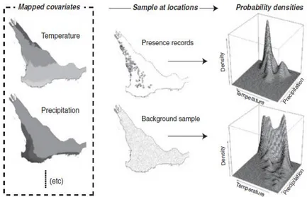
(Baldwin 2009; Phillips et al. 2006). The idea of Maxent is to estimate a target probability distribution by finding the probability distribution of maximum entropy (i.e., that is most spread out, or close to uniform), subject to a set of constraints that represent the incomplete information about the target distribution, which is estimated from a set of species presence observations (Phillips et al. 2006). Maxent has been described as a generative modeling approach that models the species distribution directly by estimating the density of environmental covariates conditional on species presence (Elith et
al. 2011). Environmental factors relevant to habitat suitability (climate, topography, prey presence, etc)
can be considered as independent variables, and in a model for estimating a given species potential distribution they can be called covariates, predictors or inputs. In the case of Maxent, basis function and other transformation of available data are termed features (the expanded set of transformations of the original covariates) (Elith et al. 2011). The features are formed “behind the scenes”, in a similar way as in regression, where the model matrix is augmented by terms specified in the model. Since the
30 fitted function is usually defined over many features, in most models there will be more features than covariates (Elith et al. 2011).
Previous descriptions of the Maxent model were based in a strict machine-learning terminology (Phillips et al. 2006). However, a recent paper published by (Elith et al. 2011) described the model using a statistical terminology and notation, and this was the terminology chosen to describe the Maxent model.
Maxent uses the conditional density of covariates at the presence sites, f1(z), and the background
sample (a finite sample of points from the map with associate covariates), to estimate the ratio f1(z)/f(z).
It does this by making the estimate of f1(z) that is consistent with the occurrence data; despite many
possible distributions, it only chooses the one that is closest to f(z) (the marginal density of covariates across the study area). Minimizing the distance from f(z) is sensible, because f(z) is a null model for
f1(z): without any occurrence data, there would be no reason to expect that a species prefer any
particular environmental conditions over another, and as a consequence the prediction would be no better than predict that the species occupies an environmental condition proportional to their availability in the landscape. In Maxent, the distance from f(z) is taken to be the relative entropy of f1(z)
in respect to f(z).
The use of background data informs the model about f(z), the density of covariates in the region, and provides the basis for comparison with density of covariates occupied by the species (f1(z)). Constraints
are imposed so that the solution is one that reflect information from the presence records. For example, if one covariate is summer rainfall, then constraints ensure that the mean summer rainfall for the estimate of f1(z) is close to its mean across the locations with observed presences. The species’
distribution is thus estimated by minimizing the distance between f1(z) and f(z) subject to constraining
the mean summer rainfall estimated by f1 (and the mean of other covariates) to be close to the mean
31 Phillips et al. (2006) outlined some advantages and disadvantages of Maxent for SDM compared to other methods. Maxent only requires presence data plus environmental information for the whole study area. It can use both continuous (e.g. climatic data) and categorical (e. g. predator presence/absence) data. The results are amenable to interpretation on the form of the environmental response functions. Its efficient deterministic algorithms have been developed that are guaranteed to converge to the optimal (maximum entropy) probability distribution, which also makes it very robust to limited amounts of training data (small samples). The output is continuous, allowing fine distinctions to be made between the modeled suitability of different areas. Some drawbacks of the method are: it is not a mature statistical method as GLM or GAM; its probabilistic models can lead to very large predicted values for environmental conditions outside the range present in the study area; and is not available in standard statistical packages (although a stand-alone and user friendly software was developed and recently the R package dismo also incorporated Maxent estimations).
Maxent has increasingly been used in ecological studies, for estimating species richness (Fløjgaard et
al. 2009; Graham & Hijmans 2006), invasive species (Elith et al. 2010), climate change effects on
Figure 9 – Schematic representation of the probability densities relevant for the model estimation in Maxent. The maps on the left are examples of covariates. In the center are the locations of the presence and background samples. The density estimates on the right show the distribution of values in covariate space for the presence (top) and background (bottom). In a simple model that could represent, respectively, the densities f1(z) and f(z). From Elith et al. (2011).
32 species distributions (Symonds & Moussalli 2011), extent of occurrence (Pearson et al. 2007), climate constraints in species distributions (Wollan et al. 2008). One of the increasing uses of Maxent is to estimate past species distributions, and how past climate changes affected the species distributions in confront to their current distribution (Bartos et al. 2010; Nogués-Bravo 2009; Rebelo et al. 2012; Svenning et al. 2011; Vega et al. 2010). Most studies estimate the effect of the Last Glacial Maximum, with only few studies estimating in other time periods, as the late Pliocene (Rodriguez-Sanchez & Arroyo 2008), mid-Miocene (Varela et al. 2010) and other periods between the last Interglacial (around 120 ka) and the present (Nogués-Bravo et al. 2008).
One reason why Maxent is becoming increasingly popular is because it performs extremely well in predicting occurrences in relation to other common approaches (particularly compared to GARP (Ramayo et al. 2011)). In studies comparing the ability of diverse modeling methods to predict potential future/past distributions (i.e. extrapolation) of diverse species, (Fang et al. 2009) found that Maxent performed considerably poorer than GARP (but Phillips (2008) questioned the experimental design). Elith et al. (2010) compared diverse methods with Maxent (GLM, GAM and boosted regression tree), which aim to minimize extrapolation errors and assess predictions against prior biological data. Their results show that controlling the fit of models and integrating information from mechanistic models can enhance the reliability of correlative predictions of species in novel settings.
33
Chapter 2
Objectives
The objectives of this thesis are:
Describe how the mitochondrial DNA diversity if distributed throughout the European continent
Identify structured populations/groups
Characterize how much the European wild population is influenced by translocations and hybridization with pigs
Check if the current subspecies classification is corroborated by mtDNA analysis
Describe how the Last Glacial Maximum affected the wild boar populations, and how it reflects in today’s genetic distribution
Identify the main refuge areas for the wild boar during the LGM
Characterize the populations/groups responsible for the post-LGM colonization of Europe
34
Chapter 3
Methods
Data collection
Several studies involving the European wild boar have been published, although no study approached the genetic diversity in Europe in a wide range. In order to achieve a full description of the genetic diversity throughout the continent, muscle samples provided by local hunters were obtained for 16 countries: Germany, Luxembourg, France, Portugal, Italy, Greece, Croatia, Bosnia, Serbia, Slovakia, Romania, Bulgaria, Poland, Belarus, Ukraine, and Russia. These samples were sequenced and the data were pooled with previous published sequences (description below) to cover the whole European continent.
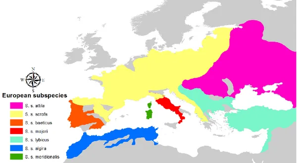
The sampling areas included the range of five subspecies listed in the Mammal Species of the World database (Wilson & Reeder 2005): S. s. scrofa in central-western Europe, S. s. meridionalis in Sardinia and Corsica, S. s. majori in central Italy, S. s. attila in eastern Europe, S. s. lybicus in the Balkans (Figure 10).
Figure 10 – European wild boar subspecies distribution. Each subspecies is shown in a different color. Subspecies ranges were taken from Groves & Grubb (1993).
35 Sequencing
A total of 467 wild boar specimens from 36 locations throughout Europe were sequenced. Total genomic DNA was isolated using a commercial DNA isolation kit (Sigma, Qiagen). Laboratory analyses consisted in amplification of almost the entire control region (CR) using two primers developed by (Alves et al. 2003): Ss.L-Dloop 5’-CGCCATCAGCACCCAAAGCT3’ and Ss.Hext-Dloop 5’-ATTTTGGGAGGTTATTGTGTTGTA3’. Amplifications conditions were set as 35 cycles of 92 °C for 1 min, 62 °C for 1 min, 72 °C for 1 min, followed by a final extension step at 72 °C for 10 min. PCR products were purified by Exo/SAP digestion and a 411-bp fragment was directly sequenced using the forward primer SS.L-Dloop and the BigDye Terminatior kit version 3.1 (Applied Biosystems). Fragments were purified in columns loaded with Sephadex G-50 and run in an ABI Prism 3100 Avant automatic sequencer (Applied Biosystems).
Samples from Tunisia, previously sequenced in a partially overlapping region of the D-loop by Hajji & Zachos (2011), were sequenced for the complementary fragment in order to be fully aligned with European sequences. The sequence protocol was the same as mentioned above.
Electropherograms were visually inspected and base calls edited in FinchTV 1.2. Due to the quality of electropherograms and the shortness of the region, most sequences were obtained with a single (forward) primer. Nonetheless, to assure accuracy of nucleotide identification, a subset of samples was sequenced in the reverse direction and all individuals assigned to singleton haplotypes were sequenced twice, as well as all samples showing doubtful base calls, using the internal reverse primer (Ss.Hint-Dloop 5’-TGGGCGATTTTAGGTGAGATGGT3’).
Data description
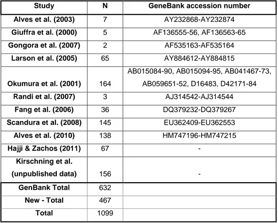
The 467 new sequences were aligned with sequences available in GenBank (Table 1). Sequences from previous studies were added, forming a database with 1099 individuals.
All 1099 sequences were aligned using the ClustalX algorithm implemented in MEGA v. 4.0 (Tamura
et al. 2007). The downloaded sequences represented animals classified as wild Sus scrofa from Europe,
36
Study N GeneBank accession number
Alves et al. (2003) 7 AY232868-AY232874
Giuffra et al. (2000) 5 AF136555-56, AF136563-65
Gongora et al. (2007) 2 AF535163-AF535164
Larson et al. (2005) 65 AY884612-AY884815
Okumura et al. (2001) 164
AB015084-90, AB015094-95, AB041467-73, AB059651-52, D16483, D42171-84
Randi et al. (2007) 3 AJ314542-AJ314544
Fang et al. (2006) 36 DQ379232-DQ379267
Scandura et al. (2008) 145 EU362409-EU362553
Alves et al. (2010) 138 HM747196-HM747215
Hajji & Zachos (2011) 67 -
Kirschning et al. (unpublished data) 156 - GenBank Total 632 New - Total 467 Total 1099 Network
The alignment, corresponding to 1099 individual wild boars from three continents, was used to study intraspecific phylogenetic relationships among mitochondrial sequences and to identify lineages. Haplotypes were first collapsed for the 411 bp region in Collapse 1.2 (Posada 2011) using gaps as fifth state. Then a median-joining (MJ) network of haplotypes (Bandelt et al. 1999) was built in Network 4.6 (Fluxus Technologies Ltd.). In constructing the network, all polymorphic sites were considered equally informative.
37 Phylogeny
In order to select the most appropriate evolutionary model of nucleotide change for the D-loop sequences, the software jModeltest v. 0.1.1 (Posada 2008) was used. As outgroup, a sequence of Sus
barbatus was included. The selection of the best model was based both on Akaike Information
Criterion (AIC) and the Bayesian Information Criterion (BIC). The best model, out of 88 tested, was the Hasegawa-Kishino-Yang (HKY) (Hasegawa et al. 1985) model, with gamma-distributed (G) rate variation across sites. The HKY model does not assume equal base frequencies, and accounts for the different rates of transitions and transversions.
Bayesian phylogenetic analyses were performed in MrBayes v. 3.2 (Ronquist & Huelsenbeck 2003) using the HKY+G model of sequence evolution and two independent runs of four Markov chains (1 cold and 3 heated) with 1,000,000 generations and sampling every 100 generations. The first 25% of the sampling trees and estimated parameters were discarded as burn-in. Results of log-likelihood scores were plotted against generation times to identify the point at which log-likelihood values reached stationarity. The final consensus tree was drawn in MEGA4.
European sequences
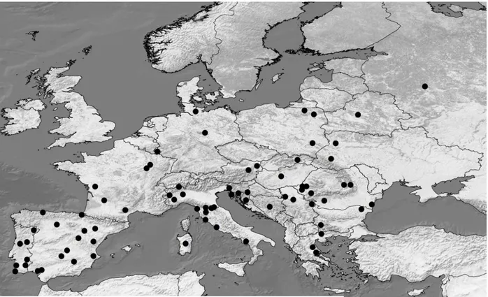
The dataset of 1099 sequences assembled includes sequences from three continents: Europe, Africa and Asia. In order to investigate the European history of the wild boar, only sequences of European origin were considerate. European sequences without spatial information were also discarded (samples from Finland and Belgium). Taking into account only European wild boars, a total of 763 sequences were obtained (467 newly sequenced, and 296 retrieved from previous published studies). These comprise 74 sampling sites from 19 countries (Figure 11).
38 Since the number of sequences per sample site varied from one to 83, samples with less than 10 individuals were grouped in further analysis. In so doing, haplotype composition of each population was taken into account, to avoid that populations with different colonization histories were joined. One population in Southern Italy (ISal), having n = 7 (after removal of three Asian haplotypes), was kept separated, as its allele composition was highly different from the nearest populations. After the grouping, a total of 39 populations were obtained (Figure 12).
The presence of Asian sequences in European wild boars is considered as a signal of hybridization with domestic pigs. Asian haplotypes belonging to clade A are present at a frequency as high as 29% in European domestic breeds (Fang & Andersson 2006). This is mainly due a historical introgression with Chinese domestic pigs during the 18-19th century (Giuffra et al. 2000). Given that four Asian haplotypes were found in the European wild boar (three in Italy and one in Luxembourg), in analysis involving the 39 populations or strictly wild boar samples, this four haplotypes were excluded since they come from a hybridization with domestic pigs, totaling 759 samples.