Facoltà di Ingegneria
Filomena Dato
A
N ITERATIVE MODEL FOR
V
ULNERABILITY
C
URVES
(
PGA
)
GENERATION OF MASONRY BUILDINGS
.
Tesi di Dottorato XXX ciclo Il Coordinatore
Prof. Ing. Luciano Rosati
Tutor
Prof. Arch. Giulio Zuccaro
Co-Tutor
Arch. Francesco Cacace Ing. Daniela De Gregorio
Dottorato di Ricerca in Ingegneria Strutturale, geotecnica e rischio sismico
On the front cover:
Vulnerability Curves of masonry buildings.
AN ITERATIVE MODEL FOR VULNERABILITY CURVES (PGA) GENERATION OF MASONRY BUILDINGS
__________________________________________________________________ Copyright © 2018 Università degli Studi di Napoli Federico II – P.le Tecchio 80, 80136 Napoli, Italy – web: www.unina.it
Proprietà letteraria, tutti i diritti riservati. La struttura ed il contenuto del presente volume non possono essere riprodotti, neppure parzialmente, salvo espressa autorizzazione. Non ne è altresì consentita la memorizzazione su qualsiasi supporto (magnetico, magnetico-ottico, ottico, cartaceo, etc.).
Benché l’autore abbia curato con la massima attenzione la preparazione del presente volume, Egli declina ogni responsabilità per possibili errori ed omissioni, nonché per eventuali danni dall’uso delle informazione ivi contenute.
To Enzo and Giuseppe
1
TABLE OF CONTENTS
Table of contents ... 1 List of Figures ... 3 List of Tables ... 9 Introduction ... 11 Summary ... 15 1 Seismic vulnerability ... 171.1 Seismic risk assessment ... 17
1.2 Buildings seismic vulnerability ... 21
1.2.1 Seismic hazard measures ... 23
1.2.2 Vulnerability classes ... 24
1.2.3 “SAVE” methodology... 25
1.2.4 The damage level ... 28
1.3 Seismic vulnerability assessment approaches ... 31
1.3.1 Observed vulnerability - Statistical approach. ... 32
1.3.2 Calculated Vulnerability - Mechanical approach. ... 34
1.3.3 Hybrid Method ... 35
1.4 Seismic vulnerability assessment tools ... 36
1.4.1 Damage Probability Matrices (DPM) ... 36
1.4.2 Vulnerability Index Method ... 40
1.4.3 Vulnerability Curves ... 42
2 The masonry structure ... 49
2.1 Introduction ... 49
2.2 Masonry structure ... 51
2.3 Mechanical models of masonry structure ... 54
2.4 The constitutive model ... 56
3 No-tension material (NTM) ... 59
3.1 The constitutive model of no-tension material. ... 62
3.1.1 Simplified uniaxial models ... 62
3.1.2 Approach formulated by G. Del Piero (1989) ... 64
3.1.3 Approach formulated by A. Baratta et al. (1991, 2005) .... 66
3.1.4 Approach formulated by D. Addessi et al. (2014) ... 69
4 Collapse mechanisms of masonry structures ... 73
4.1 Introduction ... 73
2
4.2.1 Elastic analysis ... 75
4.2.2 Limit analysis ... 75
4.3 Collapse mechanisms classification ... 77
4.4 Global collapse mechanisms ... 79
4.5 In-plane collapse mechanisms ... 81
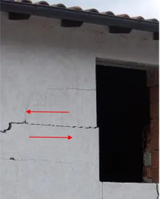
4.5.1 Shear crack ... 83
4.5.2 Failure by slip ... 88
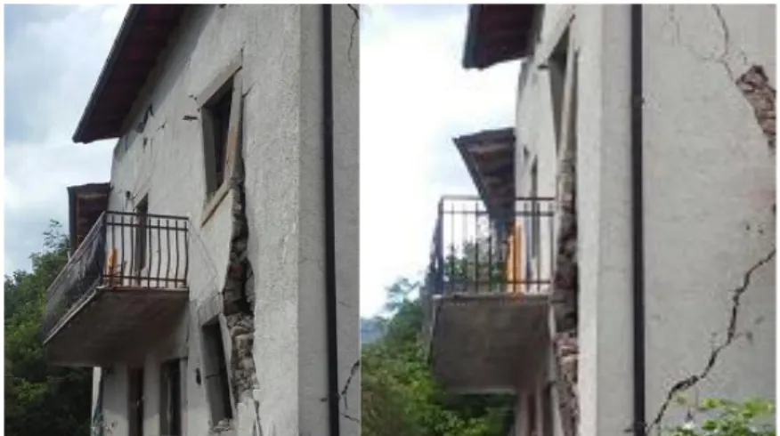
4.5.3 Buckling failure ... 91
4.6 Out-of-plane collapse mechanism ... 94
4.6.1 Simple overturning ... 97
4.6.2 Vertical bending ... 101
4.6.3 Horizontal bending ... 106
4.7 Analysis of the mechanisms of collapse: the case study of Fonte del Campo ... 112
4.7.1 Earthquake central Italy ... 112
4.7.2 Impact on the buildings ... 114
4.7.3 Analysis of Fonte del Campo ... 119
5 Research steps: the iterative model ... 133
5.1 Statistical analysis of existing masonry buildings ... 134
5.2 Iterative model generation. ... 136
5.3 Seismic Vulnerability classification by “SAVE” method. ... 138
5.4 Collapse Mechanisms calculation. ... 141
5.5 Vulnerability curves assessment ... 144
6 Research results: the vulnerability curves ... 145
6.1 Damage vulnerability curves... 150
6.2 Comparison with alternative strategies ... 152
7 Conclusions ... 161
3
LIST OF FIGURES
Fig. 1 The seismic activity map recorded by INGV National Seismic Network in 2016 (Iside, http://iside.rm.ingv.it). ... 17 Fig. 2 The seismic hazard map made by INGV National Seismic Network in 2016 (http://zonesismiche.mi.ingv.it/). ... 19 Fig. 3 Classification of structures (buildings) into vulnerability classes according to EMS 98 (Grünthal, 1998). ... 25 Fig. 4 Save Methodology (Zuccaro et al. 2006). ... 27 Fig. 5 Difference between SPDv function of EMS’98 and SPDP modified by vulnerability parameters. ... 27 Fig. 6 Classification of damage to masonry buildings according to EMS 98 (Grünthal, 1998). ... 29 Fig. 7 Classification of damage to buildings of reinforced concrete according to EMS 98 (Grünthal, 1998). ... 30 Fig. 8 The vulnerability assessment method; the bold path shows a traditional assessment method. (Calvi, 2006). ... 32 Fig. 9 Vulnerability functions to relate damage factor (d) and peak ground
acceleration (PGA) for different values of vulnerability index (IV ) (adapted
from Guagenti and Petrini(1989)) ... 42 Fig. 10 Lognormal cumulative distribution function. ... 44 Fig. 11 Vulnerability curves produced by Spence et al. (1992).D1 to D5 relate to damage states in the MSK scale... 45 Fig. 12 Simulated (thick line) and observed (thin line) vulnerability functions for MSK intensity VII (Barbat et al., 1996). ... 47 Fig. 13 Components of unreinforced brick (left) and unreinforced concrete block (right) walls. FEMA P-774 (2009). ... 49 Fig. 14 Reinforced brick wall (FEMA 1994). ... 50 Fig. 15 Breakdown of fatalities attributed to earthquake by cause (Period 1900-1999) Navaratnarajah, Sathiparan (2015). ... 51 Fig. 16 General classification of rubble masonry: (a) coursed masonry, (b) un-coursed masonry, (c) dry masonry, (d) “composite” masonry. ... 53 Fig. 17 General classification of ashlar masonry: (e) Fine masonry, (f) Rought masonry, (g) Chamfered masonry. ... 54
4
Fig. 18 Modeling method for masonry structures: (a) masonry sample, (b) detail micro-mechanical model, (c) simplified micro-mechanical model, (d) macro-mechanical model (Laurenҫo et al., 1995). ... 55 Fig. 19 Qualitative stress-strain diagram in uniaxial tension and compression (Ricamato et al, 2007). ... 56 Fig. 20 Stress - strain masonry curve (Ricamato et al, 2007). ... 57 Fig. 21 NTM model: yield surface in σx, σy, τxy stress space (Zuccaro and Papa, 1996)... 61 Fig. 22: (a) model zero, (b) model one, (c) model two, (Angelillo, 2014). .. 62 Fig. 23 No-tension plastic admissible stresses: normality rule of the fracture and crushing tensors. (D. Addessi, S. Marfia, E. Sacco and J. Toti , 2014) ... 72 Fig. 24 Typical earthquake damage of masonry structures due to different direction of shaking (Pitta, 2000)... 74 Fig. 25 MEDEA: Global Collapse Mechanisms (masonry). (Zuccaro et al. 2010). ... 78 Fig. 26 MEDEA: Local Collapse Mechanisms (masonry) (Zuccaro et al. 2010). ... 79 Fig. 27 Out-of-plane (left) and in-plane (right) behaviour of a single wall. ... 79 Fig. 28 In-plane collapse mechanisms: failure modes in unreinforced masonry walls (a ) Shear crack, (b) Failure by slip, (c) Buckling failure. . 81 Fig. 29 Macro-Element model of the masonry structure. ... 82 Fig. 30 Diagonal shear cracks due to earthquake Central Italy- Amatrice 2016. ... 84 Fig. 31 Diagonal shear cracks due to earthquake Central Italy- Arquata del Tronto 2016. ... 84 Fig. 32 Diagonal shear cracks due to earthquake Central Italy- Illica (Accumuoli) 2016... 85 Fig. 33 Shear crack mechanism ... 86 Fig. 34 Mohr’s circle for shear crack stress. ... 87 Fig. 35 Failure by slip due to earthquake Central Italy- Pescara del Tronto 2016. ... 89 Fig. 36 Failure by slip due to earthquake Central Italy- Illica (Accumuli) 2016. ... 90 Fig. 37 Failure by slip ... 90 Fig. 38 Buckling failure of a masonry wall ... 91
5
Fig. 39 Buckling failure due to earthquake Central Italy- Accumuli, 2016
... 92
Fig. 40 Buckling ultimate limit state ... 92
Fig. 41 Out-of-plane failure mechanisms of the FaMIVE method (D’Ayala and Speranza 2003) ... 95
Fig. 42 Simple overturning due to earthquake Central Italy, Accumuli, 2016 ... 98
Fig. 43 Vertical crack patterns between the wall and the orthogonal lateral walls, Illica, 2016 ... 98
Fig. 44 Simple overturning due to earthquake Central Italy, Amatrice, 2016 ... 99
Fig. 45 Simple overturning failure, vertical section of the wall ... 101
Fig. 46 Vertical bending of masonry wall due to earthquake Central Italy, Fonte del Campo, 2016. ... 102
Fig. 47 Vertical bending of masonry wall due to earthquake Central Italy, Illica, 2016 ... 102
Fig. 48 Vertical bending failure, vertical section of the wall ... 103
Fig. 49 Horizontal bending of a masonry wall (Borri, 2004) ... 107
Fig. 50 Horizontal bending due to earthquake Central Italy, Pescara del Tronto, 2016 ... 108
Fig. 51 Horizontal bending, horizontal section of the wall. ... 111
Fig. 52 Shake Map on 24 August in the Rieti, Ascoli and Perugia provinces. Source: INGV ... 112
Fig. 53 The seismic sequence started on 24th August in the Rieti, Ascoli and Perugia provinces (updated 16 September 2016). Source: INGV . 113 Fig. 54 Towns analysed by visual surveys on October 2016. ... 114
Fig. 55 Coursed rubble masonry, Illica October 2016. ... 115
Fig. 56 Un-coursed rubble masonry, Fonte del Campo October 2016 115 Fig. 57 Out-of-plane collapse mechanisms, Accumoli October 2016. . 116
Fig. 58 In-plane collapse mechanisms, Illica October 2016. ... 116
Fig. 59 Masonry building with RC roof, Accumoli October 2017. ... 117
Fig. 60 Masonry building renovated with mortar injection (on the left) and old collapsed masonry building (on the right), Saletta, October 2017. . 118
Fig. 61 Old masonry building with steel ties, Accumoli October 2017. 118 Fig. 62 Planimetry of Fonte del Campo. ... 119
Fig. 63 Classification of Fonte del Campo buildings. ... 120
Fig. 64 AeDes form: sections 3 and 4 ... 121
6
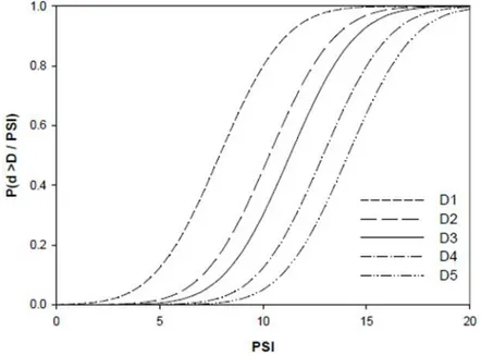
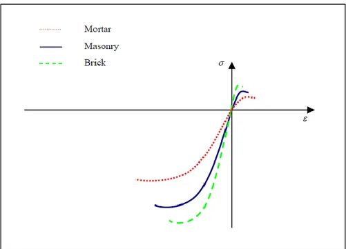
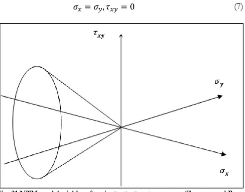
Fig. 66 Analysis of the Vulnerability class of the buildings of Fonte del Campo. ... 126 Fig. 67 Distribution of the Vulnerability classes of the buildings of Fonte del Campo. ... 127 Fig. 68 Levels of damage distribution on Fonte del Campo map. ... 128 Fig. 69 Damage state probability (D0, D1, D2, D3, D4, D5) observed on the vulnerability class of buildings of Fonte del Campo. ... 129 Fig. 70 Damage state probability observed for each mechanisms of collapse on the vulnerability classes of buildings of Fonte del Campo. 130 Fig. 71 Damage state probability observed for in-plane and out of plane mechanisms of collapse on the vulnerability classes of buildings of Fonte del Campo. ... 130 Fig. 72 Before and after the 24th August 2016 earthquake. Damage level 4 on vulnerability class A building in Fonte del Campo. ... 131 Fig. 73 Before and after the 24th August 2016 earthquake. Damage level 3 on vulnerability class B building in Fonte del Campo. ... 132 Fig. 74 Research methodology, Zuccaro at al. (2012). ... 133 Fig. 75 Earthquakes investigated in the Plinivs Study Centre Database. ... 135 Fig. 76 Lognormal distribution curves for buildings vulnerability class A as functions of trigger acceleration of each Collapse Mechanism (PGA) vs the Damage State probability ... 147 Fig. 77 Lognormal distribution curves for buildings vulnerability class B as functions of trigger acceleration of each Collapse Mechanism (PGA) vs the Damage State probability ... 148 Fig. 78 Lognormal distribution curves for buildings vulnerability class C as functions of trigger acceleration of each Collapse Mechanism (PGA) vs the Damage State probability ... 148 Fig. 79 Lognormal distribution curves for buildings vulnerability class D as functions of trigger acceleration of each Collapse Mechanism (PGA) vs the Damage State probability ... 149 Fig. 80 Mechanism type activating probability for each vulnerability class (A, B, C, D ... 150 Fig. 81 Damage Vulnerability Curves for each vulnerability Class (A, B, C, D). ... 151 Fig. 82 Damage Vulnerability Curves for each vulnerability Class (A, B, C, D). ... 152
7
Fig. 83 Comparison between damage Vulnerability Curves of vulnerability Class B and the one obtained by Cattari et al (2014) ... 153 Fig. 84 Comparison between damage Vulnerability Curves of vulnerability Class B and the one obtained by Cattari et al, 2014. ... 153 Fig. 85 Comparison between the In-plane mechanisms vulnerability curves and vulnerability curves derived from DPM [Zuccaro and De Gregorio, 2015] for vulnerability class A ... 155 Fig. 86 Comparison between the out of plane mechanisms vulnerability curves and vulnerability curves derived from DPM [Zuccaro and De Gregorio, 2015] for vulnerability class A ... 155 Fig. 87 Comparison between the In-plane mechanisms vulnerability curves and vulnerability curves derived from DPM [Zuccaro and De Gregorio, 2015] for vulnerability class B. ... 156 Fig. 88 Comparison between the out of plane mechanisms vulnerability curves and vulnerability curves derived from DPM [Zuccaro and De Gregorio, 2015] for vulnerability class B ... 156 Fig. 89 Comparison between the In-plane mechanisms vulnerability curves and vulnerability curves derived from DPM [Zuccaro and De Gregorio, 2015] for vulnerability class C ... 157 Fig. 90 Comparison between the out of plane mechanisms vulnerability curves and vulnerability curves derived from DPM [Zuccaro and De Gregorio, 2015] for vulnerability class C ... 158 Fig. 91 Comparison between the In-plane mechanisms vulnerability curves and vulnerability curves derived from DPM [Zuccaro and De Gregorio, 2015] for vulnerability class D ... 158 Fig. 92 Comparison between the out of plane mechanisms vulnerability curves and vulnerability curves derived from DPM [Zuccaro and De Gregorio, 2015] for vulnerability class D ... 159
9
LIST OF TABLES
Table 1 SPD range assigned for each vulnerability class of the buildings. ... 26 Table 2 Classification of damage according to the European Macroseismic Scale, EMS. ... 31 Table 3 Format of the Damage Probability Matrix Proposed by Whitman et al. (1973). ... 37 Table 4 Damage Probability Matrix, class A (Braga et al., 1982, 1985). . 37 Table 5 Damage Probability Matrix, class B (Braga et al., 1982, 1985). .. 38 Table 6 Damage Probability Matrix, class C (Braga et al., 1982, 1985)... 38 Table 7 DPM obtained through a statistical analysis of the data collected about the observed damages due to earthquakes occurred in Italy since 1980 (Zuccaro et al. , 2015). ... 39 Table 8 Typology of masonry components ... 51 Table 9 A sample of the information collected by AeDES and MEDEA forms. ... 123 Table 10 Typological characteristics identified on buildings of Fonte del Campo. ... 124 Table 11 A sample of the Seismic Vulnerability classification of the buildings of Fonte del Campo... 125 Table 12 Probability of combination between the typology of vertical structure of the buildings and other features (typology of horizontal structure, number of floors and percentage of openings). ... 135 Table 13 Main typological characteristics identified on existing masonry buildings and assigned to the virtual buildings by a random procedure. ... 136 Table 14 Dataset of virtual buildings generated by a random procedure. (Sample of the first 13 occurrences of the computed dataset). ... 137 Table 15 Seismic vulnerability classification of the virtual buildings (Sample of the first 13 occurrences of the computed dataset). ... 139 Table 16 Percentage of the virtual buildings, classified in vulnerability class buildings, calculated for each structural characteristics. ... 140 Table 17 Main typological characteristics identified on the virtual buildings classified in vulnerability classes. ... 141
10
Table 18 Value of the trigger acceleration (ag) corresponding to the
considered collapse mechanisms (sample of the first 8 occurrences of the computed dataset). ... 143 Table 19 Data computed in order to plot the normal distribution curves (arithmetic mean and standard deviation) and the lognormal distribution curves (logarithmic arithmetic mean and logarithmic standard deviation). ... 145
11
INTRODUCTION
In the last ten years, a large number of losses have been caused by earthquakes occurred in Italy (Abruzzo 2009, Emilia Romagna 2012, central Italy earthquake 2016). The collapse of masonry buildings is the primary cause for loss of life during an earthquake (Coburn & Spence, 2002), thus the strong interest to assess the seismic vulnerability of existing buildings to prepare seismic risk mitigation plans.
A good semantic definition of vulnerability is given by Sandi [1986]: “the seismic vulnerability of a building is its behaviour described by a cause-effect law, where the cause is the earthquake and the cause-effect is the damage”, however beside this a quantitative definition within the framework of the decision theory can be given: Vulnerability is the probability that an element at risk of a given typological class (i.e. A, B, C, ...) can accuse a level of damage (i.e. D1, D2, D3,…...) consequent to the action of a given level of hazard intensity (i.e. V, VI, VII,…….).
In order to perform vulnerability assessments of masonry buildings, several approaches, each one related to a different level of approximation, are available in the literature (Calvi et al., 2006). For the reader’s convenience, such strategies can be grouped in two categories:
• Observed vulnerability /Statistical approach.
The vulnerability is derived from the synthetic analysis of the formal and structural characteristics of the building.
A restricted number of building categories, called "vulnerability classes", are identified as a function of the typological and structural characteristics. Each class is then associated to an expected behaviour under seismic action, this behaviour is described by a vulnerability function that generally is calibrated by analyzing the damage observed during past events. Applications of this method, using the Damage Probability Matrices (DPM), were originally proposed by Whitman et al. (1973), who analyzed the damages observed in more than1600 buildings after the 1971 San Fernando earthquake, by Braga et al (1982,1986) after the 1980 south-Italia earthquake and by Zuccaro et al (2000), Bernardini et al (2007a, 2007b).
12
The validity of this approach is reliable on a large number of buildings having characteristics to be included in specific vulnerability classes, obviously it is not reliable for single buildings. On the other hand it has the undeniable advantage of demanding both little information and rapid processing. Furthermore, it is derived from observations of the actual performance of assets in real earthquakes. For this reason it is useful for investigating a wide range of buildings (urban scale or wider). The research in this context aims to achieve a greater reliability of results while maintaining an acceptable agility of the investigation.
• Calculated Vulnerability/ Mechanical approach.
The vulnerability evaluation is the result of accurate computations using simplified limit state analysis on predefined categories of Structural Mechanics.
The damage evaluation is formulated on the basis of analytical calculations to determine the seismic response of the building, the stress and corresponding strain state are derived.
In this way, the problem of seismic vulnerability of masonry structures is developed in structural engineering terms. Vulnerability is computed as a direct function of construction characteristics, structural response to seismic actions and damage effects. Applications of this method can be seen in the work of Giuffrè (1991), Singhal and Kiremidjian (1996), Park and Ang (1985), Masi (2003), Rossetto and Elnashai (2005), Dumova-Jovanoska (2004), D’Ayala et al. (2015).
This approach provides assessments certainly more reliable on single buildings, but it requires detailed knowledge of technical features of the buildings and the development of time consuming structural calculations. Therefore it is difficult to implement at large scale.
Despite its robustness, the mechanical approach requires a detailed knowledge of structural features of the analyzed buildings and high computational efforts in computing the structural responses and, for these reasons, it is hardly implemented at a large scale.
In order to overcome the drawbacks of both these strategies, hybrid methodologies, aiming at combining the results of a simplified mechanical model with the vulnerability evaluations of a statistical approach, have been recently proposed. Their main philosophy consists in enriching a limited dataset, which is statistically analyzed, by the computation of
13
simulated mechanical data or, alternatively, to introduce probabilistic corrections, derived by observed dataset, in a mechanical model, see, e.g., Cavalieri et al. (2017).
Following a hybrid approach, the procedure presented in this dissertation aims to develop collapse probability distribution for a set of building classes suitable for the Italian structural typologies. In particular, the statistical data derived by the survey of about 250,000 buildings is adopted to randomly generate a virtual set of mechanical models where each instance is characterized by mechanical properties relevant to a typological class according to the vulnerability assessment method proposed by Zuccaro et al. (2012). The structural models are analyzed by means of simplified limit state analysis procedures in order to evaluate their seismic response and to compute the vulnerability probability curves, expressed in terms of seismic acceleration for each typological class.
In particular, the adopted hybrid methodology, aiming to determine the vulnerability curves as functions of the structural typology and of the seismic acceleration, can be described in the following steps both statistical and mechanical nature:
i. Statistical analysis of existing masonry buildings. The analysis, pursued
thanks to the PLINIVS Study Centre1 Database, is based on the
survey performed all along the Italian peninsula. About 250,000 of the residential masonry buildings (ISTAT Census 2011) have been surveyed distributed on about 600 municipalities. This analysis has allowed to investigate the geometrical and structural characteristics of Italian masonry buildings and identify the recurring combinations of these characteristics. The probability of combination between a particular characteristic (e.g. type of vertical structure) and other features (e.g. type of horizontal structure, presence of ties, etc.) have been then evaluated.
ii. Iterative model generation. An iterative procedure has been
implemented by an ad-hoc software developed in order to generate virtual model of buildings (about 100,000). The program adopts a random assignment procedure of the structural
1 PLINIVS Study Centre for Hydrogeological, Volcanic and Seismic Engineering.
University of Naples, Italy. Centre of competence of Italian Civil Protection. www.plinivs.it
14
characteristics whose probability distributions are known from previous step.
iii. Seismic Vulnerability classification by “SAVE” method2. The generated
virtual buildings have been classified in vulnerability classes (A, B, C, D) according to the assignment procedure based on the criteria defined in the "SAVE" project (Zuccaro et al. 2015).
iv. Collapse Mechanisms calculation. For each virtual building the trigger
acceleration (ag) responsible of the relevant Collapse Mechanisms have been computed. The mechanisms considered, assumed with reference to the classification adopted in the MEDEA methodology (Zuccaro and Papa, 2002), are: in-plane (shear crack, failure by slip and buckling failure) and out-of-plane (simple overturning, vertical bending and horizontal bending) collapse mechanisms.
iv. Vulnerability curves assessment. Collecting the obtained results, for
each typological class (A, B, C, D), vulnerability curves are built, expressing the collapse probability as a function of the ground acceleration (ag ).
The approach adopted constitutes a preliminary study to understand the basic seismic behaviour of the ordinary masonry buildings. Further developments of this research will include additional improvements also in dynamic state, able to identify a more accurate evaluation of collapse accelerations (Boothby, 2001; De Jong, 2009), considering micromechanical modelling of failure (effects of deformations in the mortar joints, detailed properties of the material, irregularity in the panels, etc.) and more detailed sensitivity analyses on the observed data used and on their reliability.
2 “SAVE” - Updated Tools for the Seismic Vulnerability Evaluation of the Italian Real
15
SUMMARY
This dissertation includes a detailed analysis of the seismic vulnerability assessment of the masonry buildings. Chapter 1 starts from the definition of the seismic risk assessment and reviews the relevant literature for the buildings seismic vulnerability assessment. In particular, this study discusses the current state of the buildings seismic vulnerability approaches (observed vulnerability, calculated vulnerability and hybrid approach) and their assessment tools (damage probability matrices, vulnerability index method, vulnerability curves).
Moreover Chapter 2 includes details about the mechanical characteristics of the masonry structure and its constitutive models. Chapter 3 includes an analysis of the no-tension material (NTM) according to Heyman (Heyman, 1966; Heyman, 1969) assumptions. In particular the chapter reviews some formulations of the constitutive problem of no-tension material, all based on the use of mathematical algorithmic (Del Piero (1989), Baratta et al. (1991, 2005), Addessi (2014)).
Chapter 4 analysed the collapse mechanisms (in-plane and out-of-plane) potentially triggered in masonry buildings by the seismic action. This work, based on Heyman's general principles of limit analysis (Heyman 1966, 1995, 1998), examines the collapse mechanisms of masonry structures in response to horizontal ground accelerations. The masonry structure is analyzed using rigid block or “macro-elements” analysis based on equilibrium and making work calculations in order to verify the stability of the structure and determine the critical collapse mechanism. In particular in paragraph 8.7 the study of the mechanisms of collapse is used to analyze the seismic damage caused by the earthquake that hit the central Apennines on 24th August, 2016. In particular, among all towns, it is investigated the case study of Fonte del Campo.
The hybrid vulnerability approach presented in this dissertation is analysed in Chapter 5, which also summarizes the iterative procedure adopted in this research based on a Montecarlo simulation analysis.
Numerical results are presented by discussing the failure probability curves relevant to each collapse mechanism, and by computing the vulnerability curves of each structural typology, shown in Chapter 6.
16
The presented results are compared with alternative strategies, such as the approach proposed by Cattari et al., (2014) and the procedure presented by Zuccaro et al. (2015). A brief discussion on such comparisons and on the robustness of the proposed algorithm is reported in paragraph 6.2; Finally, conclusions and future work are summarized in Chapter 7.
17
1 SEISMIC VULNERABILITY
1.1 S
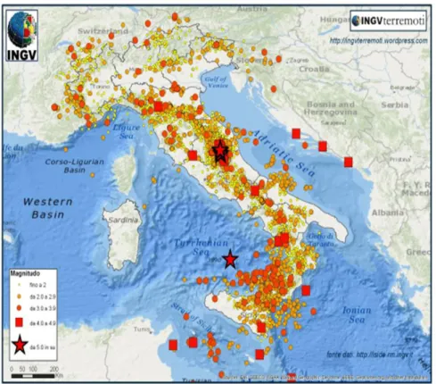
EISMIC RISK ASSESSMENTEvery year, from 1700 to 2500 earthquakes equal to or greater than
magnitude 2.5 occurred in Italy (INGV database) (Fig. 1). These
earthquakes range from very small events felt by only a few individuals to great earthquakes that destroy entire cities.
Fig. 1 The seismic activity map recorded by INGV National Seismic Network in 2016 (Iside, http://iside.rm.ingv.it).
The number of lives, lost and the amount of economic losses that result from an earthquake depend on the size, depth and location of the earthquake, the intensity of the ground shaking and related effects on the
18
building inventory, and the vulnerability of that building inventory to damage.
The seismic risk assessment has a fundamental role for the society because provides all the information for each community or organizations to support the risk mitigation decision-making.
The seismic risk can generally be defined as the measurement of the damage expected in a given interval of time, based on the type of seismicity, the resistance of buildings and the nature, quality and quantity of assets exposed.
The seismic risk is determined by the convolution of three parameters: hazard, exposure and vulnerability. They can be defined as:
Seismic hazard is defined as the probability in a given area and in
a certain interval of time of an earthquake occurring that exceeds a certain threshold of intensity, magnitude or peak ground acceleration (PGA).
It can be evaluated from instrumental, historical, and geological observations and is quantified by two parameters: a level of hazard and its recurrence interval or frequency: for example, an M7.5 earthquake with a recurrence interval of 500 years, and peak ground acceleration (PGA) of 0.3g with a return period of 1,000 years.
Two major approaches – deterministic and probabilistic – are worldwide used at present for seismic hazard assessment.
The deterministic approach is based on the study of damage observed during seismic events in the past at a given site, reconstructing the damage scenarios to determine the frequency of repetition of earthquakes of the same intensity.
In the probabilistic approach, initiated with the work of Cornell (1968), the seismic hazard is estimated in terms of a ground motion parameter – macroseismic intensity, peak ground acceleration – and its annual probability of return period at a site. The method yields regional seismic probability maps, displaying contours of maximum ground motion (macroseismic intensity, PGA) of equal – specified – return period.
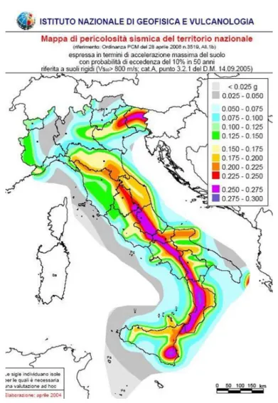
In Italy there are numerous studies and documents regarding the seismic hazard of the peninsula, representing by a seismic hazard
19
Fig. 2 The seismic hazard map made by INGV National Seismic Network in 2016 (http://zonesismiche.mi.ingv.it/).
It is clear that although seismic hazard and risk have often been used interchangeably, they are fundamentally different concepts. High seismic hazard does not necessarily mean high seismic risk, and vice versa. For example, there are high seismic hazards in the California deserts, but low seismic risk because there are few exposures (people or buildings).
20
In a seismic risk assessment the exposure is defined as a quality
and quantity analysis of assets (people, buildings, infrastructure and activities) exposed. The first objective for a general risk mitigation project is safeguarding human life. For this reason it is very important to assess the number of people involved, dead and/or injured using calculations based on the number of collapsed or damaged buildings.
Seismic vulnerability can be defined as the probability that exposed
assets (people, buildings, infrastructure and activities) have a given level of damage due to a seismic event of a given intensity. One of the main causes of death during an earthquake is building collapse. The kind of building damage depends on: the duration and intensity of the earthquake, the structure of the building, its age, materials, location, vicinity to other buildings and non-structural elements.
In order to estimate seismic risk, we have to assume a model (distribution) for the probability of earthquake occurrence in time. One commonly used distribution is the Poisson model (Cornell, 1968).
The methodology of the risk analysis, including hazard, vulnerability and exposed assets, depends on the geographical scale of the task (national scale, regional scale or local studies of urban areas).
The studies on the Italian peninsula show that Italy has high seismic risk, in terms of victims, damage to buildings and direct and indirect costs expected after an earthquake. It has a medium-high seismic hazard (due to the frequency and intensity of phenomena), very high vulnerability (due to the fragility of building, infrastructural, industrial, production and service assets) and an extremely high exposure (due to population density and its historical, artistic and monumental heritage that is one of its kind in the world).
In order to reduce the seismic risk, it is useful to reduce the vulnerability of the exposed assets.
Most of the loss of lives and casualties during an earthquake are caused by the collapse of structures and buildings thus it is fundamental to assess the seismic vulnerability status of existing buildings and include the results of this assessment in the planning of seismic risk mitigation.
21
This study includes a detailed analysis of the seismic vulnerability of the buildings and its assessment methodologies.
1.2 B
UILDINGS SEISMIC VULNERABILITYThe seismic vulnerability in the study is considered exclusively in the structural sense, implying the ability of buildings and structures to resist damage from earthquakes.
A good definition of vulnerability is given by Sandi (1986): “the seismic vulnerability of a building is its behavior described by a cause- effect law, where the cause is the earthquake and the effect is the damage”.
There are different factors that affect the overall vulnerability of a structure besides construction type. These factors, described by Grünthal (1998) in EMS 98, are generally applicable to all types of structures:
Quality of the materials and workmanship.
A building that is well-built will be stronger than one that is badly built. The use of good quality materials and good construction techniques is crucial to improving the seismic behavior of the building. In the case of materials, the quality of the mortar is particularly important, and even rubble masonry can produce a reasonably strong building if the mortar is of high quality. Poor workmanship can include both carelessness and cost-cutting measures, such as a failure to tie in properly parts of the structure. In cases of poorly built engineered structures, it may be that the finished structure actually fails to meet the provisions of the appropriate seismic building code.
State of preservation and strengthening of the buildings.
A good state of preservation allows to have a performance of the building in accordance with its expected strength from other factors. A building which has been allowed to decay may be significantly weaker. In cases of abandoned or derelict buildings, and also in cases where there is an evident lack of maintenance some measures must been taken to retrofit buildings in order to improve their seismic behaviour.
22
It is often possible to observe in damaged buildings how the irregularity contributed to the bad seismic behavior. The ideal building would be a cube in which all internal variations in stiffness (like stairwells) were symmetrically arranged. Regularity should be considered in a global sense in plan and elevation. In some cases, especially old masonry buildings, buildings that previously had a good level of regularity may be adversely affected by subsequent modifications
Ductility.
Ductility is defined as the ability of the structure or parts of it to sustain large deformations beyond the yield point without breaking. It depending on the construction type and structural system. In the field of applied seismic engineering, the ductility is expressed in terms of demand and availability. The ductility demand is the maximum ductility level that the structure can reach during a seismic action, which is a function of both the structure and the earthquake. The available ductility is the maximum ductility that the structure can sustain without damage and it is an ability of the structure. In buildings designed against earthquakes, the parameters of the building determining dynamic characteristics will be controlled.
Position of the building.
The position of a building with respect to other buildings in the vicinity can affect its behavior in an earthquake. In the case of a houses anchored to a neighbor causing an irregularity in the overall stiffness of the structure which will lead to increased damage. Severe damage can be the result of two tall buildings of different natural periods that are situated too close to one another. During an earthquake they may sway at different frequencies and smash into each other, causing an effect known as pounding.
The aim of a vulnerability assessment is to obtain the probability of a specific level of damage caused by a scenario earthquake to a given building type.
In order to assess a seismic vulnerability of an urban area it is not always possible to analyze the characteristics of each single building. It is recommended to group the buildings that have similar seismic behavior in typological classes also known as vulnerability buildings classes.
23
In summary, a seismic vulnerability assessment take in to account three elements:
i. The measures of the earthquake.
ii. The vulnerability class of the buildings.
iii. The damage level.
1.2.1 Seismic hazard measures
A vulnerability assessment needs a particular characterization of the ground motion, which will represent the seismic demand of the earthquake on the building.
Traditionally, the measures of the earthquake is expressed in macroseismic intensity scales (Modified Mercalli Intensity, MMI, EMS 98) and instrumental quantities (peak ground acceleration, PGA).
Macroseismic intensity scales are based on how strongly the ground shaking is experienced in an area, as well as observations of building damage. This means that macroseismic scales include information about building fragility in the areas in which they have been calibrated. This should be taken into account when applying a macroseismic scale outside the area in which it was originally developed – for example, using the European Macroseismic Scale (EMS) outside Europe.
The Macroseismic intensity scales have this characteristics:
They are discrete rather than continuous and often Roman
numerals are used to reflect this.
They are monotonic (in the sense that VII generally relates to a
stronger ground shaking than VI, for example), but nonlinear (each increment does not necessarily represent a constant increase in ground shaking).
Instrumental intensity measures are based on quantities that are calculated from strong ground motion recordings. The most commonly used instrumental measure in the vulnerability literature is peak ground acceleration (PGA). Compared with macroseismic scales, instrumental measures may be less correlated with damage.
More recent proposals have linked the seismic vulnerability of the buildings to response spectra obtained from the ground motions.
24
1.2.2 Vulnerability classes
A vulnerability classes express a different ways that buildings respond to earthquake shaking.
Grünthal (1998) gives a general description of the vulnerability class: “If two groups of buildings are subjected to exactly the same earthquake shaking, and one group performs better than the other, then it can be said that the buildings that were less damaged had lower earthquake vulnerability than the ones that were more damaged, or it can be stated that the buildings that were less damaged are more earthquake resistant, and vice versa”.
The most common scale used to classify the buildings vulnerability is the EMS scale (Grünthal, 1998).
The EMS 98 defined four groups of buildings structure (masonry, RC,
steel and wood) and six classes of decreasing vulnerability (A-F) (Fig. 3):
The A, B and C classes represent the strength of an adobe house, brick building and reinforced concrete (RC) structure. They should be compatible with building classes A-C in the MSK-64 and MSK-81 scales. Classes D and E are intended to represent an improved level of earthquake resistant buildings as reinforced or confined masonry and steel structures, which are well-known to be resistant to earthquake shaking. Class F is intended to represent the vulnerability of a structure with a high level of earthquake resistant design.
25
Fig. 3 Classification of structures (buildings) into vulnerability classes according to EMS 98 (Grünthal, 1998).
In some cases, the EMS 98 vulnerability scale has high level of uncertainty: the “probable range” may be large and this can falsify the planning of seismic risk mitigation.
1.2.3 “SAVE” methodology
Zuccaro et al. (2006, 2009, 2015) made a reformulation of EMS 98 vulnerability classes assignment. This procedure, defined as “SAVE” methodology (Strumenti di Analisi di Vulnerabilità degli Edifici esistenti), classifies the buildings taking into account not only the vertical structure of the buildings as in EMS 98 but also the typological-structural characteristics of the buildings or "vulnerability factors".
26
The vulnerability factors are defined as the most recurrent structural characteristics responsible of the seismic behavior of the buildings (pushing roofs, floor stiffness etc.).
This typological characteristics are identified through the analysis of the observed damages due to previous earthquakes and parameterized through the Synthetic Parameter of Damage (SPD).
The SAVE assignment procedure can be synthetically defined in these
steps (Fig. 4):
i. Each building is classify according to EMS 98 vulnerability scale.
ii. The SPDv is obtained calculating the average value of SPD
corresponding to the EMS 98 class of the building. The table (Table 1) shows the range of SPD values assigned for each
vulnerability class of the buildings. The values of the SPD range is the result of a statistical analysis of the average behavior of buildings with same characteristics.
Table 1 SPD range assigned for each vulnerability class of the buildings.
Vulnerability class
A B C D E
- 2.0 1.7 1.4 1.0
2.0 1.7 1.4 1.0 -
iii. The typological-structural characteristics of the building
(vulnerability factors) are analysed and parameterized in coefficients of influence (positive or negative) “Ps(1,2,3…)”.
iv. The results thus obtained is summed with the value of the SPDv
to obtain a new value defined as SPDP. If the SPDP is bigger than SPDv this means that the building structure has a lower resistance
than that evaluated by the EMS 98 and vice versa (Fig. 5).
v. A new vulnerability class, corresponding to the value of SPDP, is
27
Fig. 4 Save Methodology (Zuccaro et al. 2006).
Fig. 5 Difference between SPDv function of EMS’98 and SPDP modified by vulnerability parameters.
28
1.2.4 The damage level
Each vulnerability assessment method models the level of damage on a discrete damage scale according to the MSK scale (Medvedev and Sponheuer, 1969), the Modified Mercalli scale (Wood and Neumann, 1931) or the EMS98 scale (Grünthal, 1998).
The most frequently used method is the classification according to European Macroseismic Scale (EMS) 1998, which includes a low level of damage (Level 0, Level 1, Level 2), a substantial to heavy damage state (Level 3), very heavy damage state (Level 4), and destruction damage state (Level 5).
The way in which a building deforms under earthquake shaking depends on the building type.
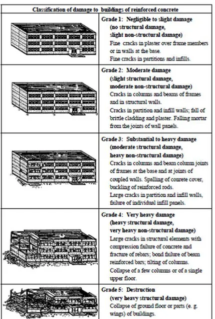
EMS 98 analyzed the classification of damage in two categories: masonry
buildings (Fig. 6) and buildings of reinforced concrete (Fig. 7).
In both categorizes is it possible to distingue the damage to the primary (load bearing/ structural) system and damage to secondary (non-structural) elements (like infill or curtain walls).
29
Fig. 6 Classification of damage to masonry buildings according to EMS 98 (Grünthal, 1998).
30
Fig. 7 Classification of damage to buildings of reinforced concrete according to EMS 98 (Grünthal, 1998).
In summary, the table (Table 2) shows the general descriptions of damage
31
Table 2 Classification of damage according to the European Macroseismic Scale, EMS. Damage Level Description D0 No damage D1 Cracking of non-structural elements, such as dry walls. Brick or stucco external cladding
D2
Major damage to the non- structural elements, such as collapse of a whole masonry infill wall; minor damage to load bearing elements D3 Significant damage to load-bearing elements, but no
collapse
D4 Partial structural collapse (individual floor or portion of building)
D5 Full collapse
1.3
S
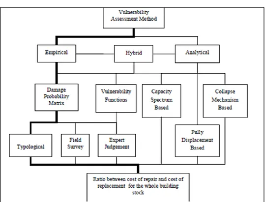
EISMIC VULNERABILITY ASSESSMENT APPROACHESThe various approaches for vulnerability assessment that have been proposed in the last 30 years and used in loss estimation can be divided into two main categories: statistical or empirical approach and mechanical or analytical approach, both of which can be used in hybrid approaches. (Fig. 8).
The choice of the most suitable procedure is highly dependent on the resources available and the scale and aim of the study. Statistical approach can be used for large scale studies to define damage scenarios, however if the purpose of the study is to identify within a district or urban center specific buildings in need of strengthening, so as to increase their seismic resilience, then a suitable mechanical procedure should be preferred.
32
Fig. 8 The vulnerability assessment method; the bold path shows a traditional assessment method. (Calvi, 2006).
1.3.1 Observed vulnerability - Statistical approach.
This method constitutes the only reasonable and possible approach that could be initially employed in seismic risk analyses at a large scale.
It has been first carried out in the early 70’s and calibrated as a function of macroseismic intensities. Applications of this method, using the Damage Probability Matrices (DPM), were originally proposed by Whitman et al. (1973), who analyzed the damages observed in more than 1600 buildings after the 1971 San Fernando earthquake, by Braga et al (1982,1986) after the 1980 south-Italia earthquake and by Zuccaro et al (2000), Bernardini et al (2007a, 2007b).
33
The statistical assessment method classify the vulnerability of the buildings based on damage observed in previous earthquakes to the same kind of buildings.
This method is generally the most desirable from a risk management viewpoint because it is derived wholly from observations of the actual performance of assets in real earthquakes.
Although this method is an observational method and hence of good affability, in practice there are several uncertainties about the way in which the data are acquired.
To produce such statistical analysis, large sets of data are needed to cover the whole range of performances of a given building typology to the whole range of possible seismic intensity considered, and multiple observations of building performance for the same level of intensity.
However, it has been seen that is not always possible to require damage data from past earthquakes and that the damage data available today are inadequate, especially for intensities greater than MMVII.
In general, any procedure for the statistical prediction of damage consists basically of three steps: collecting observations after an earthquake, grouping the results by buildings characteristics and performing a statistical analysis of the data.
First the observations of previous earthquakes are collected recording: xi = intensity of the earthquake at each building i
yi = damage of the building i
ci = attributes of the building i (structural material, lateral force resisting system, height, age, etc.)
Second the results are analyzed and grouped by one or more attributes of the buildings or by vulnerability classes of the building. A last, for each group of the data a statistical analysis (average, standard deviation, regression analysis…) is made.
There are three main types of statistical tools using in statistical approach for the seismic vulnerability assessment of buildings: damage probability matrices (DPM), Vulnerability Index Method and vulnerability functions.
34
1.3.2 Calculated Vulnerability - Mechanical approach.
The mechanical approach determines the response of a particular building, representative of a typology, by using structural analysis techniques and numerical tools. Applications of this method can be seen in the work of Giuffrè (1991), Singhal and Kiremidjian (1996), Park and Ang (1985), Masi (2003), Rossetto and Elnashai (2005), Dumova-Jovanoska (2004), D’Ayala et al. (2015).
This approach is particularly useful when studying a single building or a single typology of building or when assessing the improved performance due to strengthening and retrofit.
The reliability of the results is affected by the simulated models that reproduce the main characteristics of the buildings and their structural behavior. It is also dependent on the numerical tools available and by the ability of the assessor to interpret the results.
Mechanical methods, which use numerical simulations to analyze the structural behavior of buildings, are more sophisticated approaches than statistical methods. The data required for these approaches can be extracted from construction drawings and/or laboratory tests.
These approaches present the advantage of framing the problem of seismic vulnerability of masonry structures in structural engineering terms, defining their vulnerability as a direct function of construction characteristics, structural response to seismic actions and damage effects. However the following should be noted in applying these methods: • Mechanical methods are suitable to identify structural damage states, through structural analysis. They are less useful in quantifying the likely damage to content and non-structural elements.
• Many of the different mechanical approaches that exist are specific to particular types of structure, and have diverse data requirements and computational burdens.
• When comparing results from different mechanical methods it should be borne in mind that output in terms of vulnerability are dependent on different assumptions on the representative intensity measures chosen and representative response measures chosen.
According to "Norme Tecniche per le Costruzioni" (DM 14-1-2008) mechanical methods used to predict the seismic performance of a building are:
Linear static analysis.
35
Nonlinear static analysis. (Pushover analysis)
Nonlinear dynamic analysis (NDA).
The last two are considered the most accurate methods for predicting Reinforced Concrete building response to earthquake ground motion. The most used seismic analysis of unreinforced masonry structures is based on mechanical approach. Mechanical method is based on the application of kinematics models, which identify lateral collapse load multipliers of a given configuration of macro-elements and loads by imposing either energy balance or equilibrium equations. These methods present the advantage of requiring few input parameters to estimate the vulnerability and to identify the occurrence of possible in-plane or out of plane mechanisms for a given building.
1.3.3 Hybrid Method
Hybrid methods combine post-earthquake damage statistics with simulated, analytical damage statistics from a mathematical model of the building typology. Applications of this method can be seen in the work of Kappos et al. (1995, 1998), Barbat et al. (1996), Zuccaro et al. (2012), Cavalieri et al. (2017).
These methods are useful when there is a lack of damage data at certain intensity levels for the geographical area under consideration and they also allow calibration of the analytical methods.
Kappos et al. (1995, 1998) have derived damage probability matrices using a hybrid procedure. The DPMs for each intensity level were constructed using the available data from past earthquakes and the results of nonlinear dynamic analysis of models that simulated the behaviour of each building class. Intensity and PGA were correlated using empirical relationships. Barbat et al. (1996) made a hybrid vulnerability assessment of Spanish urban areas. A post-earthquake study was initially performed for two earthquakes with a maximum intensity of VII on the MSK scale.
Statistical analyses were then performed to obtain the vulnerability function for the MSK intensity level VII. A computer simulation process was subsequently used to obtain the vulnerability functions at other intensity levels.
The main difficulty in the use of hybrid methods is that the two vulnerability curves, statistical and mechanical, include different sources
36
of uncertainty and are thus not directly comparable. In the mechanical curves the sources of uncertainty are clearly defined during the generation of the curves whilst the specific sources and levels of variability in the statistical data are not quantifiable. The method used to calibrate the mechanical vulnerability curves using statistical data should include the additional uncertainty present in the statistical data which is not accounted for in the mechanical data.
1.4 S
EISMIC VULNERABILITY ASSESSMENT TOOLSRegardless of the assessment method used, there are three main types of statistical tools using for the seismic vulnerability assessment of buildings: damage probability matrices (DPM), Vulnerability Index Method and vulnerability functions.
1.4.1 Damage Probability Matrices (DPM)
The Damage Probability Matrices (DPM), traditionally derived using observed damage data, express in a discrete form the probability that a building obtaining a damage level j, due to a ground motion of intensity i (1):
P [D = j| i] (1)
The concept of a DPM is that a given structural typology will have the same probability of being in a given damage state for a given earthquake intensity.
The general form of DPM suggested by Whitman et al. (1973) is compiled for various structural typologies according to the damaged sustained in
over 1600 buildings after the 1971 San Fernando earthquake (Table 3).
Damage to buildings is described by a series of damage states (DS), while the intensity of the earthquake is described by the modified Mercalli intensity (MMI) scale. In a particular column, each number PDSI in the matrix is the probability that a particular state of damage will occur, given that a level of earthquake intensity is experienced. The sum of the probabilities in each column is 100%.
37
Table 3 Format of the Damage Probability Matrix Proposed by Whitman et al. (1973).
Damage
State Structural Damage
Non- Structural Damage Damage Ratio (%) Intensity of Earthquake V VI VII VIII IX 0 None None 0-0.05 95 79 33 6 0 1 None Minor 0.05-0.3 5 18 34 19 2 2 None Localized 0.3-1.25 0 3 20 44 18 3 Not Noticeable Widespread 1.25-3.5 0 0 10 13 30 4 Minor Substantial 3.5-7.5 0 0 3 6 20 5 Substantial Extensive 7.5-20 0 0 0 12 10 6 Major Nearly Total 20-65 0 0 0 0 7 7 Building Condemned 100 0 0 0 0 8 8 Collapse 100 0 0 0 0 5
One of the first European versions of a damage probability matrix was
produced by Braga et al. (1982) (Table 4, Table 5, Table 6), which was based
on the damage data of Italian buildings after the 1980 Irpinia earthquake. The damage distributions of any class buildings for different seismic intensities was described by a binomial distribution which has the advantage of needing one parameter only which ranges between 0 and 1. The buildings were separated into three vulnerability classes (A, B and C) and a DPM based on the MSK scale was evaluated for each class.
Table 4 Damage Probability Matrix, class A (Braga et al., 1982, 1985). Class A
Intensity of
Earthquake 0 1 2 Damage State 3 4 5
VI 0.188 0.373 0.296 0.117 0.023 0.002
VII 0.064 0.234 0.344 0.252 0.092 0.014
VIII 0.002 0.020 0.108 0.287 0.381 0.202
IX 0.0 0.001 0.017 0.111 0.372 0.489
38
Table 5 Damage Probability Matrix, class B (Braga et al., 1982, 1985). Class B
Intensity of
Earthquake 0 1 Damage State 2 3 4 5
VI 0.36 0.408 0.185 0.042 0.005 0.0
VII 0.188 0.373 0.296 0.117 0.023 0.002
VIII 0.031 0.155 0.312 0.313 0.157 0.032
IX 0.002 0.022 0.114 0.293 0.376 0.193
X 0.0 0.001 0.017 0.111 0.372 0.498
Table 6 Damage Probability Matrix, class C (Braga et al., 1982, 1985). Class C
Intensity of
Earthquake 0 1 2 Damage State 3 4 5
VI 0.715 0.248 0.035 0.002 0.0 0.0
VII 0.401 0.402 0.161 0.032 0.003 0.0
VIII 0.131 0.329 0.330 0.165 0.041 0.004
IX 0.050 0.206 0.337 0.276 0.113 0.018
X 0.005 0.049 0.181 0.336 0.312 0.116
Later, an additional vulnerability class D has been included, using the EMS98 scale (Grüntal, 1998), to account for the buildings that have been constructed since 1980. These buildings should have a lower vulnerability as they have either been retrofitted or designed to comply with recent seismic codes.
An example of Damage Probability Matrices (DPM) which take in to
account the EMS98 scale are exposed by Zuccaro et al. (2015) (Table 7)
The DPM are obtained by a statistical analysis, made thanks to the PLINIVS Study Centre Database, which is based on the data collected on the observed damages due to previous earthquakes taken place in Italy since 1980.
About 4% of the 6.903.982 residential masonry Italian buildings (ISTAT 2011) belonging to about 550 municipalities was investigated.
39
Table 7 DPM obtained through a statistical analysis of the data collected about the observed damages due to earthquakes occurred in Italy since 1980 (Zuccaro et al. , 2015).
Class Intensity of Earthquake
Damage State D0 D1 D2 D3 D4 D5 A V 0,3487 0,4089 0,1919 0,0450 0,0053 0,0002 B 0,5277 0,3598 0,0981 0,0134 0,0009 0,0000 C 0,6591 0,2866 0,0498 0,0043 0,0002 0,0000 D 0,8587 0,1328 0,0082 0,0003 0,0000 0,0000 A VI 0,2887 0,4072 0,2297 0,0648 0,0091 0,0005 B 0,4437 0,3915 0,1382 0,0244 0,0022 0,0001 C 0,5905 0,3281 0,0729 0,0081 0,0005 0,0000 D 0,7738 0,2036 0,0214 0,0011 0,0000 0,0000 A VII 0,1935 0,3762 0,2926 0,1138 0,0221 0,0017 B 0,3487 0,4089 0,1919 0,0450 0,0053 0,0002 C 0,5277 0,3598 0,0981 0,0134 0,0009 0,0000 D 0,6591 0,2866 0,0498 0,0043 0,0002 0,0000 A VIII 0,0656 0,2376 0,3442 0,2492 0,0902 0,0131 B 0,2219 0,3898 0,2739 0,0962 0,0169 0,0012 C 0,4182 0,3983 0,1517 0,0289 0,0028 0,0001 D 0,5584 0,3451 0,0853 0,0105 0,0007 0,0000 A IX 0,0102 0,0768 0,2304 0,3456 0,2592 0,0778 B 0,1074 0,3020 0,3397 0,1911 0,0537 0,0060 C 0,3077 0,4090 0,2174 0,0578 0,0077 0,0004 D 0,4437 0,3915 0,1382 0,0244 0,0022 0,0001 A X 0,0017 0,0221 0,1138 0,2926 0,3762 0,1935 B 0,0313 0,1563 0,3125 0,3125 0,1563 0,0313 C 0,2219 0,3898 0,2739 0,0962 0,0169 0,0012 D 0,2887 0,4072 0,2297 0,0648 0,0091 0,0005 A XI 0,0002 0,0043 0,0392 0,1786 0,4069 0,3707 B 0,0024 0,0284 0,1323 0,3087 0,3602 0,1681 C 0,0380 0,1755 0,3240 0,2990 0,1380 0,0255 D 0,0459 0,1956 0,3332 0,2838 0,1209 0,0206 A XII 0,0000 0,0000 0,0000 0,0010 0,0480 0,9510 B 0,0000 0,0000 0,0006 0,0142 0,1699 0,8154 C 0,0000 0,0001 0,0019 0,0299 0,2342 0,7339 D 0,0000 0,0002 0,0043 0,0498 0,2866 0,6591
The DPMs are based on intensity scale so the assessment of seismic risk on a large scale is made possible in both an efficient and cost-effective manner because in the past seismic hazard maps were also defined in terms
40
of macroseismic intensity. The use of observed damage data to predict the future effects of earthquakes also has the advantage that when the damage probability matrices are applied to regions with similar characteristics, a realistic indication of the expected damage should result and many uncertainties are inherently accounted for.
However, there are various disadvantages associated with the use of DPM’s:
A macroseismic intensity scale is defined by considering the
observed damage of the building so both the ground motion input and the vulnerability are based on the observed damage due to earthquakes.
Large magnitude earthquakes occur relatively infrequently near
densely populated areas and so the data available tends to be clustered around the low damage/ground motion end of the matrix and limiting the statistical validity of the high damage/ground motion end of the matrix.
The use of observed vulnerability definitions in evaluating retrofit
options or in accounting for construction changes cannot be explicitly modelled.
Seismic hazard maps are now defined in terms of PGA (or spectral
ordinates) and thus PGA needs to be related to intensity; however, the uncertainty in this equation is frequently ignored.
When PGA is used in the derivation of observed vulnerability, the
relationship between the frequency content of the ground motions and the period of vibration of the buildings is not taken into account.
In order to overcome some of the drawbacks of the Damage Probability Matrices derived using observed damage, recent proposals have been made using the data derived by a computational analyses.
1.4.2 Vulnerability Index Method
The Vulnerability Index Method (Benedetti and Petrini, 1984; GNDT, 1993) has been used extensively in Italy in the past few decades and is based on a large amount of damage survey data.
This approach is based on estimating the vulnerability of masonry buildings by calculating a “vulnerability index” (Iv). This vulnerability index derives from the summation of weighted parameters associated with
41
the structural features of the building typology, which have been observed to affect their seismic response.
There are eleven parameters in total (quality of materials, state of conservation, plan and elevation configuration ecc…), which are each identified as having one of four qualification coefficients, Ki , in accordance with the quality conditions – from A (optimal) to D (unfavorable) – and are weighted to account for their relative importance (Wi).
The global vulnerability index Iv of each building is then evaluated using the following formula (2):
𝐼𝑣 = ∑ 𝐾𝑖𝑊𝑖
11
𝑖=1
(2) The vulnerability index ranges from 0 to 382.5, but is generally normalised from 0 to 100, where 0 represents the least vulnerable buildings and 100 the most vulnerable.
The data from past earthquakes is used to calibrate vulnerability functions. By relating the vulnerability index (Iv) to the observed global damage levels for a building typology with reference to macroseimic intensity levels, the Iv can be applied to regions characterized by the same building typologies and same level of macroseismic intensity or peak ground acceleration.
The damage factor ranges between 0 and 1 and defines the ratio of repair cost to replacement cost. The damage factor is assumed negligible for PGA values less than a given threshold and it increases linearly up until a
42
Fig. 9 Vulnerability functions to relate damage factor (d) and peak ground acceleration (PGA) for different values of vulnerability index (IV ) (adapted from
Guagenti and Petrini(1989))
The main advantage of the vulnerability index method is that it allow to determine the vulnerability characteristics of the building not only on the base of its typology.
Nevertheless, the methodology still requires expert judgment to be applied in assessing the buildings, and the coefficients and weights applied in the calculation of the index have a degree of uncertainty that is not generally accounted for.
Furthermore, in order to do the vulnerability assessment of buildings on a large (e.g., national) scale, in a country where data is not already available, the calculation of the vulnerability index for a large building stock would be very time consuming. However, in any risk or loss assessment model a detailed collection of input data is required for application at the national scale.
1.4.3 Vulnerability Curves
Vulnerability functions are a mathematical function representing the probability of exceeding a given damage state as a function of an engineering demand parameter that represents the ground motion (pick ground acceleration, spectral displacement at a given frequency, macroseismic intensity).
43
The damage state data, recording on the base of calculations or based on experience data (the later could be from real earthquakes or dynamic tests), are collected and grouped by one or more attributes (e.g., by model building type). For each group a regression analysis is performed in order to fit a fragility function. The results are continuous vulnerability curves that can be expressed in a table of mean and standard deviation of loss at each of many levels of excitation for the given class of building.
The most common forms of a seismic vulnerability function are:
Normal cumulative distribution function (3)
𝐹_𝑑 (𝑥) = 𝑃[𝐷 ≥ 𝑑|𝑋 = 𝑥] 𝑑 ∈ {0,1,2,3,4,5}
= 𝛷((𝑥/𝜃)/𝛽) (3)
Lognormal cumulative distribution function (4) (Fig. 10):
𝐹𝑑(𝑥) = 𝑃[𝐷 ≥ 𝑑|𝑋 = 𝑥] 𝑑 ∈ {0,1,2,3,4,5}
= Φ (𝑙𝑛(𝑥/𝜃)
β𝑙𝑛 ) (4)
Where
P[A|B] is the probability that A is true given that B is true;
D is the uncertain damage state of a particular component. It can
take on a value in {0,1,..}, where D = 0 denotes the undamaged state, D = 1 denotes the first damage state, etc.;
d is a particular value of D, i.e., with no uncertainty;
X is the uncertain excitation (peak zero-period acceleration,
macroseismic intensity);
x is a particular value of X, i.e., with no uncertainty;
Fd(x) is a vulnerability function for damage state d evaluated at x; Φ(s) is the standard normal cumulative distribution function (often called the Gaussian):
ln(s) is the natural logarithm of s;
θ is the median capacity of the asset to resist damage state d
44
β is the standard deviation of the capacity of the asset to resist
damage state d.
βln is the logarithmic standard deviation defined as the standard
deviation of the natural logarithm of the capacity of the asset to resist damage state d.
Fig. 10 Lognormal cumulative distribution function.
Three general classes of vulnerability functions can be distinguish by the method used to create them:
Observed vulnerability function.
An observed vulnerability function is one that is created by fitting a function to approximate observational data after an earthquake. This kind of fragility functions were introduced slightly later than DPMs; one obstacle to their derivation being the fact that macroseismic intensity is not a continuous variable. This problem was overcome by Spence et al. (1992) through the use of the Parameterless Scale of Intensity (PSI) to derive vulnerability functions based on the observed damage of buildings