Statistical modelling

S

TATISTICAL

M

ODELING

:

F

ROM

T

IME

S

ERIES TO

S

IMULATION

By

Antonio Pacinelli

based on the original chapter by

The Futures Group International

additions by T. J. Gordon and Millennium Project Staff

Introduction

I. History of the Method

II. Description of the Method and How to Do It

Time-Series Analysis Regression Analysis

Dynamic Systems Modeling Validation

III. Strengths and Weaknesses of the Method

IV. Frontiers of the Method

V. Who Is Doing It

Bibliography

Acknowledgments

The additions to the Version 2.0 of this chapter by Professor Antonio Pacinelli were so

substantial that he is now the lead author of this chapter for Version 3.0. The managing editors also wish to thank the reviewers of original and updated versions of this paper who made many important suggestions and contributions: Peter Bishop of the University of Houston; Graham Molitor, president of Public Policy Forecasting Inc. and vice-president of the World Future Society; Stephen Sapirie of the World Health Organization. Finally, special thanks to Elizabeth Florescu, Neda Zawahri, and Kawthar Nakayima for project support, Barry Bluestein for research and computer operations, and Sheila Harty for editing. Thanks to all for your contributions.

I

Statistical modeling essentially encompasses all numerical and mathematically based methods for forecasting. These techniques are powerful and widely used; a search of the Scopus data base for the years 2000-2009 using the terms ―statistical modeling‖ and ―statistical modelling‖ yielded over 30,000 hits.

In this chapter, the term ―statistical modeling‖ (SM) includes both time series analysis and simulation modeling. (Gordon 1992 and Armstrong 2001)

Time-series analysis refers to the mathematical methods used to derive an equation that best fits a given set of historical data points. These methods can be simple or complex and range from simply drawing a curve through the historical data points of a variable in a way that appears to minimize the error between the curve and the data to analyses that involve deriving equations that mathematically minimize the cumulative error between the given and reconstructed data. The equation can be a straight line or a curved line, a static average of past data or smoothed using a moving average or exponential smoothing (allowing more recent data to have a greater affect on the smoothing process). If the fit is good, the plot can be extended into the future to produce a forecast.

Simulation modeling is a term that includes many different approaches: e.g. multiple regression, simulation modeling, and dynamic systems modeling, for example. The value of some variables may depend on factors other than time. Population size, for example, may be dependent on the number of young women in the population a year ago, their education, or personal income. Models that relate a factor, such as population, to other input variables, such as education or personal income, can be constructed using a method known as multiple regression analysis. In multiple regression analysis, the subject under study — population — is the "dependent variable," and the factors that appear to

―explain‖ population are included in the analysis as "independent variables." Regression equations can be linear and involve a few independent variables or be nonlinear or polynomial and involve many variables. Regression equations can be written for time series of dependent variables, or they may be "cross-sectional;‖ that is, written to represent, the relationships among independent variables at particular points in time. Sometimes the dependent variable of one equation is used as an independent variable in another equation. In this way, "simultaneous" equations are built to describe the operation of complex systems (such as national economies) in econometrics. Without taking great care, such equations may contain spurious correlations which satisfy statistical tests but are in the end meaningless. Nevertheless these methods are powerful and widely used to replicate historical data and produce forecasts.

In time-series analysis and statistical modeling, the equations are determined by statistical relationships that existed in the past.The coefficients of such equations have no physical

meaning. By contrast, in dynamic systems modeling, the equations are constructed to duplicate, to a greater or lesser degree, the actual functioning of the system under study. For example, a

dynamic systems model that attempts to duplicate the historical size of a population might involve the following logic: population today is simply the number of people who existed last year, plus the number of people born and minus the number of people who died during the year. Such an equation is appealing because it is built on an apparently logical basis; it can, of course, be used as a forecasting model. This approach is sometimes called a ―stock and flow‖ model, and the coefficients of such models have physical analogs.

Other techniques that fall within the rubric of statistical modeling include analogies, conjoint analysis, and econometrics, which will not be discussed here. For further information Armstrong (2001) is recommended.

These methods, however powerful, may involve serious limiting assumptions; for example, the methods generally assume that all of the information needed to produce a forecast is contained in historical data, and often that models based on historical data capture the real life structure of the system being modeled and that the structure of the system that gave rise to the historical data will be unchanging in the future..

These assumptions are often not stated explicitly and clearly cause concern. New forecasting methods have been introduced to circumvent some of these issues (see the chapter on Trend Impact Analysis elsewhere on this CD ROM). Statistical forecasting methods are exceedingly useful and important to futures research. They can deepen understanding of the forces that shaped history. They can also provide a surprise-free baseline forecast (for example, "suppose things keep going as they have in the past . . .") for thinking about what could change in the future.

The tools introduced in this chapter allow consideration of uncertainty. The basic idea is to create an isomorphism with reality, that is, to check our model with the surrounding world, not only to understand how a certain phenomenon happened, but to be able to predict future behavior within confidence intervals that can be calculated. To arrive at such a final model, a designer will require a few iterations to change assumptions, try different candidate models, and perhaps gather more data, until the simulated response fits the observed behavior.

As we are concentrating on futures research, we will focus on models in which time is an independent variable. Therefore, many techniques which simply look at the statistical relationship among variables will be ignored if the models they build are not used in a larger framework where time is one of the independent variables.

Another feature that is paramount in Statistical Modeling (SM) as applied to futures research is the treatment of uncertainties, both in the design of the model and its use. Forecasts wherever possible should indicate the degree of confidence or reliability of the predictions by adding either bounds or confidence intervals. For the simulations, we will consider how a model describes

many trajectories in time; we will assume that trajectories deviate due to different initial

conditions, external disturbances, or changes in the regime of the system under consideration. Otherwise, it would be incorrect to talk of a statistical framework, as the system would be deterministic.

Unfortunately, due to space limitations, we cannot deal in sufficient detail with such important topics as probability distributions, parameter estimation, hypothesis testing, linearization, or design of experiments, to name a few omissions. It is expected that the interested reader will consult the specialized literature once the basics are understood, and as the needs arise.

I.

H

M

Even if an experiment always produces the same outcome, the crudeness of the instrument measuring the outcome might produce different readings, a realization that would naturally lead to the development of more precise instrumentation. This development, initially, would prove sufficient for phenomena that would not change appreciably, such as the position of the stars, or for predictable observations, such as the location of planets or the Moon. However, once a limit is reached in the precision of the measurement, other sources of inexactness start to crop up, such as typographic errors, parallax, or rounding. Thus, it is understandable that some processes were developed to cope with these errors related to measurements, such as simple averaging or the method of least squares, and those procedures are at the foundation of statistical methods. Secondly, once the measurement devices were good enough, it was observed that there were

inherent and minute changes in the physical processes themselves or in the conditions under

which the experiment was performed, producing fluctuations that made it impossible to replicate exactly previous results. Because of these variations, the final state of the system under

observation would end up in a range—one of many probable results—rather than fixed on a specific reading. The efforts leading to the mathematical descriptions of the distributions displayed by those results today correspond to the field of probability studies.2

Thus, probability and statistics became essential to describe a process, or, once an experiment was performed, to quantify it in a meaningful way, indicating not only where it ended up, but also the domain of results it could have produced.

Authors disagree on the the exact origins of statistics, the differences coming from a changing definition of the word with time. ―Five men, Conring, Achewall, Süssmilch, Graunt and Petty … have been honored as the founder of statistics.‖3

During those times, the main application was in government-related areas (this relation with the state is the reason for using the Latin root stat in the word ‗statistics‘). The German intellectual Herrmann Conring (1606-1681), lectured on

Statistik in 1660 (although the topic covered was political science and did not use numbers but

relied on verbal descriptions). In England, John Graunt4 (1620-1674), demographer, and his friend William Petty5 (1623-1687), economist, developed methods for census and tax collection

2

It is much easier to deal with the concept of probability mathematically than philosophically. Some philosophers (Keynes, Jeffreys, Lewis, and others) thought that probability ―is ’sui generis’ and undefinable. Weatherford, Roy (1982). The Philosophical Foundations of Probability, Routledge, pp. 1, 15, and 224.

3

Willcox, Walter (1938). The Founder of Statistics. Review of the International Statistical Institute 5(4):321-328. 4

Lancaster, Henry (1962), An Early Statistician – John Graunt (1620-1674). Med. J. Aust. 49 (2): 734-8, 1962 Nov 10; Graunt, John (1662), Natural and Political Observations upon the Bills of Mortality. London. The title page includes “…with reference to the Government, Religion, Trade, Growth, Ayre, Diseases, and the several Changes of [London].”

5

applications, in some cases, using only averages. Other German precursors were Johann Süssmilch (1707-1767) and Gottfried Achewall (1719-1772).

The numbers collected by the practitioners were used to get estimates of population, in tax collection, or to model urban dynamics. As some of those aggregates were difficult to obtain by merely counting, such as the population of Ireland during the rebellions, or the population of London (for which there was no census until 1801)6, the early researchers relied on other variables that could be more readily available (exports, size of the city, or numbers of deaths). For the particular case of population, Petty assumed that for every dead person per year there were 30 other persons living. Based on this inference model and using the number of deaths per year, he calculated the population of London (695,718 persons), Paris (488,055), and Amsterdam (187,350).

If, instead of rudimentary mathematical operations, we focus on more sophisticated methods to determine the first developments in statistics, the precursors will be found in an exchange of seven letters written between Blaise Pascal (1623-1662) and Pierre de Fermat (1601-1665) in 1654. They developed what we would today understand as concepts of probability as applied to (a) the splitting of the gains after two players suddenly stop a game before it properly finishes (the so-called ―unfinished game‖)7, and (b) to the development of the method of least squares8 to decrease the measurement errors in astronomical calculations9.

The 18th century saw contributions by Bernoulli (both Jacob and Nicolaus), de Moivre, Huygens, Laplace, and Montmort, concentrating on probability, the central limit theorem, the binomial distribution, and the Bayes theorem. During the 19th century works were published by Bessel, Chebyshev, Laplace, Legendre, and Pearson, advancing concepts like normal distribution, probable error, quartiles, and standard deviation. Their works started to be used in agricultural research.

During the 20th century, besides the study of individual aspects of probability or statistics such as the concept of power (Neyman and Pearson), correlation coefficient (Pearson), principal

component analysis (Hotelling) or analysis of variance (Fisher), various methodological issues ensue, such as the use of correlational large-scale studies (Pearson) vs. experimental small-scale studies (Fisher). Biologists, engineers and other specialists in the exact sciences, behavioral and social scientists, and business administration practitioners, among others, started to rely on statistical analysis and simulations10. Using the conceptual tools developed in the previous centuries along with the increasing availability of computers, it became feasible to move from tedious and error-prone manual calculations to the development of automatic procedures,

6

Petty, William (1685), Essays on Mankind and Political Arithmetic. Available in Project Gutenberg: http://www.gutenberg.org/dirs/etext04/mkpa10.txt, accessed October 1, 2008.

7

Hals, Anders (2005). A History of Probability and Statistics and Their Applications before 1750. John Wiley; Devlin, Keith (2008), The Unfinished Game: Pascal, Fermat, and the Seventeenth-Century LetterThat Made the World Modern, Basic Books.

8

Named by Adrien Marie Legendre (1752-1833) and applied by him and by Carl Friedrich Gauss (1777-1855). 9

Stigler, Stephen (1986). The History of Statistics: The Measurement of Uncertainty Before 1900. Belknap Press of Harvard University Press.

10

IMS Panel on Cross-Disciplinary Reserch in the Statistical Sciences (1990), Cross-Disciplinary Reserch in the Statistical Sciences, Statistical Science, 5(1), February 1990, pp. 121-146.

allowing the researcher to focus on the analysis of results. This simplification in the procedures has, unfortunately, removed the practitioner from the detailed assumptions that allow theories to be built—such as considerations of normality or independence of observations—forcing one to exercise caution when using the tools, making sure that the assumptions are understood and respected. The blind use of computer programs can also provide an undeserved sense of security.11.

Large-scale simulation modeling could not be developed until computer technology progressed so that large data sets could be easily handled. Some of the first applications of simulation modeling occurred at the RAND Corporation in the late 1950s. In July 1970, members of the Club of Rome attended a seminar at the Massachusetts Institute of Technology (MIT). During this seminar, members of the Systems Dynamics Group expressed a belief that the system analysis techniques developed by MIT's Jay W. Forrester and his associates could provide a new perspective on the interlocking complexities of costs and benefits as a result of population growth on a finite planet. Research began under the direction of Dennis L. Meadows and was presented in his book, Limits to Growth, followed by Toward Global Equilibrium: Collected

Papers and The Dynamics of Growth in a Finite World. More recent treatments include Donella

Meadows' Beyond the Limits: Confronting Global Collapse, Envisioning a Sustainable Future, the sequel to Limits to Growth, and Groping in the Dark: The First Decade of Global Modeling, which provides an excellent overview of global modeling. Simulation modeling is used

extensively today in fields ranging from astrophysics to social interaction.

Many textbooks and on-line sources are available to provide information about these techniques at essentially any level of detail required; one of the best and most complete is ―Principles of Forecasting: A Handbook for Researchers and Practitioners,‖ edited by J. Scott Armstrong of the Wharton School of the University of Pennsylvania. Much of the material in this book is also available on-line at: http://www.forecastingprinciples.com/ According to its authors, ―this site summarizes all useful knowledge about forecasting‖, a claim that may be close to accurate. So far we have described developments on the basic aspects of statistics, but what is the

difference with SM, and how can this be applied to futures research? What is its difference from more simple, mechanical approaches? The key difference is the treatment of uncertainties that have to be taken into account either in the design of the model (to select the correct technique to build the model) or in the later simulation (to propagate not only point values but also the bounds for the variables under investigation). In the example above, we can be almost certain that the point value for the population of the city of London (695,718) is not exact, and it would be of interest to know a lower and upper limit for that estimate. The need to put bounds on uncertainty was recognized early in the development of the discipline, but the mathematical procedures to describe the dispersion of the errors were introduced only in 1815 (probable error12), 1879 (quartile13), 1893 (standard deviation14), and 1918 (variance15).

11

For example, some of Microsoft‘s Excel statistical errors and deficiencies, from the cosmetic to the serious, can be found detailed in Cryer, Jonathan (2001). Problems With Using Microsoft Excel for Statistics, at

http://www.cs.uiowa.edu/~jcryer/JSMTalk2001.pdf, accessed on October 3, 2008. 12

Bessel, Friedrich (1818), Ueber den Ort des Polarsterns, Astronomische Jahrbuch für das Jahr 1818 13

McAlister, D (1879), The Law of the Geometric Mean, Proceedings of the Royal Society, XXIX, p. 374. 14

Plackett, R. (1983). Karl Pearson and the Chi-Squared Test, International Statistical Review, 51(1), April 1983, 59-72.

Since the advent of digital computers16, ever more complex simulations are being attempted, allowing the testing of theories that had been postulated but could never be ‗proven‘ because of their complexity or because it was impractical or impossible to simulate in real life (battlefield simulations, explosions, economic systems, evolution of the universe). Besides, the use of computer simulations allows the creation of ‗what-if‘ scenarios through which uncertainties could be computed by simply modifying initial conditions, parameters, noise, or disturbances in the system (changes that result from the modification of one variable at a time are known as

sensitivity analysis; changes that occur when more than one variable is modified at the same time

are called scenario analysis- see the chapter on this CD ROM titled Robust Decision Making). In this respect, simulations like those proposed in Limits to Growth17 can benefit from the

sensitivity analysis, as it was shown that ―given a 10% change [in only three constant parameters in the capital sector of the model] in the year 1975, the disastrous population collapse, which is an important conclusion of the Meadows study, is postponed to beyond the simulation interval, i.e. to beyond the year 2100. These changes are well within the limits of accuracy of the data, as described in the Meadows technical report.‖18

In spite of the advances discussed, there are fields where simulations have made little progress, such as sociology, ―perhaps because most sociologists only got a smattering of notions about systemics and in many cases confused it with structuralism, with functionalism or even with applied systems analysis or with systems dynamics.‖ If, instead of a branch of science, we look at the applications, we can find numerous cases which could benefit from a theoretical analysis followed by a computer simulation: ―stock markets, ecosystems, forest fires, traffic on highways and panics in crowds.‖ 19

In many cases, however, the multidisciplinary study is prevented by the limited collaboration of practitioners, who work in an environment that forces them to specialize in standardized and constrained academic disciplines.

On the other hand, other specialties (i.e., finance) are too eager to implement approaches in which the resultant black-box model has little parallel with reality (i.e., neural networks) and, therefore, are of limited use as they only represent one solution at one particular point in time. These solutions tend not to be robust and need constant re-tuning.

The advantages of large-scale systems simulations are counterbalanced by the difficulty of testing them in real life. Also, the procedures to perform simulations rarely follow objective and unobjectionable practices, such as the textbook techniques advocated in this chapter or other 15

Fisher, Ronald (1918), The Correlation Between Relatives on the Supposition of Mendelian Inheritance" Transactions of the Royal Society of Edinburgh, 52, 399-433

16

Mechanical and analog computers allowed simulations, but they were very limited in their scope. Each run had to be recorded independently. All the runs had to be analyzed manually afterwards.

17

Meadows, Donella et al. (1972). The Limits to Growth. New York: Universe Books. The equations were only presented in Dynamics of Growth in a Finite World, also by Donella Meadows (et al.), published by the MIT Press two years later. More comments on these world models can be found in Simon, Herbert (1990), Prediction and Prescription in Systems Modeling, Operations Research, Vol. 38, 1, 7-14.

18

De Jong, D. (1978), World Models, Lecture Notes in Control and Information Sciences, Springer Berlin, Vol. 6, 1978, 85-86.

19

François, Charles (1999), Systemics and Cybernetics in a Historical Perspective, Systems Research and Behavioral Science, Systems Research, 16, 203-219.

similar methodologies20. It is enlightening to read the counterexamples and recommendations presented by various authors who evaluated simulations on world dynamics21 and climate change22 and, in some cases, the warnings of the authors themselves23, which are not always followed.

II.

D

M

H

D

I

Time Series

A time series is defined as a sequence of numerical values, spaced at even or uneven time intervals. In general, they represent a measurable quantity of a system of interest. We assume that they correspond to a unique characteristic of the system or process under observation. The amount of precipitation per month in Denver, Colorado, and the quarterly Gross Domestic Product (GDP) of France are examples of time series. In our case, they are used to understand how the structure and the various constants, variables, disturbances, and noises that enter into the definition of a model affect the observed data. Once this understanding is gained, the model is assumed to represent the real world within the desired accuracy, and can be used for further applications, for example, backcasting or forecasting.

In fitting a set of time series data, a computer software program may be used to examine the historic data to determine how well an equation or series of equations can fit or duplicate those data. The equations can be either linear or nonlinear. The latter can be quadratic or higher order, ―S‖-shaped curves (represented for example by a Gompertz curve or a logistic function).

Sinusoidal variations of parameters also fall into the nonlinear category.

We will use as data the Mauna Loa CO2 monthly mean data24, available from March 1958 to

September 2008, to illustrate the use of various time series techniques.

20

Armstrong, Jon Scott (2001).Principles of Forecasting: A Handbook for Researchers and Practitioners, Springer.

21

Kozinski, Alex (2002), Gore Wars, Michigan Law Review, Vol. 100, No. 6, 1742-1767. May, 2002. Judge Kozinski reviewed Bjorn Lomborg‘s The Skeptical Environmentalist: Measuring the Real State of the World, Cambridge, 2001; Cole, H.S.D et al. (Ed.) (1973). Models of Doom, A Critique of the Limits to Growth, Universe Publishing.

22

Stordahl, Kjell (2008). IPCC’s Climate Forecasts and Uncertainties, International Society of Forecasters, 29th International Symposium, Nice, France, Jun 22-25. Various other papers discussed the United Nations‘ Intergovernmental Panel on Climate Change assumptions, data, and methodologies. The proceedings are available at http://www.forecasters.org/isf/pdfs/ISF2008_Proceedings.pdf.

23

Meadows, Donella (1982),Groping in the Dark: The First Decade of Global Modelling, ―We have great confidence in the basic qualitative assumptions and conclusions about the instability of the current global socioeconomic system and the general kinds of changes that will and will not lead to stability. We have relatively great confidence in the feedback-loop structure of the model, with some exceptions which I list below. We have a mixed degree of confidence in the numerical parameters of the model; some are well-known physical or biological constants that are unlikely to change, some are statistically derived social indices quite likely to change, and some are pure guesses that are perhaps only of the right order of magnitude.‖ (p. 129)

24

―Trends in Carbon Dioxide,‖ website of the National Oceanic and Atmospheric Administration, Earth System Research Laboratory, at http://www.esrl.noaa.gov/gmd/ccgg/trends. Data in ftp://ftp.cmdl.noaa.gov/ccg/co2/ trends/co2_mm_mlo.txt

To start with, a simple plot will show that there are various outliers (data that is way out of line with the rest of the set). In these cases it seems to be due to missing data, as all the numerical values of the outliers are identical (-99.99). The missing data corresponds to the months of June 1958, February to April 1964, December 1975, and April 1984. There are various methods to treat outliers (copying the previous value, or an average or a weighted average of them, or some extrapolation of the previous values) but we will ignore the data points as we will work with a restricted data set, from August 1992 to September 2008 (194 data points). A description of methods of data imputation (filling in missing data) is contained in OECD, 2008).

Once the data are selected, we inspect the set, and notice that there is a linear trend superimposed on an annual cycle. It is preferable to work with data that is stationary, that is, whose mean, variance, and autocorrelation do not change over time. For that purpose we will detrend the data by subtracting an estimate of the trend. After a few tries, we determine that the following model can be a good linear approximation to the carbon dioxide concentration (in ppm) in the period selected: ) 625 . 1992 ( 9247 . 1 77 . 354 ) ( 2 t t CO

where CO2 (t) is the level of carbon dioxide at time t and t is the year of observation.

Next, we generate a mathematical model of the cyclic annual variation, which can reasonably be approximated by a sine function, suitable shifted to align the start time. Adding the annual model to the linear part we obtain a mathematical model of the concentration:

)) 5745 . 0 625 . 1992 ( 2 sin( 8854 . 2 ) 625 . 1992 ( 9247 . 1 77 . 354 ) ( 2 t t t CO

The original data and the approximation can be seen in Fig. 1, and the difference between both the real and reconstructed time series in Fig. 2. It is evident that some structure remains in the difference between the original data points and their approximation (the residuals), such as a frequency of half a year. The modeling process should continue until the residuals are within tolerable limits and do not present any structure (such as cycles), that is, they should behave like ―white noise.‖ Tests (Durbin-Watson) could be used to determine that no correlation remains in the residuals.

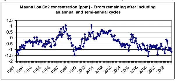
If we include the effects of a half-year cycle, we will reduce the residuals as evidenced in Fig. 3, where less structure can now be observed. The model for the concentration, then, becomes:

)) 2972 . 0 625 . 1992 ( sin( 8085 . 0 )) 5745 . 0 625 . 1992 ( 2 sin( 8854 . 2 ) 625 . 1992 ( 9247 . 1 77 . 354 ) ( 2 t t t t CO

The average of the residuals is 4.8e-6 ppm, and their standard deviation 0.4377 ppm. The work is not finished, however, as some structure remains, but the equation above might be a good

Figure 1. Comparison of original data and mathematical model approximation

Mauna Loa CO2 concentration - Original data and mathematical model

350 355 360 365 370 375 380 385 390 1993 1993 1994 1995 1996 1997 1998 1998 1999 2000 2001 2002 2003 2003 2004 2005 2006 2007 2008 2008

Original data points Mathematical Model

Figure 2. Residuals between original data and mathematical model approximation

Mauna Loa CO2 concentration [ppm] - Difference between original data and mathematical model after including an annual cycle

-3 -2 -1 0 1 2 3 1993 1993 1994 1995 1996 1997 1998 1998 1999 2000 2001 2002 2003 2003 2004 2005 2006 2007 2008 2008

Figure 3. Residuals after the annual and semi-annual cycles were also modeled

M auna Loa Co2 concentration [ppm] - Errors remaining after including an annual and semi-annual cycles

-2 -1.5 -1 -0.5 0 0.5 1 1.5 1993 1994 1994 1995 1996 1997 1998 1999 2000 2001 2002 2003 2004 2005 2005 2006 2007 2008

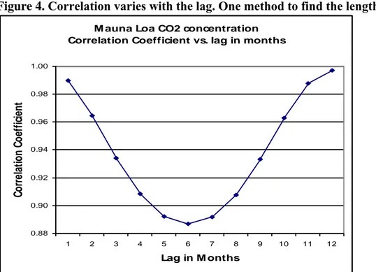
Instead of estimating the cycles by visual means, we could calculate the correlation of the CO2

stronger the linear relationship between the data points will be. If we do so, and calculate the correlation of two time series—one built with every data point corresponding to August of each year from 1963 to 2008, and another with the data points exactly one year before (from August 1962 to August 2007)—the correlation coefficient will be 0.9961, which strongly suggests the existence of an annual cycle. If, instead, we do the analysis every eleven months, the correlation will be smaller (0.9860) and even smaller if we increase the lag. As the series has an evident annual cycle, the correlation will exhibit a minimum at six months, and start increasing for a maximum at a lag of one year. This behavior is evident from Fig. 4. A more appropriate procedure to determine the cycles and their strength would have relied on Fourier analysis (spectral analysis), in the frequency domain.

Figure 4. Correlation varies with the lag. One method to find the length of a cycle…

M auna Loa CO2 concentration Correlation Coefficient vs. lag in months

0.88 0.90 0.92 0.94 0.96 0.98 1.00 1 2 3 4 5 6 7 8 9 10 11 12 Lag in M onths C o rr el at io n C o ef fi ci en t

When curve fitting is employed, the equation chosen for making the forecast or for projecting the historic data is generally the one that displays the highest correlation coefficient (usually using a "least-squares" criterion, which refers to any methodology which evaluates the relationship between a set of values and alternative estimators of those values by choosing that estimator for which the sum of the squared differences between the actual values and the estimated values is lowest) with the past data points. In certain cases, the practitioner may know beforehand that the system or parameter with which s/he is dealing cannot exceed 100 percent of the market. In such cases, only certain equations are selected a priori for use.

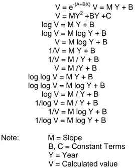
In the example above, two types of curves were used: a straight line, and a sinusoid. Many other curve types are available and may be used in fitting analyses; Figure 5 presents a set of curves typically used in curve fitting.

Figure 5. Common curve-fitting algorithms V = e-(A+BX) V = M Y + B V = MY2 +BY +C log V = M Y + B log V = M log Y + B V = M log Y + B 1/V = M Y + B 1/V = M / Y + B V = M /Y + B log log V = M Y + B log log V = M log Y + B

log V = M / Y + B 1/log V = M / Y + B 1/V = M log Y + B 1/log V = M log Y + B Note: M = Slope B, C = Constant Terms Y = Year V = Calculated value

Most curve-fitting software programs allow the user to designate a curve and selection of the proper general curve usually is based on minimum R2, a measure of the ―goodness of fit.‖ However, two different curve shapes can, for example, each fit the historical data well and yet produce markedly different extrapolations. In effect, selecting the curve shape may predetermine the forecast.

Averaging Methods

Data on historical trends can be smoothed using several methods. The arithmetic mean can be calculated and used as a forecast. However, this assumes that the time series is based on a fairly constant underlying process. Simple moving averages, which are computed by dropping the oldest observation and including the newest, provide a method of damping the influence of previous earlier data. Linear moving averages provide a more sophisticated averaging method better suited to addressing trends that involve volatile change. In effect, linear moving averages are a double moving average, that is, a moving average of a moving average.

Exponential smoothing refers to a class of methods in which the value of a time series at some point in time is determined by past values of the time series. The importance of the past values declines exponentially as they age. This method is similar to moving averages except that, with exponential smoothing, past values have different weights and all past values contribute in some way to the forecast.

Exponential smoothing methods are useful in short-term forecasting. They can often produce good forecasts for one or two periods into the future. The advantage of exponential smoothing is in its relatively simple application for quickly producing forecasts of a large number of variables. For this reason, this method has found wide application in inventory forecasting. Exponential smoothing should not be used for medium-or long-term forecasts or for forecasts in which

change may be rapid. Such forecasts depend heavily on the most recent data points and thus tend to perform well in the very short term and very poorly in the long term.

Regression analysis

The technique of regression analysis allows building a function of a dependent variable (the response variable or output) in terms of independent variables (the explanatory variables or inputs). This function can later be used for inference, forecasting, hypothesis testing, or determining causality. In general, the form of the equation that relates the dependent to the independent variables is:

where y(t) is the estimate of a real response variable y (t), and c0, c1, …, cn are the constants

(sometimes called coefficients). The variables x1 to xn are the explanatory (linearly independent)

variables, and the error term u(t) represents a random variable in which we concentrate all the unknowns that exist between our ideal model and the real system in question. As all the terms are evaluated at a time t, the output will also be determined at time t, but this single evaluation or measurement is not sufficient to determine all the (n+1) constants. In general, we will have m measurements or data points:

Note that we can include further functionality in the equations by introducing new variables such as cross-products (x1 * xn) or other functions (ln(x1), cos(x1)). Also, an added advantage of the

method is that once we calculate the constants, each of the coefficients (say, c1) represents the

gradient of the estimate of y(t) with respect to the variable or set of variables that it is multiplying (say, x1), maintaining the rest of the variables constant.

Assuming that the variables are not linearly related, we need (n+1) measurements to have a unique solution for the constants, or more than (n+1) measurements to have an over-determined system with an infinite number of solutions. As we are interested in only one solution, we impose the additional criterion of minimizing the sum of the residuals squared

2 1 2 )) ( ) ( ( ) ( min _{i i} m t y t y t e

The usual method of determining the constants is by least squares, details of which are beyond the scope of the present chapter, but that most statistics software packages can solve. In the case of a two-constant (c0 and c1) system the solutions are

) ( ) ( ) ( ) ( ) (t c₀ c₁x₁ t c₂x₂ t c x t u t y  _{n n} ) ( ) ( ) ( ) ( ) ( ) ( ) ( ) ( ) ( ) ( ) ( ) ( 2 2 1 1 0 2 2 2 2 2 1 1 0 2 1 1 2 2 1 1 1 0 1 m n n m m m n n n n t x c t x c t x c c t y t x c t x c t x c c t y t x c t x c t x c c t y    

Forecasting with multiple-regression analysis requires:

Sets of historical values for each of the independent variables, and the dependent variable for the same time period.

Independently derived — extrapolated or forecasted — values of the

independent variables for each time or occasion when a value of the dependent variable is to be computed.

Many high-quality software statistical packages facilitate the regression process. Not only do they produce high-quality graphs of actual and calculated data, but also they produce a wealth of information regarding how well the regression matches actual data.

To illustrate the use of the technique, if our interest is to analyze how the Gross National Product (GNP) of the USA behaved between 1959 to the present, we can try to model it as a function of the monetary base M225. The expression that links the input (M2) to the single output (GNP) is known to have the form

)) ( 2 ln( )) ( ln(GNP t c₀ c₁ M t

where t is January of any year between 1959 and 2008, and c0 and c1 are constants that have to

be determined. Other functional expressions can be used, but this will suffice for our purposes. In many applications, it is not advisable to use all the data to determine the constants. Usually, a large portion of the data allows determining c0 and c1, and the rest is used to check how the

function estimates the remaining years. Otherwise, in some cases, an effect of overestimation might occur, where the estimated constants fit the data ―too well‖ in the estimation interval, but poorly outside. In our case, we will rely on the data set from 1959 to 1999 to estimate the constants, and will use the M2 data from 2000 to 2008 to check how the GNP is predicted. Using the equations above or a software package, we can find that

)) ( 2 ln( 05888 . 1 1623 . 0 )) ( ln(GNP t M t

with a R2 coefficient of 0.997 and the t-stats indicated below the corresponding parameters. We can also express the above equation as

05888 . 1 ) ( 2 1.1762 ) (t M t GNP

and a graphical representation of the original data and the regressed estimate can be found in Figure 6.

25

M2 includes all physical currency, accounts of the central bank that can be exchanged for physical currency— minus reserves—plus checking, savings, and money market accounts, and small certificates of deposit. In the example, GNP data was retrieved from the Federal Reserve Bank of St. Louis, at http://research.stlouisfed.org/fred2/ Monetary base data from the Federal Reserve at http://www.federalreserve.gov/releases/h6/hist/h6hist1.txt.

2 1 ) ( ) )( ( x x y y x x c i i i x c y c0 1

Figure 6: Estimation of the USA GNP as a function of the monetary base ln(GNP(t)) = a + b*ln(M2(t)) [billions USD] -2,000 4,000 6,000 8,000 10,000 12,000 14,000 16,000 1959 1962 1965 1968 1971 1974 1977 1980 1983 1986 1989 1992 1995 1998 2001 2004 2007 Actual GNP Estimated GNP

One problem in regression analysis is to find appropriate independent variables that promise a relationship with the dependent variable. This can be approached using multivariate correlations, by identifying the correlation coefficients that exist between potential variables. Figure 7

illustrates a typical correlation coefficient printout. The data were drawn from the World Bank‘s database and are for the United States over the years from 1985 to 2005. The variables are:

Year

Electricity production from nuclear sources (% of total) Adjusted savings: carbon dioxide damage (% of GNI) Unemployment (% labor force)

GDP per unit of energy use (constant 2005 PPP $ per kg of oil equivalent) Population growth (annual %)

Research and development expenditure (% of GDP) Fossil fuel energy consumption (% of total)

GDP per capita, PPP (constant 2005 international $) Life expectancy at birth, total (years)

Using a commercially available statistical package, the coefficients are shown in Figure 7: Figure 7 Multivariate Correlations

Nuclear Electricity Production CO2 Damage % GNP Unemploy-ment % GDP per unit of energy use Population Growth % Fossil Energy Consumption GDP/Cap Nuclear Electricity Production 1.0000 -0.6078 -0.3712 0.5521 0.4986 -0.8589 0.5962 CO2 Damage % GNP -0.6078 1.0000 0.6045 -0.9799 -0.0691 0.5211 -0.9808 Unemployment % -0.3712 0.6045 1.0000 -0.5593 0.0747 0.2600 -0.6452 GDP per unit of energy use 0.5521 -0.9799 -0.5593 1.0000 0.0051 -0.4590 0.9893 Population Growth % 0.4986 -0.0691 0.0747 0.0051 1.0000 -0.7638 0.0324 Fossil Energy Consumption -0.8589 0.5211 0.2600 -0.4590 -0.7638 1.0000 -0.4979 GDP/Cap 0.5962 -0.9808 -0.6452 0.9893 0.0324 -0.4979 1.0000

These data tell us, for example, that there is a relatively high negative correlation between fossil fuel energy consumption and nuclear electricity production (-0.8589) and, similarly a very high negative correlation exists between GDP per unit of energy use and CO2 damage. These results

would lead us to expect that a good regression equation for GDP per unit of energy consumption would have as independent variables CO2 Damage as a % of GNP, and GDP/capita.

Dynamic Systems Modeling

This CD ROM contains a chapter on ―The Systems Perspective: Methods and Models for the Future‖ which provides detailed descriptions of system models. The next few paragraphs deal with a portion of the same material because dynamic systems modeling, in many instances, offers an alternative technique to statistical models.

In dynamic systems modeling, an attempt is made to duplicate the system being modeled in the form of equations, not solely by drawing on statistical relationships among variables, but rather by logic and inference about how the system works. For example, using regression to forecast the number of people who live in Accra, Ghana, one might find a very precise, but spurious, correlation with the number of apples sold in New York. The statistics might appear excellent, but the logic flawed. Furthermore, the coefficients produced in a regression analysis have no actual physical meaning. The perspective changes in dynamic systems modeling. This method starts with an idea about how the system functions and gives meaning to the coefficients. For example, suppose we want to construct a model for use in forecasting the population of Accra, Ghana. A time-series analysis might use historical population data, fit a curve, and by using the equation, extend the data into the future. A regression analysis would relate population to factors considered important, such as life expectancy, education, immigration, unemployment, etc. In either case the equations would relate the dependent variable, population, to the

independent variables such as time, life expectancy, education, etc.. The coefficients of the equations would be numbers that have no physical meaning. On the other hand, in dynamic modeling, the objective would be the same, but the modeling process would start with the definition of a system that would logically include population as an output. In the equations, the coefficients would have some meaning. For example:

Population in year2= Population in year1 + Births in year1 – Deaths in year 1 + net migration in year1

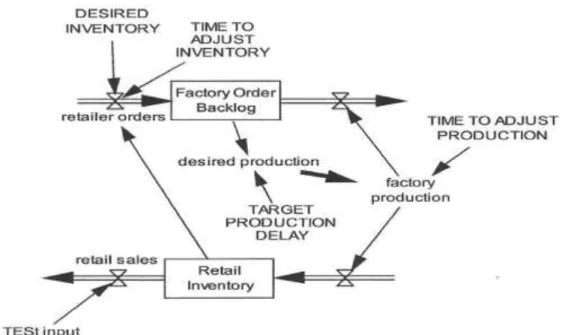
Dynamic systems modeling is complicated but has the advantage of forcing attention on how things really work. Systems dynamics models of the sort first developed by J. Forrester (1961) were used in the construction of the World Dynamics model for the Limits to Growth (Meadows, 1973) study; these models involve feedback loops, stocks and flows. These three seemingly simple elements can be assembled into systems that exhibit complex and unexpected behavior. For example the model shown in Figure 8 depicts a production/ordering/retailing system (Kirkwood, 2001)

Figure 8. A production/ ordering/ retailing system (Kirkwood, 2001)

The ―valves‖ labeled ―retailer orders,‖ ―retail sales,‖ and ―factory production‖ control flows; the boxes labeled ―Factory Order Backlog‖ and ―Retail Inventory‖ represent stocks and the lines with arrows represent flows. Kirkwood (2001) gives an excellent set of instructions on how to build such models. As noted, the chapter on ―The Systems Perspective: Methods and Models for the Future‖ contains much more detail about such models and provides references to software for forming systems models and their equations.

If we were to use only time and the initial conditions of the explanatory variables we would be able to create only one time trajectory of the dependent variable. However, we know that in real time applications the parameters in the equations can vary and that the model will be subject to disturbances. Conscious of these variations, we will then have to perform many simulations, changing the parameters, the initial conditions, and the disturbances, each combination creating a different scenario. This qualitative description is not far from the spirit of the Monte Carlo method26, an automated procedure born immediately after the end of World War II that mixed the concepts of statistical sampling with the computer‘s versatility and speed.

26

Named by Nicholas Metropolis (1915-1999), after an idea of Stanislaw Ulam (1909-1984), with intervention of John von Neumann (1903-1957). See Metropolis, Nicholas (1987). ―The Beginning of the Monte Carlo Method,‖ Los Alamos Science, Special Issue, pp. 125-130. The article notes that Enrico Fermi (1901-1954) had

Validation

Whether the models are statistically derived or are of the systems variety, the analyst usually must also perform a validation step. Validation usually is accomplished by one or more of the following methods:

Computing the cumulative absolute error between the true historical data and the values produced by the statistical or simulation model. Usually this is in the form of the

statistical measure, r2 (more on this in the next section of this chapter).

Demonstrating the ability of the model to reproduce recent data by constructing the models using data that does not include the most recent period, running the model to ―forecast‖ that period, and then comparing the actual data from that period to the model‘s results.

Observing the dynamic behavior of the model and comparing it to real life. If the real system produces periodic peaks, for example, the model should be expected to do so as well.

Performing sensitivity tests. The input data can be varied slightly to observe the model‘s

response which should resemble the expected response of the real system. Excessive sensitivity may indicate that the system can be chaotic and that the feedback can lead to instability.

Testing the Residuals

Various tests have been developed to perform a conscientious analysis of the residuals. Among other points on which to focus our attention, the main two are (a) verifying that the variance does not change in time and (b) the residuals behave with a distribution close to normal.

(a) Constant variance (homoscedasticity): Besides relying on a visual plot of the variance of the residuals, the whole set of residuals could be divided into two parts (one set for the first half of the time series and another set for the rest) and an F-Test Two-Sample could be made on the sets to determine if the hypothesis that the population variances are the same could be accepted. If the variance changes in time, weighted least squares (WLS) could be used instead of ordinary least squares (OLS).

(b) Normality: The assumption that the residuals are normally distributed impacts the calculation of other statistical indicators27. To test normality, besides visually checking a histogram of the residuals or calculating the first four moments, various tests can be used (Anderson-Darling, D‘Agostino‘s K-squared, Lilliefors, Pearson‘s chi-square, Shapiro-Wilk), the Cramer-von-Mises criterion, or the QQ (quantile-quantile) plots.

27

To determine quantitatively how good the estimates of the parameters are, firstly, we can calculate the coefficient of determination, R2, which indicates the proportion of the dependent variable that can be attributed to all the independent variables acting together. It can also be interpreted as the explained variance, the ratio between the variance as predicted by the model with the total variance of the data. R2 can vary between 0 and 1, is not affected by changes in the measurement units, and a modification of it (adjusted R2) considers the effect of small samples. This will indicate how adequate all of the parameters are in fitting the data. Secondly, we can quote the t-statistic of each of the parameters, sometimes displayed in brackets below each of the parameters. The t-statistic (t-stats, t-ratio, t-value) indicates how far the estimated coefficient is from being a specified fixed value (0 or other numerical value) given the amount of data used: the further it is, the more statistically significant it becomes. From the t-stats tables, for example, for a t-stats of 2, only 5 samples would be necessary to have a statistical significance of 90%, but more than 60 samples to have a statistical significance of 95%. For more statistical significance, more data are required.

How good are the estimates of the constants? The well-known Gauss-Markov theorem states that the best linear unbiased estimator of the coefficients is the least squares estimator if the model is linear and the errors u(t) have a zero mean, are uncorrelated, and have a constant variance (thus, it is not necessary for the errors to be normally distributed). For this reason we try to remove all possible recognizable behavior from the noise term and attribute it in some functional form to the equations expressing y(t). Once the errors do not have a recognizable structure, the estimated constants are the best linear unbiased estimates obtainable.

In addition to these requirements on the errors (residuals), the independent variables should be linearly independent.

Specific regression methods can be invoked in special circumstances. For example, if the dependent variable y(t) is a probability, bounded by definition between 0 and 1, a logistic

regression can be performed. The function estimate is defined as logit28 and will be regressed as

usual. For example, for a linear regression:

n nx c t x c t x c c p p p Logit ) ( ) ( )  1 log( ) ( _{0 1 1 2 2} or, equivalently, ) ( 1 1 ) ( ) ( _{z t} e t p t y ; z(t) c0 c1x1(t) c2x2(t)  cnxn(t)

Examples to predict political and economic country risks based on logit regressions have been developed, where the probability of a certain risk (i.e., unrest, default) is modeled as a function

28

of regressors (literacy, military budget as a percentage of total budget, public debt, GNP, etc.).29 The independent variables can also be categorical (that is, binaries, indicating data points which might exist or not). The model can also be extended to situations that have a plateau with decreasing growth rates (i.e., population models30). The next one is one such example,

t c o e c c t y 2 1 ^ 1 ) (

If, instead of a probability, the dependent variable y(t) can be expressed as a specific function of a probability known as probit31 (probability unit), then the regression can be performed on the probit of the observed probability.

) ( ) ( ) ( ) ( ) (p 1 p c₀ c₁x₁ t c₂x₂ t c x t probit  _{n n}

where Φ is the standard cumulative normal probability distribution.

Probit regressions, also used for categorical independent variables, are less common than logit regressions because the coefficients are less easily interpreted than logits, which are simply odds ratios.

One of the most versatile methods is the stepwise regression, in which all combinations of variables are tested until the best one is found32. Instead of simply combining variables we might want to combine processes (autoregressive, differencing, moving average). In this case, the most powerful methods are ARIMA33 (AutoRegressive, Integrated, Moving Average) and GARCH34 (Generalized AutoRegressive Conditional Heteroskedasticity, an autoregressive-moving average model with varying variance), for which specialized literature should be consulted.

29

McGowan, Jr., Carl et al (2005). ―Using Multinomial Logistic Regression of Political and Economic Risk Variables for Country Risk Analysis of Foreign Direct Investment Decisions,‖ Southwestern Economic Proceedings, Vol. 32. Proceedings of the 2004 Conference, Orlando, Florida.

30

Keyfitz, Nathan et al. (1968). ―World Population: An Analysis of Vital Data,‖ Chicago, University of Chicago Press, p. 215

31

Introduced by Chester Ittner Bliss in 1934. 32

Efroymson, M. (1960). ―Multiple Regression Analysis,‖ in Ralston, A. and Wilf, H. (Eds.) ―Mathematical Methods for Digital Computers,‖ Wiley.

33

Box, George and Jenkins, Gwilym (1970). ―Time Series Analysis: Forecasting and Control,‖ San Francisco, Holden Day. ARIMA models are used by the U.S. Census Bureau.

34

Bollerslev, Tim (1986). ―Generalized Autoregressive Conditional Heteroskedasticity,‖ Journal of Econometrics, Vol. 31, pp. 307-327.

III.

S

W

M

Although time-series analysis is quick and easy, it provides little fundamental understanding of the forces that will shape future behavior. The same criticism can be raised for almost all forms of statistically based models- from regression to econometrics. Since the future is predicated solely on the past without an underlying feel for causal factors, time series is a naive but often useful forecasting method.

While various forms of explanatory or causal forecasting strive to explain fundamental causal relationships, those too are predicated on past behavior and therefore also may present a naive forecast. The analyst must ask if the relationships intrinsic to the system being modeled will hold in the future.

Major Strengths of Regression

The strength of regression as a forecasting method is that it capitalizes on historical relations between the predicted (dependent) and predictor (independent) variables. It uses all the

information in the historical data pairs to determine the future values of the predicted variables. The "goodness of fit" of the Yc to the historical Y values can be used to compute a measure of

the strength of the linear relationship between the historical X, Y pairs which then can be used to calculate "confidence limits" or probable upper and lower bounds for the predicted values of Y. In general, the closer the Yc to the historical Y values, the narrower the confidence limits; that is,

the actual values of Y are less likely to depart from the predicted values.

The correlation coefficient is an index that can be used to calculate a figure of merit from the accuracy with which the calculated values of Y, Yc match the actual past-history data. The

square of the correlation coefficient ranges from 0 through 1. A value of 0 means total failure of the Yc values to correspond with the corresponding Y values. A value of 1 for the square of the

correlation coefficient means that the Y and Yc values correspond exactly. Values between 0

and 1 may be interpreted as expressing the proportion of variability in the historical Y values that could be accounted for by the calculated linear relationship between X and Y.

Major Limitations of Regression

The method of least squares, as commonly used, implies that the predicted values of the independent variable (X) are devoid of error or uncertainty; that is, the only possible error or uncertainty is in values of the dependent variable (Y). Often this assumption is questionable. For example, independent variables can be forecast incorrectly. Take a specific example: suppose we want to forecast the prime interest rate and develop a good statistical equation relating the

Consumer Price Index (CPI) and the prime interest rate. A forecast of the future CPI trend may then be used to generate a forecast of the prime interest rate, using bi-variate linear regression. Accuracy of this forecast depends on how strongly the past CPI values and prime interest rate are related and on how accurately the future CPI trend is predicted. The latter source of inaccuracy

is not normally taken into account in calculating upper and lower bounds for the forecasted values of the dependent variable or, more generally, in evaluating the accuracy of this forecasting method.

When the past-history data are subject to error, the effect of the error makes the predicted values of Y vary less than they should. Values of Y that should fall below the mean will generally be forecast as such, but less so than they should be, similarly for values that should be above the mean. The greater the "noise" in the past history, the greater this effect; and no way exists using this method to distinguish a weak relationship between X and Y from a strong relationship that is obscured by noise or errors of measurement.

The methods, as commonly applied, assume that all past-history data pairs are equally important. While "weighted" data pairs can be used to generalize, the method is not common.

The method fundamentally generates a "regression forecast." The forecast of Y depends on a prior forecast of X. Similarly, the forecast of X might depend upon a prior forecast of W. But somewhere in this series a forecast must exist that does not depend on another forecast. One way to break the chain is to have time itself as the predictor or independent variable. This option, however, necessarily results in the predicted (dependent) variable, which depends only on time, either increasing or decreasing without limit over time.

One might assume that these difficulties and pitfalls lead to the conclusion that dynamic models, featuring cause and effect relationships are the answer. But there are weaknesses here too. The underlying assumption is that it is possible to conceptually bound and describe a functioning system, that is, to distinguish between endogenous and exogenous aspects. This is often difficult. Further, these methods assume that the structure depicted in causal loop diagrams are invariant with time and this assumption can be wrong when momentous changes affect not only the stocks, flows, and feedback but the structure of the model itself.

IV.

F

M

Statistical methods described here rely heavily on the assumption that forces shaping history will continue to do so. The frontiers of statistical methods must surely include techniques to test that assumption and, where found wanting, permit the introduction of perceptions about change. Trend Impact Analysis, Probabilistic System Dynamics, Cross Impact Analysis, Interax: all of these methods attempt to meld judgment with statistics.

Staying strictly within the bounds of statistics, some research directions that could benefit the field include:

Developing methods that test time series for chaos (see section Frontiers of Futures Research). Unless special cases are involved, fitting chaotic time series using any of the techniques suggested here will probably be unproductive.

example, using an S-shaped function when regressing variables that relate to technological maturation or substitution.

Simulating policies in regression models. To date, "dummy variables" whose value is either zero or one have been used in regression studies to indicate the presence or absence of a policy. This method is not refined.

Using improved clustering or multidimensional scaling techniques to improve the efficiency of searching for variables that can fit in a group or relate to one another. Including nonlinear relations in simulation models, which can sometimes result in

apparent chaotic behavior.

V.

W

I

D

I

Fortunately statistical analysis is facilitated by a large number of software programs that are growing in sophistication. These programs have made more sophisticated quantitative analysis widely available and relatively inexpensive to forecasters and planners. The most sophisticated methods tend to be used by consultants, mathematicians, and econometricians who have devoted considerable time to the study of the subject.

There are many fine packages to perform SM and related activities. Currently, 56 packages are listed in a comparison of statistical packages35, of which ADamSoft, BrightStat, Dataplot, gretl, MacAnova, OpenEpi, PSPP, R, R Commander, RKWard, SalStat, and SOCR are free.

Many packages have a large user base: Gauss, Mathematica, Minitab, R, S, SAS, SPlus, SPSS. Software packages are available from numerous sources, including:

SYSTAT Inc.

1800 Sherman Avenue Evanston, IL 60201

(708) 864-5670, Fax (708) 492-3567;

http://www.cranessoftware.com/products/products/systat.html Smart Software, Inc.

(Charles Smart, President) 4 Hill Road

Belmont, MA 02178

(617) 489-2743 Fax (617) 489-2748; http://www.smartcorp.com/ SPSS, Inc.

444 North Michigan Ave., Suite 3000 Chicago, IL 60611

(312) 329-2400, Fax (312) 329-3668; http://www.spss.com/

35

SAS Institute Inc. SAS Campus Drive Cary, NC 27513 (919)677-8000, Fax (919)677-8123; http://www.sas.com/ TSP International P.O. Box 61015 Palo Alto, CA 94306 (415) 326-1927; http://www.tspintl.com/ The MathWorks, Inc.

3 Apple Hill Drive Natick, MA 01760-2098 UNITED STATES Tax ID# 942960235 Phone: 508-647-7000 Fax: 508-647-7001; http://www.mathworks.com/products/econometrics/?s_cid=HP_FP_ML_EconometricsToolbox Applications of statistical methods span a vast canvas and range from analysis of astronomical bodies to genetics, from analysis of breaks in water systems to disease epidemics. Wherever there are data, there are statistical studies. Some of these are summarized below to illustrate the broad scope of applications.

Boyacioglu et al (2009) applied statistical methods to the prediction of bank failures in Turkey. Their approach include several methods, in particular ―multivariate statistical methods; multivariate discriminant analysis, k-means cluster analysis and logistic regression analysis.‖

Zhang (2009) in his paper, ―Likelihood-Based Confidence Sets For Partially Identified Parameters,‖ applies statistical techniques of the sort described here to complete data sets with missing data, including data that has been deleted as a result of censorship.

Bordley, R., and Bier (2009) address the problem of updating beliefs about the

relationships among variables included in a regression model or a simulation model. The paradox is that the original models may be based on beliefs which are revised as a result of the model. How then can the models be updated?

Ye et al. (2009) describe a new statistical technique which has proven useful in the analysis of near-infrared spectroscopy (NIRS) in the measurement of brain activity. They have developed ―a. a new public domain statistical toolbox known as NIRS-SPM.‖ In their approach‖NIRS data are statistically analyzed based on the general linear model (GLM) …The p-values are calculated as the excursion probability of an inhomogeneous random field… dependent on the structure of the error covariance matrix and the interpolating kernels. NIRS-SPM not only enables the calculation of activation maps of oxy-, deoxy-hemoglobin and total hemoglobin, but also allows for the super-resolution localization, which is not possible using conventional analysis tools.‖

We have only scratched the surface of SM and, overall, we have simplified the issues to the extreme, so much so that it would seem that just with a handbook on statistics under the arm, it would be possible to attack any modeling problem. On the contrary, if we have learned anything during the previous century is that we have not stopped marveling at the complexity of the systems that we wish to simulate or control, and that the most ―impressive theories have provided us … not so much [with] a solution of the problem[s] as [with] a demonstration of [their] deep intractability.‖ 36

At their core, SM techniques rely on using a model as a substitute for reality, and we should be conscious that the model will always be an inaccurate representation of a phenomenon that happens in real life. The question is how far we may allow our model to deviate from reality, and, to help our decision to be evaluated quantitatively, we need to use formal numerical procedures.

In that sense, the inputs, the model, and the outputs need to be carefully treated by the modeler. The inputs (including uncertainties) have to represent those found in reality. The model

(including changes of parameters) has to contain all the modes of behavior that are relevant for the study in question (i.e., neither too detailed nor too general). Further, for the same type of inputs, the outputs have to track real-life measurements within a specified tolerance. Specific techniques exist to test these considerations, and the literature cited in the preceding pages and in the bibliography should be consulted for more details.

36

In particular, it can be said that most of the scientific efforts for the last 50 or 100 years have been directed to model situations far from equilibrium and the steady state. For a glimpse at general issues related to modeling, including the philosophy of modeling, complex systems, chaos, nonlinearities, and comments about the Club of Rome models as more prescriptive than predictive, see Simon (1990), op. cit. in Note 16.

BIBLIOGRAPHY

Armstrong, J. Scott (ed.), ―Principles of Forecasting: A Handbook for Researchers and Practitioners,‖ Springer, 2001

Arthurs, A.M. (1965). Library of Mathematics: Probability Theory. Routledge.

Ayres, Robert U. "Envelope Curve Forecasting." Technological Forecasting for Industry and

Government. Edited by James R. Bright. New Jersey: Prentice-Hall, Inc., 1968, pp. 77-94.

Ayres, Robert U. "Extrapolation of Trends." Technological Forecasting and Long-Range

Planning. New York: McGraw-Hill, 1969, pp. 94-117.

Benton, William K. "Time Series Forecasting." Forecasting for Management. Massachusetts: Addison-Wesley, 1972, pp. 67-139.

Bordley, R., and Bier, V., ―Updating Beliefs About Variables Given New Information On How Those Variables Relate,‖ European Journal of Operational Research, Volume 193, Issue 1, 16 February 2009, pp. 184-194

Boyacioglu, M.A., Kara, Y. Baykan, O.K., ―Predicting Bank Financial Failures Using Neural Networks, Support Vector Machines And Multivariate Statistical Methods: A Comparative Analysis In The Sample Of Savings Deposit Insurance Fund (SDIF) Transferred Banks In Turkey,‖ Expert Systems with Applications ,Volume 36, Issue 2 PART 2, March 2009, pp. 3355-3366

Bright, James R. "Trend Extrapolation." A Brief Introduction to Technology Forecasting:

Concepts and Exercises. Austin, Texas: Pemaquid Press, 1972, pp. 6-1 to 6-70.

Burington, R.S. et al (1970). Handbook of Probability and Statistics with Tables. McGraw-Hill. Burnham, K. P. and Anderson, D. R. (2002) Model Selection and Multi-Model Inference: A

Practical Information Theoretic Approach. New York: Springer, second edn.

Claeskens, G. and Hjort, N. L. (2008) Model Selection and Model Averaging. Cambridge: Cambridge University Press.

Congressional Research Service. "Trend Extrapolation." Long-Range Planning. Prepared for the Subcommittee on the Environment and the Atmosphere. Washington, D.C.: U.S.

Government Printing Office, May 1976, pp. 434-443.

Conover, W.J. (1980). Practical Nonparametric Statistics (2nd ed.). Wiley, N.Y. Davison, A. C. (2003) Statistical Models. Cambridge: Cambridge University Press.