2014 JINST 9 P06009
PUBLISHED BYIOP PUBLISHING FORSISSAMEDIALABRECEIVED: March 10, 2014 ACCEPTED: April 23, 2014 PUBLISHED: June 6, 2014
Alignment of the CMS tracker with LHC and cosmic
ray data
The CMS collaboration
E-mail:[email protected]
ABSTRACT: The central component of the CMS detector is the largest silicon tracker ever built.
The precise alignment of this complex device is a formidable challenge, and only achievable with a significant extension of the technologies routinely used for tracking detectors in the past. This article describes the full-scale alignment procedure as it is used during LHC operations. Among the specific features of the method are the simultaneous determination of up to 200 000 alignment parameters with tracks, the measurement of individual sensor curvature parameters, the control of systematic misalignment effects, and the implementation of the whole procedure in a multi-processor environment for high execution speed. Overall, the achieved statistical accuracy on the
module alignment is found to be significantly better than 10µm.
KEYWORDS: Particle tracking detectors; Detector alignment and calibration methods (lasers,
sources, particle-beams); Large detector systems for particle and astroparticle physics
2014 JINST 9 P06009
Contents
1 Introduction 1
2 Tracker layout and coordinate system 3
3 Global position and orientation of the tracker 5
4 Methodology of track based internal alignment 8
4.1 Track parameterisation 8
4.2 Alignment parameterisation 10
4.3 Hierarchical and differential alignment by using equality constraints 11
4.4 Weak modes 12
4.5 Computing optimisation 14
5 Strategy of the internal alignment of the CMS tracker 15
6 Monitoring of the large structures 18
6.1 Monitoring of the strip tracker geometry 18
6.2 Monitoring of the pixel detector geometry with tracks 19
7 Statistical accuracy of the alignment 20
8 Sensor and module shape parameters 24
9 Control of systematic misalignment 29
9.1 Monitoring of the tracker geometry with Z ! µµ events 29
9.2 Monitoring of the tracker geometry with the CMS calorimeter 30
9.3 Sensitivity to systematic misalignment 32
10 Summary 33
The CMS collaboration 39
1 Introduction
The scientific programme of the Compact Muon Solenoid (CMS) experiment [1] at the Large
Hadron Collider (LHC) [2] covers a very broad spectrum of physics and focuses on the search
for new phenomena in the TeV range. Excellent tracking performance is crucial for reaching these goals, which requires high precision of the calibration and alignment of the tracking devices. The
task of the CMS tracker [3, 4] is to measure the trajectories of charged particles (tracks) with
2014 JINST 9 P06009
efficiency [5]. According to design specifications, the tracking should reach a resolution on the
transverse momentum, pT, of 1.5% (10%) for 100GeV/c (1000GeV/c) momentum muons [5]. This
is made possible by the precise single-hit resolution of the silicon detectors of the tracker and the high-intensity magnetic field provided by the CMS solenoid.
The complete set of parameters describing the geometrical properties of the modules com-posing the tracker is called the tracker geometry and is one of the most important inputs used in the reconstruction of tracks. Misalignment of the tracker geometry is a potentially limiting factor for its performance. The large number of individual tracker modules and their arrangement over a large volume with some sensors as far as ⇡6 m apart takes the alignment challenge to a new stage compared to earlier experiments. Because of the limited accessibility of the tracker inside CMS and the high level of precision required, the alignment technique is based on the tracks reconstructed by the tracker in situ. The statistical accuracy of the alignment should remain significantly below
the typical intrinsic silicon hit resolution of between 10 and 30µm [6, 7]. Another important
as-pect is the efficient control of systematic biases in the alignment of the tracking modules, which might degrade the physics performance of the experiment. Systematic distortions of the tracker geometry could potentially be introduced by biases in the hit and track reconstruction, by inaccu-rate treatment of material effects or imprecise estimation of the magnetic field, or by the lack of sensitivity of the alignment procedure itself to such degrees of freedom. Large samples of events with different track topologies are needed to identify and suppress such distortions, representing a particularly challenging aspect of the alignment effort.
The control of both the statistical and systematic uncertainties on the tracker geometry is cru-cial for reaching the design physics performance of CMS. As an example, the b-tagging
perfor-mance can significantly deteriorate in the presence of large misalignments [5, 8]. Electroweak
precision measurements are also sensitive to systematic misalignments. Likewise, the imperfect knowledge of the tracker geometry is one of the dominant sources of systematic uncertainty in the measurement of the weak mixing angle, sin2(qeff) [9].
The methodology of the tracker alignment in CMS builds on past experience, which was in-strumental for the fast start-up of the tracking at the beginning of LHC operations. Following
simu-lation studies [10], the alignment at the tracker integration facility [11] demonstrated the readiness
of the alignment framework prior to the installation of the tracker in CMS by aligning a setup with approximately 15% of the silicon modules by using cosmic ray tracks. Before the first proton-proton collisions at the LHC, cosmic ray muons were recorded by CMS in a dedicated run known
as “cosmic run at four Tesla” (CRAFT) [12] with the magnetic field at the nominal value. The
CRAFT data were used to align and calibrate the various subdetectors. The complete alignment of the tracker with the CRAFT data involved 3.2 million cosmic ray tracks passing stringent quality requirements, as well as optical survey measurements carried out before the final installation of
the tracker [13]. The achieved statistical accuracy on the position of the modules with respect to
the cosmic ray tracks was 3–4µm and 3–14 µm in the central and forward regions, respectively.
The performance of the tracking at CMS has been studied during the first period of proton-proton
collisions at the LHC and proven to be very good already at the start of the operations [14–16].
While the alignment obtained from CRAFT was essential for the early physics programme of CMS, its quality was still statistically limited by the available number of cosmic ray tracks, mainly in the forward region of the pixel detector, and systematically limited by the lack of kinematic
2014 JINST 9 P06009
diversity in the track sample. In order to achieve the ultimate accuracy, the large track sample accumulated in the proton-proton physics run must be included. This article describes the full alignment procedure for the modules of the CMS tracker as applied during the commissioning campaign of 2011, and its validation. The procedure uses tracks from cosmic ray muons and proton-proton collisions recorded in 2011. The final positions and shapes of the tracker modules have been used for the reprocessing of the 2011 data and the start of the 2012 data taking. A similar procedure has later been applied to the 2012 data.
The structure of the paper is the following: in section 2 the tracker layout and coordinate
system are introduced. Section3describes the alignment of the tracker with respect to the magnetic
field of CMS. In section4the algorithm used for the internal alignment is detailed with emphasis
on the topic of systematic distortions of the tracker geometry and the possible ways for controlling them. The strategy pursued for the alignment with tracks together with the datasets and selections
used are presented in section 5. Section 6 discusses the stability of the tracker geometry as a
function of time. Section 7presents the evaluation of the performance of the aligned tracker in
terms of statistical accuracy. The measurement of the parameters describing the non-planarity of
the sensors is presented in section8. Section 9describes the techniques adopted for controlling
the presence of systematic distortions of the tracker geometry and the sensitivity of the alignment strategy to systematic effects.
2 Tracker layout and coordinate system
The CMS experiment uses a right-handed coordinate system, with the origin at the nominal colli-sion point, the x-axis pointing to the centre of the LHC ring, the y-axis pointing up (perpendicular to the LHC plane), and the z-axis along the anticlockwise beam direction. The polar angle (q) is measured from the positive z-axis and the azimuthal angle (j) is measured from the positive x-axis in the x-y plane. The radius (r) denotes the distance from the z-axis and the pseudorapidity (h) is
defined ash = ln[tan(q/2)].
A detailed description of the CMS detector can be found in [1]. The central feature of the
CMS apparatus is a 3.8 T superconducting solenoid of 6 m internal diameter.
Starting from the smallest radius, the silicon tracker, the crystal electromagnetic calorimeter (ECAL), and the brass/scintillator hadron calorimeter (HCAL) are located within the inner field volume. The muon system is installed outside the solenoid and is embedded in the steel return yoke of the magnet.
The CMS tracker is composed of 1440 silicon pixel and 15 148 silicon microstrip modules
organised in six sub-assemblies, as shown in figure 1. Pixel modules of the CMS tracker are
grouped into the barrel pixel (BPIX) and the forward pixel (FPIX) in the endcap regions. Strip modules in the central pseudorapidity region are divided into the tracker inner barrel (TIB) and the tracker outer barrel (TOB) at smaller and larger radii respectively. Similarly, strip modules in the endcap regions are arranged in the tracker inner disks (TID) and tracker endcaps (TEC) at smaller and larger values of z-coordinate, respectively.
The BPIX system is divided into two semi-cylindrical half-shells along the y-z plane. The TIB and TOB are both divided into two half-barrels at positive and negative z values, respectively. The pixel modules composing the BPIX half-shells are mechanically assembled in three concentric
2014 JINST 9 P06009
Figure 1. Schematic view of one quarter of the silicon tracker in the r-z plane. The positions of the pixelmodules are indicated within the hatched area. At larger radii within the lightly shaded areas, solid rectangles represent single strip modules, while hollow rectangles indicate pairs of strip modules mounted back-to-back with a relative stereo angle. The figure also illustrates the paths of the laser rays (R), the alignment tubes (A) and the beam splitters (B) of the laser alignment system.
layers, with radial positions at 4cm, 7cm, and 11cm in the design layout. Similarly, four and six layers of microstrip modules compose the TIB and TOB half-barrels, respectively. The FPIX, TID, and TEC are all divided into two symmetrical parts in the forward (z > 0) and backward (z < 0) regions. Each of these halves is composed of a series of disks arranged at different z, with the FPIX, TID, and TEC having two, three, and nine such disks, respectively. Each FPIX disk is subdivided into two mechanically independent half-disks. The modules on the TID and TEC disks are further arranged in concentric rings numbered from 1 (innermost) to 3 (outermost) in TID and from 1 up to 7 in TEC.
Pixel modules provide a two-dimensional measurement of the hit position. The pixels com-posing the modules in BPIX have a rectangular shape, with the narrower side in the direction of the “global” rj and the larger one along the “global” z-coordinate, where “global” refers to the overall CMS coordinate system introduced at the beginning of this section. Pixel modules in the FPIX have a finer segmentation along global r and a coarser one roughly along global rj, but they are tilted by 20 around r. Strip modules positioned at a given r in the barrel generally measure the global rj coordinate of the hit. Similarly, strip modules in the endcaps measure the global j coordinate of the hit. The two layers of the TIB and TOB at smaller radii, rings 1 and 2 in the TID, and rings 1, 2, and 5 in the TEC are instrumented with pairs of microstrip modules mounted back-to-back, referred to as “rj” and “stereo” modules, respectively. The strip direction of the stereo modules is tilted by 100 mrad relative to that of the rj modules, which provides a measurement component in the z-direction in the barrel and in the r-direction in the endcaps. The modules in the TOB and in rings 5–7 of the TEC contain pairs of sensors with strips connected in series.
The strip modules have the possibility to take data in two different configurations, called
“peak” and “deconvolution” modes [17, 18]. The peak mode uses directly the signals from the
analogue pipeline, which stores the amplified and shaped signals every 25 ns. In the deconvolu-tion mode, a weighted sum of three consecutive samples is formed, which effectively reduces the rise time and contains the whole signal in 25 ns. Peak mode is characterised by a better
signal-2014 JINST 9 P06009
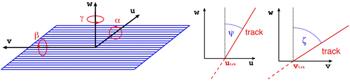
w u v γ α β u w track ψ utrk v w track ζ vtrkFigure 2. Sketch of a silicon strip module showing the axes of its local coordinate system, u, v, and w, and the respective local rotationsa, b, g (left), together with illustrations of the local track angles y and z (right).
over-noise ratio and a longer integration time, ideal for collecting cosmic ray tracks that appear at random times, but not suitable for the high bunch-crossing frequency of the LHC. Therefore, the strip tracker is operated in deconvolution mode when recording data during the LHC operation. The calibration and time synchronization of the strip modules are optimized for the two operation modes separately.
A local right-handed coordinate system is defined for each module with the origin at the
ge-ometric centre of the active area of the module. As illustrated in the left panel of figure2, the
u-axis is defined along the more precisely measured coordinate of the module (typically along the azimuthal direction in the global system), the v-axis orthogonal to the u-axis and in the module plane, pointing away from the readout electronics, and the w-axis normal to the module plane. The origin of the w-axis is in the middle of the module thickness. For the pixel system, u is chosen or-thogonal to the magnetic field, i.e. in the global rj direction in the BPIX and in the radial direction in the FPIX. The v-coordinate is perpendicular to u in the sensor plane, i.e. along global z in the BPIX and at a small angle to the global rj direction in the FPIX. The angles a, b, and g indicate right-handed rotations about the u-, v-, and w-axes, respectively. As illustrated in the right panel of
figure2, the local track angley (z) with respect to the module normal is defined in the u-w (v-w)
plane.
3 Global position and orientation of the tracker
While the track based internal alignment (see section4) mainly adjusts the positions and angles of
the tracker modules relative to each other, it cannot ascertain the absolute position and orientation of the tracker. Survey measurements of the TOB, as the largest single sub-component, are thus used to determine its shift and rotation around the beam axis relative to the design values. The other sub-components are then aligned relative to the TOB by means of the track based internal alignment procedure. The magnetic field of the CMS solenoid is to good approximation parallel to the z-axis. The orientation of the tracker relative to the magnetic field is of special importance, since the correct parameterisation of the trajectory in the reconstruction depends on it. This global orientation is
described by the anglesqx andqy, which correspond to rotations of the whole tracker around the
x- and y-axes defined in the previous section. Uncorrected overall tilts of the tracker relative to the magnetic field could result in biases of the reconstructed parameters of the tracks and the measured masses of resonances inferred from their charged daughter particles. Such biases would be hard
2014 JINST 9 P06009
to disentangle from the other systematic effects addressed in section4.4. It is therefore essential
to determine the global tracker tilt angles prior to the overall alignment correction, because the latter might be affected by a wrong assumption on the magnetic field orientation. It is not expected that tilt angles will change significantly with time, hence one measurement should be sufficient for many years of operation. The tilt angles have been determined with the 2010 CMS data, and they have been used as the input for the internal alignment detailed in subsequent sections of this article. A repetition of the procedure with 2011 data led to compatible results.
The measurement of the tilt angles is based on the study of overall track quality as a function of
theqxandqyangles. Any non-optimal setting of the tilt angles will result, for example, in incorrect
assumptions on the transverse field components relative to the tracker axis. This may degrade the
observed track quality. The tilt anglesqxandqyare scanned in appropriate intervals centred around
zero. For each set of values, the standard CMS track fit is applied to the whole set of tracks, and an
overall track quality estimator is determined. The track quality is estimated by the totalc2of all the
fitted tracks, c2. As cross-checks, two other track quality estimators are also studied: the mean
normalised trackc2per degree of freedom, hc2/N
dofi, and the mean p value, hP(c2,Ndof)i, which
is the probability of thec2to exceed the value obtained in the track fit, assuming ac2distribution
with the appropriate number of degrees of freedom. All methods yield similar results; remaining small differences are attributed to the different relative weight of tracks with varying number of hits and the effect of any remaining outliers.
Events are considered if they have exactly one primary vertex reconstructed by using at least four tracks, and a reconstructed position along the beam line within ±24 cm of the nominal centre of the CMS detector. Tracks are required to have at least ten reconstructed hits and a pseudorapidity of |h| < 2.5. The track impact parameter with respect to the primary vertex must be less than 0.15 cm (2 cm) in the transverse (longitudinal) direction. For the baseline analysis that provides the central values, the transverse momentum threshold is set to 1GeV/c; alternative values of 0.5 and
2GeV/c are used to check the stability of the results. Only tracks withc2/N
dof<4 are selected in
order to reject those with wrongly associated hits. For each setting of the tilt angles, each track is
refitted by using a full 3D magnetic field model [19,20] that also takes tangential field components
into account. This field model is based on measurements obtained during a dedicated mapping
operation with Hall and NMR probes [21].
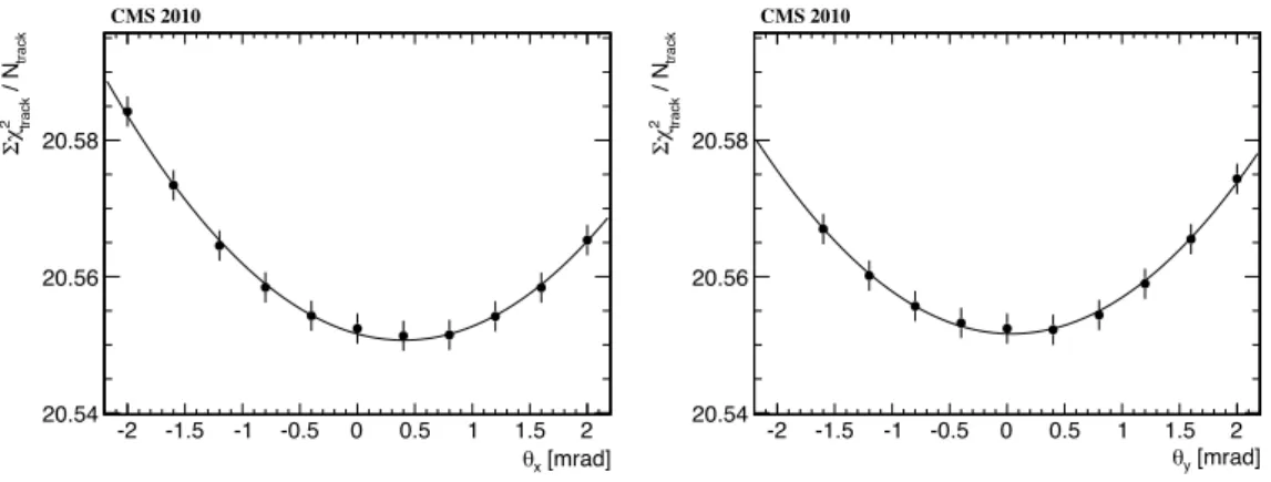
Each tilt angle is scanned at eleven settings in the range ±2 mrad. The angle of correct
align-ment is derived as the point of maximum track quality, corresponding to minimum totalc2,
deter-mined by a least squares fit with a second-order polynomial function. The dependence of the total
c2divided by the number of tracks on the tilt anglesq
xandqyis shown in figure3.
In each plot, only one angle is varied, while the other remains fixed at 0. The second-order polynomial fit describes the functional dependence very well. There is no result for the scan point
atqy= 2 mrad, because this setting is outside the range allowed by the track reconstruction
pro-gramme. While theqydependence is symmetric with a maximum nearqy⇡ 0, the qxdependence is
shifted towards positive values, indicating a noticeable vertical downward tilt of the tracker around the x-axis with respect to the magnetic field. On an absolute scale, the tilt is small, but nevertheless
visible within the resolution of beam line tilt measurements [15].
Figure4shows the resulting values ofqxandqy for five intervals of track pseudorapidity, for
2014 JINST 9 P06009
[mrad] x θ -2 -1.5 -1 -0.5 0 0.5 1 1.5 2 track / N track 2 χ Σ 20.54 20.56 20.58 CMS 2010 [mrad] y θ -2 -1.5 -1 -0.5 0 0.5 1 1.5 2 track / N track 2 χ Σ 20.54 20.56 20.58 CMS 2010Figure 3. Dependence of the total c2of the track fits, divided by the number of tracks, on the assumed
qx(left) andqy(right) tilt angles for |h| < 2.5 and pT>1GeV/c. The error bars are purely statistical and
correlated point-to-point because the same tracks are used for each point.
η -2 -1 0 1 2 [mrad] opt x,y θ -0.2 0 0.2 0.4 0.6 0.8 η -2 -1 0 1 2 [mrad] opt x,y θ -0.2 0 0.2 0.4 0.6 0.8 x θ y θ CMS 2010 Data η -2 -1 0 1 2 [mrad] opt x,y θ -0.2 0 0.2 0.4 0.6 0.8 η -2 -1 0 1 2 [mrad] opt x,y θ -0.2 0 0.2 0.4 0.6 0.8 x θ y θ CMS Simulation MC (no misalignment)
Figure 4. Tracker tilt angles qx(filled circles) andqy(hollow triangles) as a function of track pseudorapidity.
The left plot shows the values measured with the data collected in 2010; the right plot has been obtained from simulated events without tracker misalignment. The statistical uncertainty is typically smaller than the symbol size and mostly invisible. The outer error bars indicate the RMS of the variations which are observed when varying several parameters of the tilt angle determination. The shaded bands indicate the margins of ±0.1 mrad discussed in the text.
distance corresponding to a one unit increase of the total c2; they are at most of the order of the
symbol size and thus hardly visible. The outer error bars show the root mean square (RMS) of the
changes observed in the tilt angle estimates when changing the track quality estimators and the pT
threshold. The right plot shows the results of the method applied to simulated events without any tracker misalignment. They are consistent with zero tilt within the systematic uncertainty. The vari-ations are smaller in the central region within |h| < 1.5, and they are well contained within a margin of ±0.1 mrad, which is used as a rough estimate of the systematic uncertainty of this method. The
left plot in figure4 shows the result obtained from data; the qx values are systematically shifted
by ⇡0.3 mrad, while the qy values are close to zero. The nominal tilt angle values used as
align-ment constants are extracted from the centralh region of figure4(left) as qx= (0.3 ± 0.1) mrad
andqy= (0 ± 0.1) mrad, thus eliminating an important potential source of systematic alignment
uncertainty. These results represent an important complementary step to the internal alignment procedure described in the following sections.
2014 JINST 9 P06009
4 Methodology of track based internal alignment
Track-hit residual distributions are generally broadened if the assumed positions of the silicon modules used in track reconstruction differ from the true positions. Therefore standard alignment algorithms follow the least squares approach and minimise the sum of squares of normalised
resid-uals from many tracks. Assuming the measurements mi j, i.e. usually the reconstructed hit positions
on the modules, with uncertaintiessi j are independent, the minimised objective function is
c2(p,q) =tracks
Â
j measurementsÂ
i ✓mi j fi j(p,qj) si j ◆2 , (4.1)where fi jis the trajectory prediction of the track model at the position of the measurement,
depend-ing on the geometry (p) and track (qj) parameters. An initial geometry descriptionp0 is usually
available from design drawings, survey measurements, or previous alignment results. This can be
used to determine approximate track parametersqj0. Since alignment corrections can be assumed
to be small, fi j can be linearised around these initial values. Minimisingc2after the linearisation
leads to the normal equations of least squares. These can be expressed as a linear equation system
Ca = b with aT = ( p, q), i.e. the alignment parameters p and corrections to all parameters
of all n used tracks qT = ( q
1, . . . , qn). If the alignment corrections are not small, the linear
approximation is of limited precision and the procedure has to be iterated.
For the alignment of the CMS tracker a global-fit approach [22] is applied, by using the
MILLEPEDEII program [23]. It makes use of the special structure ofC that facilitates, by means
of block matrix algebra, the reduction of the large system of equationsCa = b to a smaller one for
the alignment parameters only,
C0 p = b0. (4.2)
HereC0 andb0 sum contributions from all tracks. To deriveb0, the solutions q
j of the track fit
equationsCj qj= bjare needed. ForC0, also the covariance matricesCj1have to be calculated.
The reduction of the matrix size from C to C0 is dramatic. For 107 tracks with on average 20
parameters and 105 alignment parameters, the number of matrix elements is reduced by a factor
larger than 4 ⇥ 106. Nevertheless, no information is lost for the determination of the alignment
parameters p.
The following subsections explain the track and alignment parameters q and p that are
used for the CMS tracker alignment. Then the concept of a hierarchical and differential alignment by using equality constraints is introduced, followed by a discussion of “weak modes” and how
they can be avoided. The section closes with the computing optimisations needed to make MILLE
-PEDEII a fast tool with modest computer memory needs, even for the alignment of the CMS tracker
with its unprecedented complexity. 4.1 Track parameterisation
In the absence of material effects, five parameters are needed to describe the trajectory of a charged particle in a magnetic field. Traversing material, the particle experiences multiple scattering, mainly due to Coulomb interactions with atomic nuclei. These effects are significant in the CMS tracker, i.e. the particle trajectory cannot be well described without taking them into account in the track
2014 JINST 9 P06009
model. This is achieved in a rigorous and efficient way as explained below in this section,
repre-senting an improvement compared to previous MILLEPEDEII alignment procedures [10, 11,13]
for the CMS silicon tracker, which ignored correlations induced by multiple scattering.
A rigorous treatment of multiple scattering can be achieved by increasing the number of track parameters to npar= 5+2nscat, e.g. by adding two deflection angles for each of the nscatthin
scatter-ers travscatter-ersed by the particle. For thin scatterscatter-ers, the trajectory offsets induced by multiple scattering can be ignored. If a scatterer is thick, it can be approximately treated as two thin scatterers. The distributions of these deflection angles have mean values of zero. Their standard deviations can be estimated by using preliminary knowledge of the particle momentum and of the amount of ma-terial crossed. This theoretical knowledge is used to extend the list of measurements, originally containing all the track hits, by “virtual measurements”. Each scattering angle is virtually mea-sured to be zero with an uncertainty corresponding to the respective standard deviation. These virtual measurements compensate for the degrees of freedom introduced in the track model by increasing its number of parameters. For cosmic ray tracks this complete parameterisation often leads to npar>50. Since in the general case the effort to calculateCj1 is proportional to n3par, a
significant amount of computing time would be spent to calculate C 1
j and thus C0 andb0. The
progressive Kalman filter fit, as used in the CMS track reconstruction [43], avoids the n3
par scaling
by a sequential fit procedure, determining five track parameters at each measurement. However,
the Kalman filter does not provide the full (singular) covariance matrixC 1
j of these parameters as
needed in a global-fit alignment approach. As shown in [24], the Kalman filter fit procedure can be
extended to provide this covariance matrix, but since MILLEPEDEII is designed for a simultaneous
fit of all measurements, another approach is followed here.
The general broken lines (GBL) track refit [25,26] that generalises the algorithm described in
ref. [27], avoids the n3
par scaling for calculatingCj1by defining a custom track parameterisation.
The parameters areqj= (Dqp,u1, . . . ,u(nscat+2)), whereD
q
p is the change of the inverse momentum
multiplied by the particle charge and ui are the two-dimensional offsets to an initial reference
trajectory in local systems at each scatterer and at the first and last measurement. All parameters
exceptDq
p influence only a small part of the track trajectory. This locality of all track parameters
(but one) results inCj being a bordered band matrix with band width m 5 and border size b = 1,
i.e. the matrix elements ckl
j are non-zero only for k b, l b or |k l| m. By means of root-free
Cholesky decomposition (Cband
j = LDLT) of the band partCbandj into a diagonal matrixD and a unit
left triangular band matrixL, the effort to calculate C 1
j andqj is reduced toµ n2par· (m + b) and
µ npar· (m + b)2, respectively. This approach saves a factor of 6.5 in CPU time for track refitting in
MILLEPEDEII for isolated muons (see section5) and of 8.4 for cosmic ray tracks in comparison
with an (equivalent) linear equation system with a dense matrix solved by inversion.
The implementation of the GBL refit used for the MILLEPEDEII alignment of the CMS tracker
is based on a seed trajectory derived from the position and direction of the track at its first hit as resulting from the standard Kalman filter track fit. From the first hit, the trajectory is propagated taking into account magnetic-field inhomogeneities, by using the Runge-Kutta technique as
de-scribed in [43], and the average energy loss in the material as for muons. As in the CMS Kalman
filter track fit, all traversed material is assumed to coincide with the silicon measurement planes
that are treated as thin scatterers. The curvilinear frame defined in [28] is chosen for the local
2014 JINST 9 P06009
r u -1 -0.5 0 0.5 1 r v -1 -0.5 0 0.5 1 w -0.2 0 0.2 0.4 0.6 - 1/3 2 r : u 20 w r u -1 -0.5 0 0.5 1 r v -1 -0.5 0 0.5 1 w -1 -0.5 0 0.5 1 r v ⋅ r : u 11 w r u -1 -0.5 0 0.5 1 r v -1 -0.5 0 0.5 1 w -0.2 0 0.2 0.4 0.6 - 1/3 2 r : v 02 wFigure 5. The three two-dimensional second-order polynomials to describe sensor deviations from the flat plane, illustrated for sagittae w20= w11= w02= 1.
the local systems uses Jacobians assuming a locally constant magnetic field between them [28].
To further reduce the computing time, two approximations are used in the standard processing: material assigned to stereo and rj modules that are mounted together is treated as a single thin scatterer, and the Jacobians are calculated assuming the magnetic field ~B to be parallel to the z-axis in the limit of weak deflection, |~B|
p ! 0. This leads to a band width of m = 4 in the matrix Cj.
4.2 Alignment parameterisation
To first approximation, the CMS silicon modules are flat planes. Previous alignment approaches in CMS ignored possible deviations from this approximation and determined only corrections to the initial module positions, i.e. up to three shifts (u, v, w) and three rotations (a, b, g). However, tracks with large angles of incidence relative to the silicon module normal are highly sensitive to the exact positions of the modules along their w directions and therefore also to local w variations if the modules are not flat. These local variations can arise from possible curvatures of silicon sensors and, for strip modules with two sensors in a chain, from their relative misalignment. In fact, sensor curvatures can be expected because of tensions after mounting or because of single-sided silicon processing as for the strip sensors. The specifications for the construction of the sensors
required the deviation from perfect planarity to be less than 100µm [1]. To take into account such
deviations, the vector of alignment parameters p is extended to up to nine degrees of freedom
per sensor instead of six per module. The sensor shape is parameterised as a sum of products of modified (orthogonal) Legendre polynomials up to the second order where the constant and linear
terms are equivalent to the rigid body parameters w,a and b:
w(ur,vr) = w
+ w10· ur + w01· vr
+ w20· (u2r 1/3) + w11· (ur· vr) + w02· (v2r 1/3).
(4.3)
Here ur2 [ 1,1] (vr2 [ 1,1]) is the position on the sensor in the u- (v-) direction, normalised
to its width lu (length lv). The coefficients w20, w11 and w02 quantify the sagittae of the sensor
curvature as illustrated in figure5. The CMS track reconstruction algorithm treats the hits under
the assumption of a flat module surface. To take into account the determined sensor shapes, the
2014 JINST 9 P06009
( w(ur,vr) · tanz), respectively. Here the track angle from the sensor normal y (z) is defined in
the u-w (v-w) plane (figure2), and the track predictions are used for urand vr.
To linearise the track-model prediction fi j, derivatives with respect to the alignment parameters
have to be calculated. If fi j is in the local u (v) direction, denoted as fu( fv) in the following, the
derivatives are 0 B B B B B B B B B B B B B B B B B B B B B @ ∂ fu ∂u ∂ f∂uv ∂ fu ∂v ∂ f∂vv ∂ fu ∂w ∂ f∂wv ∂ fu ∂w10 ∂ fv ∂w10 ∂ fu ∂w01 ∂ fv ∂w01 ∂ fu ∂g0 ∂ f∂gv0 ∂ fu ∂w20 ∂ fv ∂w20 ∂ fu ∂w11 ∂ fv ∂w11 ∂ fu ∂w02 ∂ fv ∂w02 1 C C C C C C C C C C C C C C C C C C C C C A = 0 B B B B B B B B B B B B B B B B B B B B B @ 1 0 0 1 tany tanz ur· tany ur· tanz vr· tany vr· tanz vrlv/(2s) urlu/(2s) (u2 r 1/3) · tany (u2r 1/3) · tanz ur· vr· tany ur· vr· tanz (v2 r 1/3) · tany (v2r 1/3) · tanz 1 C C C C C C C C C C C C C C C C C C C C C A . (4.4)
Unlike the parameterisation used in previous CMS alignment procedures [29], the coefficients
of the first order polynomials w01=l2v·tana and w10= 2lu·tanb are used as alignment parameters
instead of the angles. This ensures the orthogonality of the sensor surface parameterisation. The in-plane rotationg is replaced by g0= s·g with s =lu+lv
2 . This has the advantage that all parameters
have a length scale and their derivatives have similar numerical size.
The pixel modules provide uncorrelated measurements in both u and v directions. The strips of the modules in the TIB and TOB are parallel along v, so the modules provide measurements only in the u direction. For TID and TEC modules, where the strips are not parallel, the hit reconstruction provides highly correlated two-dimensional measurements in u and v. Their covariance matrix is diagonalised and the corresponding transformation applied to the derivatives and residuals as well. The measurement in the less precise direction, after the diagonalisation, is not used for the alignment.
4.3 Hierarchical and differential alignment by using equality constraints
The CMS tracker is built in a hierarchical way from mechanical substructures, e.g. three BPIX half-layers form each of the two BPIX half-shells. To treat translations and rotations of these
sub-structures as a whole, six alignment parameters pl for each of the considered substructures can
be introduced. The derivatives of the track prediction with respect to these parameters, d fu/v/d pl,
are obtained from the six translational and rotational parameters of the hit sensor psby coordinate
transformation with the chain rule
d fu/v d pl = d ps d pl · d fu/v d ps, (4.5) where d ps
d pl is the 6 ⇥ 6 Jacobian matrix expressing the effect of translations and rotations of the
2014 JINST 9 P06009
These large-substructure parameters are useful in two different cases. If the track sample is too small for the determination of the large number of alignment parameters at module level, the alignment can be restricted to the much smaller set of parameters of these substructures. In addition they can be used in a hierarchical alignment approach, simultaneously with the alignment parameters of the sensors. This has the advantage that coherent misplacements of large structures in directions of the non-sensitive coordinate v of strip sensors can be taken into account.
This hierarchical approach introduces redundant degrees of freedom since movements of the large structures can be expressed either by their alignment parameters or by combinations of the parameters of their components. These degrees of freedom are eliminated by using linear equality constraints. In general, such constraints can be formulated as
Â
i
ciDpi= s, (4.6)
where the index i runs over all the alignment parameters. In MILLEPEDEII these constraints are
implemented by extending the matrix equation (4.2) by means of Lagrangian multipliers. In the
hierarchical approach, for each parameterDpl of the larger structure one constraint with s = 0 has
to be applied and then all constraints for one large structure form a matrix equation,
components
Â
i d ps,i d pl 1 · pi= 0, (4.7)where ps,iare the shift and rotation parameters of component i of the large substructure.
Simi-larly, the technique of equality constraints is used to fix the six undefined overall shifts and rotations of the complete tracker.
The concept of “differential alignment” means that in one alignment step some parameters are treated as time-dependent while the majority of the parameters stays time-independent. Time
dependence is achieved by replacing an alignment parameterDpt in the linearised form of
equa-tion (4.1) by several parameters, each to be used for one period of time only. This method allows
the use of the full statistical power of the whole dataset for the determination of parameters that are stable with time, without neglecting the time dependence of others. This is especially useful in conjunction with a hierarchical alignment: the parameters of larger structures can vary with time, but the sensors therein are kept stable relative to their large structure.
4.4 Weak modes
A major difficulty of track based alignment arises if the matrix C0 in equation (4.2) is
ill-condi-tioned, i.e. singular or numerically close to singular. This can result from linear combinations of the alignment parameters that do not (or only slightly) change the track-hit residuals and thus
the overallc2( p, q) in equation (4.1), after linearisation of the track model f
i j. These linear
combinations are called “weak modes” since the amplitudes of their contributions to the solution are either not determinable or only barely so.
Weak modes can emerge if certain coherent changes of alignment parameters p can be
compensated by changes of the track parameters q. The simplest example is an overall shift of
the tracker that would be compensated by changes of the impact parameters of the tracks. For that reason the overall shift has to be fixed by using constraints as mentioned above. Other weak modes
2014 JINST 9 P06009
discussed below influence especially the transverse momenta of the tracks. A specific problem is
that even very small biases in the track model fi j can lead to a significant distortion of the tracker
if a linear combination of the alignment parameters is not well determined by the data used in
equation (4.1). As a result, weak modes contribute significantly to the systematic uncertainty of
kinematic properties determined from the track fit.
The range of possible weak modes depends largely on the geometry and segmentation of the detector, the topology of the tracks used for alignment, and on the alignment and track parame-ters. The CMS tracker has a highly segmented detector geometry with a cylindrical layout within a solenoidal magnetic field. If aligned only with tracks passing through the beam line, the
charac-teristic weak modes can be classified in cylindrical coordinates, i.e. by module displacementsDr,
Dz, and Dj as functions of r, z, and j [30]. To control these weak modes it is crucial to include
ad-ditional information in equation (4.1), e.g. by combining track sets of different topological variety
and different physics constraints by means of
• cosmic ray tracks that break the cylindrical symmetry,
• straight tracks without curvature, recorded when the magnetic field is off, • knowledge about the production vertex of tracks,
• knowledge about the invariant mass of a resonance whose decay products are observed as tracks.
Earlier alignment studies [13] have shown that the usage of cosmic ray tracks is quite effective
in controlling several classes of weak modes. However, for some types of coherent deformations of the tracker the sensitivity of an alignment based on cosmic ray tracks is limited. A prominent
example biasing the track curvaturek µ q
pT (with q being the track charge) is a twist deformation
of the tracker, in which the modules are moved coherently inj by an amount directly proportional
to their longitudinal position (Dj = t · z). This has been studied extensively in [31]. Other
poten-tial weak modes are the off-centring of the barrel layers and endcap rings (sagitta), described by
(Dx,Dy) = s ·r·(sinjs,cosjs), and a skew, parameterised asDz = w ·sin(j +jw). Heres and w
denote the amplitudes of the sagitta and skew weak modes, whereasjs andjw are their azimuthal
phases.
As a measure against weak modes that influence the track momenta, such as a twist deforma-tion, information on the mass of a resonance decaying into two charged particles is included in the alignment fit with the following method. A common parameterisation for the two trajectories of the
particles produced in the decay is defined as in [32]. Instead of 2·5 parameters (plus those
account-ing for multiple scatteraccount-ing), the nine common parameters are the position of the decay vertex, the momentum of the resonance candidate, two angles defining the direction of the decay products in the rest-frame of the resonance, and the mass of the resonance. The mean mass of the resonance is added as a virtual measurement with an uncertainty equal to the standard deviation of its invariant mass distribution. Mean and standard deviation are estimated from the distribution of the invariant mass in simulated decays, calculated from the decay particles after final-state radiation. In the sum
on the right hand side of equation (4.1), the two individual tracks are replaced by the common fit
2014 JINST 9 P06009
approach to include resonance mass information in the alignment fit implies an implementation of a vertex constraint as well, since the coordinates of the decay vertex are parameters of the combined fit object and thus force the tracks to a common vertex.
The dependence of the reconstructed resonance mass M on the sizet of a twist deformation
can be shown to follow
∂M2 ∂t = ✓M2 p+ ∂ p+ ∂t + M2 p ∂ p ∂t ◆ =2M2 Bz p + z pz . (4.8)
Here Bzdenotes the strength of the solenoidal magnetic field along the z-axis, p+(p ) and p+z (pz)
are the momentum and its longitudinal component of the positively (negatively) charged particle,
respectively. Equation (4.8) shows that the inclusion of a heavy resonance such as the Z boson in
the alignment procedure is more effective for controlling the twist than the J/y and ° quarkonia,
since at the LHC the decay products of the latter are usually boosted within a narrow cone, and the difference of their longitudinal momenta is small. The decay channel of Z to muons is particularly
useful because the high-pT muons are measured precisely and with high efficiency by the CMS
detector. The properties of the Z boson are predicted by the Standard Model and have been
char-acterised experimentally very well at the LHC [33,34] and in past experiments [35]. This allows
the muonic decay of the Z boson to be used as a standard reference to improve the ability of the alignment procedure to resolve systematic distortions, and to verify the absence of any bias on the track reconstruction.
Under certain conditions, equality constraints can be utilised against a distortion in the
start-ing geometryp0induced by a weak mode in a previous alignment attempt. The linear combination
of the alignment parameters corresponding to the weak mode and the amplitude of the distortion in the starting geometry have to be known. In this case, a constraint used in a further alignment step can remove the distortion, even if the data used in the alignment cannot determine the
am-plitude. If, for example, each aligned object i is, compared to its true position, misplaced in j
according to a twist t with reference point z0 (Dji=t · (zi z0)), this constraint takes the form
ÂiÂj∂Dp∂Dji ji Âk(z(zikz0z)0)2Dpi j = t, where the sums over i and k include the aligned objects and the
sum over j includes their active alignment parametersDpi j.
4.5 Computing optimisation
The MILLEPEDE II program proceeds in a two-step approach. First, the standard CMS software
environment [5] is used to produce binary files containing the residuals mi j fi j, their dependence
on the parameters p and q of the linearised track model, the uncertainties si j, and labels
identifying the fit parameters. Second, these binary files are read by an experiment-independent
program that sets up equation (4.2), extends it to incorporate the Lagrangian multipliers to
imple-ment constraints, and solves it, e.g. by the iterative MINRESalgorithm [36]. In contrast to other fast
algorithms for solving large matrix equations, MINRESdoes not require a positive definite matrix,
and because of the Lagrangian multipliersC0is indefinite. Since the convergence speed of MINRES
depends on the eigenvalue spectrum of the matrixC0, preconditioning is used by multiplying
equa-tion (4.2) by the inverse of the diagonal of the matrix. The elements of the symmetric matrixC0
in general require storage in double precision while they are summed. For the 200 000 alignment parameters used in this study, this would require 160 GB of RAM. Although the matrix is rather
2014 JINST 9 P06009
sparse and only non-zero elements are stored, the reduction is not sufficient. High alignment pre-cision also requires the use of many millions of tracks of different topologies that are fitted several
times within MILLEPEDEII, leading to a significant contribution to the CPU time. To cope with
the needs of the CMS tracker alignment described in this article, the MILLEPEDEII program has
been further developed, in particular to reduce the computer memory needs, to enlarge the number
of alignment parameters beyond what was used in [13], and to reduce the processing time. Details
are described in the following.
Since the non-zero matrix elements are usually close to each other in the matrix, further reduc-tion of memory needs is reached by bit-packed addressing of non-zero blocks in a row. In addireduc-tion, some matrix elements sum contributions of only a few tracks, e.g. cosmic ray tracks from rare directions. For these elements, single precision storage is sufficient.
Processing time is highly reduced in MILLEPEDE II by shared-memory parallelisation by
means of the Open Multi-Processing (OPENMPR) package [37] for the most computing intensive
parts like the product of the huge matrixC0with a vector for MINRES, the track fits for the
calcula-tion of qjandCj1, and the construction ofC0from those. Furthermore, bordered band matrices
Cj are automatically detected and root-free Cholesky decomposition is applied subsequently (see
section4.1).
Reading data from local disk and memory access are further potential bottlenecks. The band
structure of Cj that is due to the GBL refit and the approximations in the track model (see
sec-tion4.1) also aim to alleviate the binary file size. To further reduce the time needed for reading,
MILLEPEDEII reads compressed input and caches the information of many tracks to reduce the
number of disk accesses.
5 Strategy of the internal alignment of the CMS tracker
In general, the tracker has been sufficiently stable throughout 2011 to treat alignment parameters
as constant in time. The stability of large structures has been checked as described in section 6.
An exception to this stability is the pixel detector whose movements have been carefully monitored and are then treated as described below. Validating the statistical alignment precision by means of
the methods of section7shows no need to have a further time dependent alignment at the single
module parameter level. Also, calibration parameters influence the reconstructed position of a hit on a module. These parameters account for the Lorentz drift of the charge carriers in the silicon due to the magnetic field and for the inefficient collection of charge generated near the back-plane of
strip sensors if these are operated in deconvolution mode [43]. Nevertheless, for 2011 data there is
no need to integrate the determination of calibration parameters into the alignment procedure. The hit position effect of any Lorentz drift miscalibration is compensated by the alignment corrections and as long as the Lorentz drift is stable with time, the exact miscalibration has no influence on the statistical alignment precision. Also the back-plane correction has only a very minor influence. No significant degradation of the statistical alignment precision with time has been observed.
Given this stability, the 2011 alignment strategy of the CMS tracker consists of two steps;
both apply the techniques and tools described in section 4. The first step uses data collected in
2011 up to the end of June, corresponding to an integrated luminosity of about 1fb 1. This step
2014 JINST 9 P06009
vertex information. The details are described in the rest of this section. The second step treats the four relevant movements of the pixel detector after the end of June, identified with the methods of
section6.2. Six alignment parameters for each BPIX layer and FPIX half-disk are redetermined by
a stand-alone alignment procedure, keeping their internal structures unchanged and the positions of the strip modules constant.
Tracks from several data sets are used simultaneously in the alignment procedure. Hit and
track reconstruction are described in [43] and the following selection criteria are applied:
• Isolated muons: global muons [16] are reconstructed in both the tracker and the muon
system. They are selected if their number of hits Nhitin the tracker exceeds nine (at least one
of which is in the pixel detector, Nhit(pixel) 1), their momenta p are above 8GeV/c (in order
to minimise the effects of Multiple Coulomb scattering), and their transverse momenta pTare
above 5GeV/c. Their distancesDR =p(Dj)2+ (Dh)2from the axes of jets reconstructed in
the calorimeter and fulfilling pT>40GeV/c have to be larger than 0.1. This class of events is
populated mainly by muons belonging to leptonic W -boson decays and about 15 million of these tracks are used for the alignment.
• Tracks from minimum bias events: a minimum bias data sample is selected online with a combination of triggers varying with pileup conditions, i.e. the mean number of additional collisions, overlapping to the primary one, within the same bunch crossing (on average 9.5 for the whole 2011 data sample). These triggers are based, for example, on pick-up sig-nals indicating the crossing of two filled proton bunches, sigsig-nals from the Beam Scintillator
Counters [1], or moderate requirements on hit and track multiplicity in the pixel detectors.
The offline track selection requires Nhit>7, p > 8GeV/c. Three million of these tracks are
used for alignment.
• Muons from Z-boson decays: events passing any trigger filter requesting two muons recon-structed online are used for reconstructing Z-boson candidates. Two muons with opposite
charge must be identified as global muons and fulfil the requirement Nhit>9 (Nhit(pixel)
1). Their transverse momenta must exceed pT >15GeV/c and their distances to jets
re-constructed in the calorimeter DR > 0.2. The invariant mass of the reconstructed dimuon
system must lie in the range 85.8 < Mµ+µ <95.8GeV/c2, in order to obtain a pure sample
of Z-boson candidates. The total number of such muon pairs is 375 000.
• Cosmic ray tracks: cosmic ray events used in the alignment were recorded with the strip tracker operated both in peak and deconvolution modes. Data in peak mode were recorded in a dedicated cosmic data taking period before the restart of the LHC operations in 2011 and during the beam-free times between successive LHC fills. In addition, cosmic ray data were taken in deconvolution mode both during and between LHC fills, making use of a dedicated trigger selecting cosmic ray tracks passing through the tracker barrel. In total 3.6 million
cosmic ray tracks with p > 4GeV/c and Nhit>7 are used, where about half of the sample
has been collected with the strip tracker operating in peak mode, while the other half during operations in deconvolution mode.
For all the data sets, basic quality criteria are applied on the hits used in the track fit and on the tracks themselves:
2014 JINST 9 P06009
• the signal-over-noise ratio of the strip hits must be higher than 12 (18) when the strip tracker records data in deconvolution (peak) mode;
• for pixel hits, the probability of the hit to match the expected shape of the charge cluster for
the given track parameters [38] must be higher than 0.001 (0.01) in the u (v) direction;
• for all hits, the angle between the track and the module surface must be larger than 10 (20 ) for tracks from proton-proton collisions (cosmic rays) to avoid a region where the estimates of the hit position and uncertainty are less reliable;
• to ensure a reliable determination of the polar track angle, q, tracks have to have at least two hits in pixel or stereo strip modules;
• tracks from proton-proton collisions have to satisfy the “high-purity” criteria [14,43] of the
CMS track reconstruction code;
• in the final track fit within MILLEPEDEII, tracks are rejected if theirc2value is larger than
the 99.87% quantile (corresponding to three standard deviations) of thec2 distribution for
the number of degrees of freedom Ndofof the track.
The tracker geometry, as determined by the alignment with the 2010 data [31], is the starting
point of the 2011 alignment procedure. In general, for each sensor all nine parameters are included in the alignment procedure. Exceptions are the v coordinate for strip sensors since it is orthogonal
to the measurement direction, and the surface parameterisation parameters w10, w01, w20, w11,
w02 for the FPIX modules. The latter exception is due to their small size and smaller sensitivity
compared to the other subdetectors, caused by the smaller spread of track angles with respect to the module surface.
The hierarchical alignment approach discussed in section4.3is utilised by introducing
param-eters for shifts and rotations of half-barrels and end-caps of the strip tracker and of the BPIX layers and FPIX half-disks. For the parameters of the BPIX layers and FPIX half-disks the differential alignment is used as well. The need for nine time periods (including one for the cosmic ray data
before the LHC start) has been identified with the validation procedure of section6.2. The
param-eters for the six degrees of freedom of each of the two TOB half-barrels are constrained to have opposite sign, fixing the overall reference system.
Three approaches have been investigated to overcome the twist weak mode introduced in
sec-tion4.4. The first uses tracks from cosmic rays, recorded in 2010 when the magnetic field was off.
This successfully controls the twist, but no equivalent data were available in 2011. Second, the
twist has been measured in the starting geometry with the method of section9.2. An equality
con-straint has been introduced to compensate for it. While this method controls the twist, it does not
reduce the dependence of the muon kinematics on the azimuthal angle seen in sections9.1and9.2.
Therefore the final alignment strategy is based on the muons from Z-boson decays to include mass
information and vertex constraints in the alignment procedure as described in section4.4, with a
virtual mass measurement of Mµ+µ = 90.86 ± 1.86GeV/c2.
In total, more than 200 000 alignment parameters are determined in the common fit, by using 138 constraints. To perform this fit, 246 parallel jobs produce the compressed input files
2014 JINST 9 P06009
program. The total size of these files is 46.5 GB. The matrixC0 constructed from this by MILLE
-PEDE II contains 31% non-zero off-diagonal elements. With a compression ratio of 40% this fits
well into an affordable 32 GB of memory. The MINRES algorithm has been run four times with
increasingly tighter rejection of bad tracks. SinceC0is not significantly changed by this rejection,
it does not need to be recalculated after the first iteration. By means of eight threads on an IntelR
XeonR L5520 processor with 2.27 GHz, the CPU usage was 44:30 h with a wall clock time of only
9:50 h. This procedure has been repeated four times to treat effects from non-linearity: iterating the procedure is particularly important for eliminating the twist weak mode.
The same alignment procedure as used on real data was run on a sample of simulated tracks, prepared with the same admixture of track samples as in the recorded data. The geometry obtained in this way is characterised by a physics performance comparable to the one obtained with recorded data and can be used for comparisons with simulated events. This geometry is referred as the “realistic” misalignment scenario.
6 Monitoring of the large structures
A substantial fraction of the analyses in CMS use data reconstructed immediately after its acqui-sition (prompt reconstruction) for obtaining preliminary sets of results. Therefore, it is important to provide to the physics analyses the best possible geometry for use in the prompt reconstruction, immediately correcting any possible time-dependent large misalignment. Specifically, the position of the large structures in the pixel detector is relevant for the performance of b-tagging algorithms.
As described in [8], misalignment at the level of a few tens of microns can seriously affect the
b-tagging performance.
In order to obtain the best possible track reconstruction performance, the tracker geometry is carefully monitored as a function of time, so that corrections can be applied upon movements large enough to affect the reconstruction significantly. The CMS software and reconstruction frame-work accommodates time-dependent alignment and calibration conditions by “intervals of validity”
(IOV), which are periods during which a specific set of constants retain the same values [5]. While
the alignment at the level of the single modules needs data accumulated over substantial periods of time, the stability of the position of the large structures can be controlled with relatively small amounts of data or via a system of infrared lasers. The short data acquisition times required by these monitoring methods allow fast and frequent feedback to the alignment procedure. A system of laser beams is able to monitor the positions of a restricted number of modules in the silicon strip tracker. Movements of large structures in the pixel tracker can be detected with high precision with collision tracks by a statistical study of the primary-vertex residuals, defined as the distance be-tween the tracks and the primary vertex at the point of closest approach of the tracks to the vertex. All these techniques allow the monitoring of the position of the large structures on a daily basis.
This frequent monitoring, together with the fast turn-around of the alignment with MILLEPEDEII,
allows, if needed, the correction of large movements on the timescale of one day. 6.1 Monitoring of the strip tracker geometry
The CMS laser alignment system (LAS) [39] provides a source of alignment information
2014 JINST 9 P06009
of the silicon sensors that are used also for the standard track reconstruction (see figure1). The
laser optics are mounted on mechanical structures independent of those used to support the tracker. With this limited number of laser beams one can align large-scale structures such as the TOB, TIB, and both TECs. The mechanical accuracy of LAS components limits the absolute precision of this alignment method to ⇠50 µm in comparison to the alignment with tracks, which reaches better
than 10µm resolution (see section7), but the response time of the LAS is at the level of only a few
minutes. Within this margin of accuracy, the LAS measurement demonstrated very good stability of the strip detector geometry over the whole 2011 running period. This observation is confirmed by a dedicated set of alignments with tracks, where the dataset was divided into different time periods. No significant movements of the large structures of the silicon strip tracker were found. 6.2 Monitoring of the pixel detector geometry with tracks
The large number of tracks produced in a pp collision allows precise reconstruction of the
interac-tion vertices [15]. The resolution of the reconstructed vertex position is driven by the pixel detector
since it is the sub-structure that is closest to the interaction point and has the best hit resolution. The primary vertex residual method is based on the study the distance between the track and the vertex, the latter reconstructed without the track under scrutiny (unbiased track-vertex residual). Events
used in this analysis are selected online with minimum bias triggers as mentioned in section5. The
analysis uses only vertices with distances from the nominal interaction pointpx2
vtx+ y2vtx<2 cm
and |zvtx| < 24 cm in the transverse and longitudinal direction, respectively. The fit of the vertex
must have at least 4 degrees of freedom. For each of these vertices, the impact parameters are measured for tracks with:
• more than six hits in the tracker, of which at least two are in the pixel detector, • at least one hit in the first layer of the BPIX or the first disk of the FPIX, • pT>1GeV/c,
• c2/Ndofof the track smaller than 5.
The vertex position is recalculated excluding the track under scrutiny from the track collection.
A deterministic annealing clustering algorithm [40] is used in order to make the method robust
against pileup, as in the default reconstruction sequence.
The distributions of the unbiased track-vertex residuals in the transverse plane, ˜dxy, and in the
longitudinal direction, ˜dz, are studied in bins ofh and j of the track. Random misalignments of
the modules affect only the resolution of the unbiased track-vertex residual, increasing the width of the distributions, but without biasing their mean. Systematic movements of the modules will bias the distributions in a way that depends on the nature and size of the misalignment and the
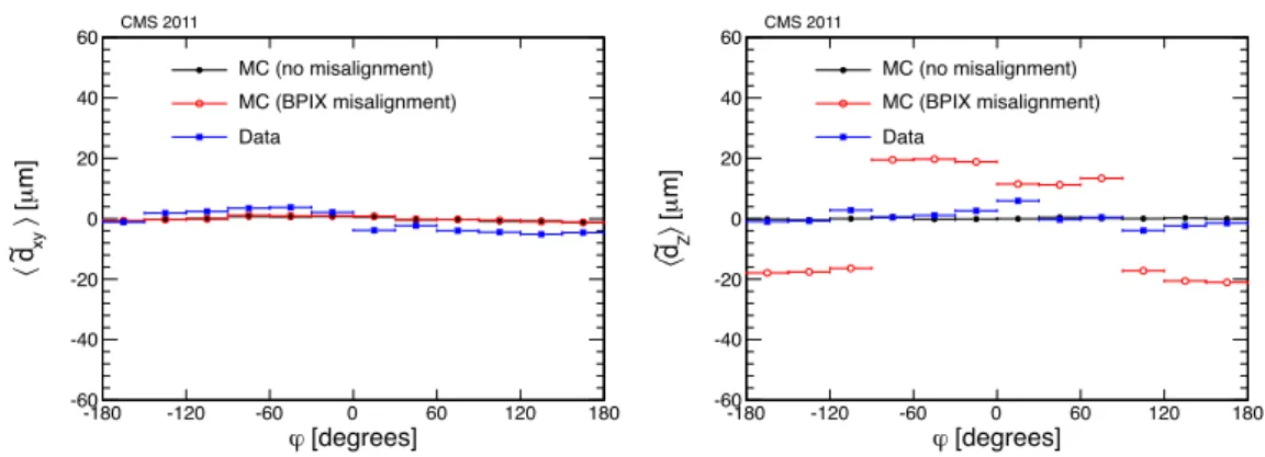
h and j of the selected tracks. As an example, the dependence of the means of the ˜dxy and ˜dz
distributions as a function of the azimuthal angle of the track is shown in figure6. The focus on
the j-dependence is motivated by the design of the BPIX, which is divided into one half-shell
with modules atj 2 [ p/2,p/2] and another with modules at j 2 [p/2,p] [ [ p, p/2]. Small
movements of the two half-shells are mechanically allowed by the mechanical design of the pixel detector. The observed movements have not been associated to a specific cause, although thermal
2014 JINST 9 P06009
[degrees] ϕ -180 -120 -60 0 60 120 180 m] µ [ 〉 xy d ~ 〈 -60 -40 -20 0 20 40 60 CMS 2011 MC (no misalignment) MC (BPIX misalignment) Data [degrees] ϕ -180 -120 -60 0 60 120 180 m] µ [ 〉 Z d ~ 〈 -60 -40 -20 0 20 40 60 CMS 2011 MC (no misalignment) MC (BPIX misalignment) DataFigure 6. Means of the distributions of the unbiased transverse (left) and longitudinal (right) track-vertex residuals as a function of the azimuthal angle of the track. Blue squares show the distribution obtained from about ten thousand minimum bias events recorded in 2011. Full black circles show the prediction by using a simulation with perfect alignment. Open red circles show the same prediction by using a geometry with the two BPIX half-shells shifted by 20µm in opposite z-directions in the simulation.
cycles executed on the pixel detector increase the chances that such movements will happen. As an example, the impact of a movement of one half-shell with respect to the other in the longitudinal
direction is shown by the open circles in figure6for a simulated sample of minimum bias events.
Such a movement is reflected in a very distinctive feature in the dependence of the mean of the ˜
dz distribution as a function of j. The size of the movement can be estimated as the average
bias in the two halves of the BPIX. The time dependence of this quantity in the 2011 data is
illustrated in figure7, which shows some discontinuities. Studies carried out on simulated data
show that the b-tagging performance is visibly degraded in the case of uncorrected shifts with
amplitude |Dz| > 20 µm [8]. For this reason, IOVs with different alignments of the pixel layers
are conservatively defined according to the boundaries of periods with steps of |Dz| larger than
10µm. The time-dependent alignment parameters of BPIX layers and FPIX half-disks during the
first eight IOVs (until end of June 2011) were determined in a single global fit. Within each time interval, the positions of the modules with respect to the structure were found not to need any further correction. Because of this, the positions of the pixel layers and half-disks were determined by a dedicated alignment procedure keeping the other hierarchies of the geometry unchanged. The aligned geometry performs well over the entire data-taking period, reducing the observed jumps in the expected way. Residual variations can be attributed to small misalignments with negligible impact on physics performance and to the resolution of the validation method itself.
7 Statistical accuracy of the alignment
A method for assessing the achieved statistical precision of the aligned positions in the sensitive direction of the modules has been successfully explored and adopted in the alignment of the CMS
tracker during commissioning with cosmic rays, described in [13]. The results from the validation
are based on isolated muon tracks with a transverse momentum of pT>40GeV/c and at least ten
hits in the tracker. The tracks are refitted with the alignment constants under study. Hit residuals are determined with respect to the track prediction, which is obtained without using the hit in
2014 JINST 9 P06009
Date 02/21 03/20 04/16 05/14 06/10 07/08 08/04 08/31 09/28 10/25 11/21 m] µ z [ ∆ -20 0 20 4060 Data (no realignment)
Data (after realignment) CMS 2011
Figure 7. Daily evolution of the relative longitudinal shift between the two half-shells of the BPIX as measured with the primary-vertex residuals. The open circles show the shift observed by using prompt reconstruction data in 2011. The same events were reconstructed again after the 2011 alignment campaign, which accounts for the major changes in the positions of the half-shells (shown as filled squares). Dashed vertical lines indicate the chosen IOVs boundaries where a different alignment of the pixel layers has been performed.
question to avoid any correlation between hit and track. From the distribution of the unbiased hit residuals in each module, the median is taken and histogrammed for all modules in a detector subsystem. The median is relatively robust against stochastic effects from multiple scattering, and thus the distribution of the medians of residuals (DMR) is a measure of the alignment accuracy. Only modules with at least 30 entries in their distribution of residuals are considered.
The addition of proton-proton collision events leads to a huge increase of the number of tracks available for the alignment, especially for the innermost parts of the tracker. Compared to the
alignment with cosmic rays alone [13], considerable improvements are consequently observed in
the pixel tracker, especially in the endcaps. The corresponding DMR are shown in the figure 8,
separately for the u and v coordinates; for both pixel tracker barrel (BPIX) and endcap (FPIX)
detectors, the RMS is well below 3µm in both directions, compared to about 13 µm for the endcaps
in the cosmic ray-only alignment. These numbers are identical or at most only slightly larger than
those obtained in simulation without any misalignment, which are below 2µm and thus far below
the expected hit resolution. In the case of no misalignment, the remaining DMR width is non-zero because of statistical fluctuations reflecting the limited size of the track sample. Thus, the DMR width of the no-misalignment case indicates the intrinsic residual uncertainty of the DMR method itself. The remaining uncertainty after alignment determined from recorded data is close to the sensitivity limit of the DMR method. The DMR obtained with the realistic misalignment scenario
(see section5) are also shown in figure8. The distributions are very close to the ideal case.
The alignment accuracy of the strip detector is investigated in smaller groups of sensors with
a different method by using normalised residuals [41]. Each group consists of sensors that are
expected to have similar alignment accuracy. The distinction is by layer (“L”) or ring (“R”) number, by longitudinal hemisphere (“+” and “ ” for positive and negative z coordinate, respectively), and
2014 JINST 9 P06009
10 ) [µm] hit -u pred median(u -10 -5 0 5 #modules 0 50 100 150 200 250 300 m µ Data: RMS = 0.4 m µ MC Ideal: RMS = 0.3 m µ MC Realistic: RMS = 0.3BPIX
CMS 2011 10 ) [µm] hit -v pred median(v -10 -5 0 5 #modules 0 20 40 60 80 100 m µ Data: RMS = 1.2 m µ MC Ideal: RMS = 1.2 m µ MC Realistic: RMS = 1.2BPIX
CMS 2011 10 ) [µm] hit -u pred median(u -10 -5 0 5 #modules 0 10 20 30 40 50 60 70 80 90 Data: RMS = 1.7 µm m µ MC Ideal: RMS = 1.5 m µ MC Realistic: RMS = 1.5FPIX
CMS 2011 10 ) [µm] hit -v pred median(v -10 -5 0 5 #modules 0 10 20 30 40 50 60 70 80 90 m µ Data: RMS = 2.0 m µ MC Ideal: RMS = 1.5 m µ MC Realistic: RMS = 1.5FPIX
CMS 2011Figure 8. Distributions of the medians of the residuals, for the pixel tracker barrel (top) and endcap modules (bottom) in u (left) and v (right) coordinates. Shown in each case are the distributions after alignment with 2011 data (solid line), in comparison with simulations without any misalignment (dashed line) and with realistic misalignment (dotted line).
according to whether the surface of a barrel module points inwards (“i”), i.e. towards the beamline, or outwards (“o”). The letter “S” indicates a stereo module. The method applied here is based on the widths of the distributions of normalised unbiased residuals of each sensor group. Since the misalignment dilutes the apparent hit resolution, its degree can be derived from the widening of these distributions of normalised residuals. The residual resolution is the square root of the quadratic sum of the resolutions of the intrinsic hit reconstruction and of the track prediction, excluding the hit in question. The alignment uncertainty is added in quadrature to the intrinsic hit