Inflation Shocks and Interest Rate Rules
Barbara Annicchiarico, Alessandro Piergallini
CEIS Tor Vergata - Research Paper Series, Vol.
29, No. 87, July 2006
This paper can be downloaded without charge from the Social Science Research Network Electronic Paper Collection:
http://papers.ssrn.com/abstract=921589
CEIS Tor Vergata
R
ESEARCH
P
APER
S
ERIES
Inflation Shocks and Interest Rate Rules
∗
Barbara Annicchiarico
†Alessandro Piergallini
‡June 2006
Abstract
Recent empirical evidence by Fair (2002, 2005) and Giordani (2003) shows that a positive inflation shock with the nominal interest rate held constant has contrac-tionary effects. These results cannot be reconciled with the standard ‘New Synthe-sis’ literature. This paper reconsiders the effects of inflation shocks in a simple New Keynesian framework extended to include wealth effects. It is demonstrated that, following an inflation shock, the decline of output coupled with passive interest rate rules is not puzzling.
Keywords: Interest Rate Rules; Nominal Rigidities; Overlapping Generations; Inflation Shocks.
JEL Classification: E52; E58.
∗Thanks are due to Andrea Costa, Jordi Gal´ı, and Giancarlo Marini for useful comments and
discus-sions. Financial support from CNR is gratefully acknowledged. The usual disclaimer applies.
†Corresponding Author: Department of Economics, University of Rome ‘Tor Vergata’, Via Columbia
2, 00133 Roma, Italy. E-mail address: [email protected].
‡Department of Economics, University of Rome ‘Tor Vergata’, Via Columbia 2, 00133 Roma, Italy.
1
Introduction
The response of the economy to inflation shocks has received considerable attention in the literature. Recent empirical contributions by Fair (2002, 2005) and Giordani (2005) show that positive inflation shocks have contractionary effects on output even when the nominal interest rate is not increased.1 These results cast doubts on the validity of
the predictions of ‘New Keynesian’ models, where the stability of the economy requires a monetary policy that responds to increases in inflation with a more than one-to-one increase in the nominal interest rate.
The present paper attempts to reconcile this recent empirical evidence with the New Keynesian literature. The standard ‘New Synthesis’ approach is based on the repre-sentative agent framework with infinite-horizon consumers (e.g., McCallum and Nelson, 1999; Taylor, 1999; Clarida, Gal´ı and Gertler, 1999; Gal´ı, 2003; Woodford, 2003), thereby ignoring redistributions of wealth across generations. In this paper we relax the assump-tion of the immortal representative agent by introducing overlapping generaassump-tions (olg) `
a la Yaari (1965) and Blanchard (1985) into a stochastic framework with monopolistic competition and staggered price adjustment. The setup employed maintains the main features of the so called ‘New Synthesis’ and encompasses the standard representative agent paradigm as a special case. Most importantly, in the olg model presented in this paper interest rate rules that underreact to inflation pressures do not cause sunspots and equilibrium multiplicities, being compatible with the existence of a determinate rational-expectations equilibrium. This property of our framework enables us to study the effects of inflation shocks under both ‘active’ and ‘passive’ interest rate rules.
From the dynamic analysis it emerges that positive inflation shocks produce a redistri-bution of real wealth from current to future generations. Under these circumstances, the nominal interest rate must not be necessarily forced to increase more than proportionally with inflation to produce contractionary effects on current aggregate demand and guar-antee stability. We show that an inflation shock has contractionary effects on output even under a passive monetary policy rule. Our results thus provide a sound micro-founded
1
rationale for the empirical findings by Fair (2002, 2005) and Giordani (2003).
The scheme of the paper is as follows. Section 2 presents the dynamic New Keynesian model with olg. The analysis of equilibrium dynamics under interest rate feedback rules `
a la Taylor is developed in Section 3. Section 4 concludes.
2
The Model
This Section presents a baseline New Keynesian model extended to incorporate olg. The economy consists of six types of agents: consumers, perfectly competitive life insurance companies, a continuum of firms producing differentiated intermediate goods, perfectly competitive final good firms, the government, and the monetary authority.
The demand-side is described by an extended stochastic discrete-time version of the Yaari (1965)-Blanchard (1985) perpetual youth model, where labor supply decisions are explicitly included. To keep the analysis as simple as possible, we assume a ‘cashless’ economy, according to the standard literature (e.g. Woodford, 2003).2 Private agents
face uncertainty on their life length and on the future time paths of economic variables. The supply-side is characterized by a monopolistically competitive intermediate goods market with staggered nominal price setting `a la Calvo (1983). Following Clarida, Gal´ı and Gertler (2002), the labor market displays imperfect competition. This feature of the model, it is well-known, provides an analytically tractable way to introduce a ‘cost-push’ shock on inflation.
2.1
Consumers
Private agents have identical preferences and face the same constant probability of death, ϑ ∈ (0, 1), in each period of time. Population is assumed to be constant over time and the total size is normalized to one. It follows that at each date a new generation of size ϑ is born and a fraction of equal size of the population passes away. Since there is no bequest motive and lifetime is uncertain, a life insurance market is assumed to be operative, as
2
The role of monetary aggregates in a dynamic stochastic New Keynesian model with olg is discussed in Piergallini (2006).
in Yaari (1965) and Blanchard (1985). In particular, competitive insurance companies collect financial wealth from the deceased members of the population and pay fair premia to survivors. Given the structure of the population, the zero profit condition in the insurance sector implies that the gross return on the insurance contract, incorporated in the individual flow budget constraint, is given by 1/(1 − ϑ).
2.1.1 The Individual Optimizing Problem
All agents face stochastic sequences of prices, interest rates, wages, taxes and profit shares, and decide on consumption, labor supply, and wealth accumulation. Financial wealth is held in the form of government bonds.
The representative agent j of the generation born at time s ≤ 0 maximizes the following expected lifetime utility function:
E0 ∞ X t=0 [β (1 − ϑ)]tU (C s,t(j) , Ns,t(j)) , (1)
where β ∈ (0, 1) is the subjective discount factor, Cs,t(j) is the consumption of the
final good, and Ns,t(j) denotes agent’s labor, that is assumed to be supplied under
monopolistic competition. In particular, each agent j faces a demand function for her labor services given by
Ns,t(j) = µ Ws,t(j) Wt ¶−η t Nt, (2)
where Nt denotes total employment, ηt > 1 is the elasticity of substitution between
differentiated labor inputs, allowed to change over time, Ws,t(j) is the individual nominal
wage rate, and Wt is the aggregate wage index given by
Wt= Ã t X s=−∞ Z ϑ(1−ϑ)t−s 0 Ws,t(j)1−ηtdj !1−ηt1 . (3)
The term ϑ (1 − ϑ)t−s in (3) represents the time t dimension of the generation born at time s ≤ t.
The flow budget constraint of the representative agent born at time s is Bs,t+1(j)
Rt
≤ 1
1 − ϑ(Bs,t(j) + Ws,t(j) Ns,t(j) + Zs,t(j) − Ts,t(j) − PtCs,t(j)) , (4) where Ptis the price of the final good, Bs,t(j) denote nominal riskless government bonds
carried over from period t − 1 and paying one unit of num´eraire in period t, Rt denotes
the gross nominal interest rate on bonds purchased in period t, Zs,t(j) is the share in the
profits of intermediate goods firms, Ts,t(j) denote nominal lump-sum net taxes.3
The representative consumer of the generation born at time s ≤ 0 chooses the set {Cs,0(j) , Ns,0(j) , Bs,1(j)} and the sequences of contingency plans {Cs,t(j) , Ns,t(j) ,
Bs,t+1(j)}∞t=1 in order to maximize (1) subject to (4), given the initial wealth Bs,0(j) and
the stochastic sequences {Ws,t(j) , Zs,t(j) , Ts,t(j) , Rt, Pt}∞t=0, whose exogenously given
probability distributions are known by consumers.
To obtain a tractable solution to the model, we focus on the following period utility function:4
U (Cs,t(j) , Ns,t(j)) ≡ log [Cs,t(j) − V (Ns,t(j))] , (5)
where the function V (•) is such that V′
(•) , V′′
(•) > 0.
The solution to the consumer’s intertemporal maximizing problem yields the following first order necessary conditions:
1 = βRtEt ½ Cs,t(j) − V (Ns,t(j)) Cs,t+1(j) − V (Ns,t+1(j)) Pt Pt+1 ¾ , (6) Ws,t(j) Pt = (1 + uw t ) V ′ (Ns,t(j)), (7)
where (6) is the stochastic Euler equation and (7) is the efficiency condition on labor supply, featuring the exogenous optimal wage markup uw
t = 1/ (ηt− 1). Since wages are
perfectly flexible, in the symmetric equilibrium all workers of all generations will set the 3
It should be noted that the flow budget constraint incorporates the return on the insurance contract.
4
Ascari and Rankin (2006) provide strong reasons for preferring this family of utility functions in olg models with endogenous labor supply. They show that the present preferences’ specification removes a negative labor supply problem which may arise for older generations in models `a la Yaari-Blanchard with leisure in the utility function when leisure is a normal good.
same wage and supply the same hours of labor:
Ws,t(j) = Wt, (8)
Ns,t(j) = Nt, (9)
for all j ∈ [0, 1].
Define the stochastic discount factor of the representative agent j of generation s as
Qt,t+1(s, j) ≡ β Ωs,t(j) Ωs,t+1(j) Pt Pt+1 , (10)
where Ωs,t(j) ≡ [Cs,t(j) − V (Ns,t(j))] is the sub-utility function, that can be interpreted
as consumption net of its subsistence level (Ascari and Rankin, 2006). Combining (10) with (6) we obtain
Et{Qt,t+1(s, j)} =
1 Rt
, (11)
for each s ∈ (−∞, t]. At the optimum the flow budget constraint (4) holds with equality in each time period and the transversality condition precluding Ponzi’s game must hold:
lim T →∞Et n Qt,T(s, j) (1 − ϑ)T −tBs,T(j) o = 0, (12)
where Qt,T(s, j) ≡QTk=t+1Qk−1,k(s, j) and Qt,t(s, j) ≡ 1. Solving (4) forward, using (10)
and imposing the no-Ponzi-game condition (12), the individual ‘adjusted’ consumption function can be written as5
PtΩs,t(j) = Ψ " Bs,t(j) + Hs,t(j) − Et ∞ X T =t Qt,T(s, j) (1 − ϑ)T −tPTV (Ns,T(j)) # , (13) where Hs,t(j) ≡ EtP ∞ T =tQt,T(s, j) (1 − ϑ) T −t (Ws,T (j) Ns,T(j) + Zs,T (j) − Ts,T(j)) is
human wealth, defined as the expected present discounted value of future labor income and of profit shares net of taxes, and Ψ ≡ [1 − β (1 − ϑ)] . For analytical convenience, profit shares and lump-sum net taxes are age-independent, while newly born agents do
5
not hold any financial assets.
2.1.2 Aggregation
At time t the size of the generation born at time s is ϑ (1 − ϑ)t−s. It follows that the aggregate value Xt of a generic economic variable Xs,t is defined as
Xt≡ t X s=−∞ Ã Z ϑ(1−ϑ)t−s 0 Xs,t(j) dj ! . (14)
Aggregation of all generations alive at time t yields the following expressions for the aggregate financial wealth equation, the transversality condition, the aggregate adjusted consumption, and the aggregate efficiency condition on labor supply, respectively:
Bt+1 Rt = Bt+ WtNt+ Zt− Tt− PtCt, (15) lim T →∞Et{Qt,TBT} = 0, (16) PtΩt = Ψ " Bt+ Ht− Et ∞ X T =t Qt,T(1 − ϑ)T −tPTV (NT) # , (17) Wt Pt = (1 + uwt ) V′ (Nt), (18)
where Ωt ≡ [Ct− V (Nt)]. Given equations (15) and (17) and using the definition of
human wealth, one can derive the dynamic equation of adjusted consumption as6
PtΩt=
1
βEt{Qt,t+1Pt+1Ωt+1} +
ϑΨ
β (1 − ϑ)Et{Qt,t+1Bt+1} . (19) According to equation (19), the time path of adjusted consumption is affected by the aggregate level of financial wealth.
6
2.2
Firms
The supply-side of the economy is described by a continuum of monopolistic firms, in-dexed by i, each producing a variety i of the differentiated intermediate goods. All intermediate goods are employed as inputs by perfectly competitive firms producing the single final good.
2.2.1 Final Good’s Firm
The final good representative firm faces a ces technology, Yt =
³ R1 0 Xt(i) ε−1 ε di ´ε−1ε , where Yt denotes aggregate output and Xt(i) is the quantity of intermediate good
pro-duced by firm i. Standard profit maximization yields the demand for each interme-diate good i as a function of the relative price of i and of total production, Xt(i) =
(Pt(i) /Pt) −ε
Yt. In addition, the zero profit condition implies Pt =
³ R1 0 Pt(i) 1−ε di´ 1 1−ε .
2.2.2 Intermediate Good’s Firm
Each intermediate good producer faces the following production function:
Yt(i) = Nt(i) , (20)
where Nt(i) represents labor services used by firm i.7 The nominal marginal cost, M Ctn,
is given by
M Ctn = Wt, (21)
and thus is identical across firms.
Following Calvo (1983), nominal price rigidity is modeled by allowing random intervals between price changes. Each period a firm adjusts its price with a constant probability (1 − θ) and keeps its price fixed with probability θ.
The optimal pricing decision of the firm i able to revise its price in period t is to 7
choose the price Pt(i) that maximizes Et ∞ X T =t θT −tQt,TYT (i) (PT (i) − M CTn) , (22)
subject to the sequence of demand constraints ©YT (i) = (Pt(i) /PT) −ε
YT
ª∞
T =t. The first
order condition for the optimal price is
Et ∞ X T =t θT −tQt,TYTPTε µ Pt(i) − ε ε − 1M C n T ¶ = 0. (23)
Condition (23) implies that firms set their price equal to a markup over a weighted average of expected future nominal marginal cost. Only in the limiting case of flexible prices (θ = 0) all producers set the price as a constant markup over marginal cost, Pt(i) = ε/ (ε − 1) M Ctn.
At the symmetric equilibrium the price index follows a law of motion given by
Pt=£θ (Pt−1)1−ε+ (1 − θ) Pt(i)1−ε
¤1/1−ε
. (24)
2.3
The Fiscal Authority
The government issues nominal debt in the form of interest-bearing bonds Bt. For the
sake of simplicity and without loss of generality, we set the level of public expenditure to zero. Thus, the flow budget constraint of the government in nominal terms is given by
Bt+1
Rt
= Bt− Tt. (25)
The solvency condition requires that lim
T →∞Et{Qt,TBT} = 0. We focus on a fiscal policy
regime which allows for non-zero secondary surpluses or deficits of the kind prescribed by the budget rules of the Stability and Growth Pact in the European Monetary Union. In particular, we follow Schmitt-Groh´e and Uribe (2000) and consider a budget rule where the sequence of secondary surpluses, {St}
∞
lump-sum net taxes are given by
Tt = (Rt−1− 1)
Bt
Rt−1
+ St. (26)
Substituting (26) into the government’s flow budget constraint (25) yields the following expression for the evolution of outstanding public debt:
Bt+1 Rt = Bt Rt−1 − St = Dnt, (27) where Dn t ≡ B0/R−1− Pt T =0ST.
2.4
The Monetary Authority
We assume that the monetary authority’s policy decisions are described in terms of an interest rate feedback rule of Taylor’s type, where the interest rate is set as an increasing function of the inflation rate. Specifically, the monetary policy reaction function takes the form: Rt= R µ Pt Pt−1 ¶φπ , (28)
where R denotes the steady state gross real interest rate and φπ is a non-negative param-eter.
2.5
Equilibrium
Equilibrium in the goods market requires Yt(i) = Xt(i), for all i ∈ [0, 1], and
Yt= Ct. (29)
Equilibrium in the labor market implies Nt =
R1
0 Nt(i) di = Yt
R1
0 Yt(i)
Yt di. Thus the
aggregate production function is
Yt= Nt δt , (30) where δt ≡ R1 0 (Pt(i) /Pt) −ε
Using the goods market clearing condition (29) and the aggregate production function (30), the equilibrium aggregate level of adjusted consumption is given by
Ωt = [Yt− V (δtYt)] . (31)
After combining the aggregate labor supply (7), the cost minimization condition (21) and the aggregate production function (30), one obtains the following expression for real marginal cost, M Ct:
M Ct= (1 + uwt) V ′
(δtYt). (32)
2.6
Linearized Equilibrium Conditions
We now perform a first-order log-linear approximation of the global system around a non-stochastic steady state with zero inflation and positive public debt.8 Let x
t be the
log-deviation of a generic variable Xt from its steady state value X, xt ≡ log Xt− log X.
On the demand-side, the equilibrium adjusted consumption (31) approximates to
ωt= σyt, (33)
where σ ≡ [1 − V′
(Y )] Y /Ω = Y /εΩ. The law of motion for ωt can be obtained
substi-tuting (27) into (19) and log-linearizing around the steady state:
ωt = − 1 1 + λ(rt− Et{πt+1}) + 1 1 + λEt{ωt+1} + λ 1 + λdt, (34) where λ ≡ ϑΨRDn/ (1 − ϑ) P Ω, π
t≡ pt− pt−1 is the inflation rate, and dt≡ (dnt − pt) is
the end-of-period real public debt deriving from the presence of intergenerational wealth effects, which by definition evolves as follows:
dt= dt−1− πt+ ∆dnt. (35)
8
The term ∆dn
t can be interpreted as a secondary deficit disturbance, assumed to be
exogenous and bounded.
On the supply-side, log-linear approximations of the optimal price setting equation (23) and the definition of price index (24) imply
πt=
1
REt{πt+1} + ˜κmct, (36) where ˜κ ≡ (1 − θ) (R − θ) /Rθ. From (32), the log-linear version of real marginal cost is given by mct = ηyt+ uwt, (37) where η ≡ V′′ (Y ) Y /V′ (Y ) = εV′′ (Y ) Y /(ε − 1).
Substituting (33) into (34) and (37) into (36) yields the is equation and the Phillips curve, respectively: yt= − 1 σ (1 + λ)(rt− Et{πt+1}) + 1 1 + λEt{yt+1} + λ σ (1 + λ)dt, (38) πt = 1 REt{πt+1} + κyt+ ut, (39) where κ ≡ ˜κη and ut ≡ ˜κuwt is the source of inflation shocks and is assumed to obey a
first-order autoregressive process, ut= ρuut−1+εut, being {εut} a white noise and ρu ∈ [0, 1). In
the present optimizing framework with olg the current level of financial liabilities of the government is net wealth for the living generations. Changes in the level of public debt in real terms tend to change the current level of aggregate output into the same direction. It should be noted that in the limiting case of the infinitely-lived representative agent setup, where λ = 0, intergenerational wealth effects are not operative and equation (38) collapses into the standard New Keynesian is equation.
The structural equations (38) and (39) determine yt and πt conditional on the time
by the log-linear version of the monetary policy rule (28):
rt= φππt. (40)
Monetary policy is ‘active’ (‘passive’) if and only if φπ > (<) 1. In other words, under an
active (passive) policy regime, the central bank reacts to an increase in the inflation rate with a more (less) than one-to-one increase in the nominal interest rate.
To study the dynamic properties of the model, it is convenient to use the following definitions.
Definition 1. A rational-expectations equilibrium is a set of sequences{yt, πt, dt, rt}∞
t=0
satisfying (35), (38), (39) and (40) for a given set of exogenous bounded processes {∆dn t, ut}
∞ t=0
and an initial value of financial wealth d−1.
Definition 2. The model exhibits a determinate rational-expectations equilibrium if the system composed of (35), (38), (39) and (40) has a unique bounded solution for {yt, πt, dt, rt}
∞
t=0 , given the initial condition d−1 and the bounded disturbance processes
{∆dn t, ut}
∞ t=0.
We can now state the following proposition.
Proposition 1. The interest rate rule (40) implies a determinate rational-expectations equilibrium for each value of the monetary policy response coefficient φπ ≥ 0. Proof: See Appendix D.
From Proposition 1 it follows that the so-called ‘Taylor principle’, φπ > 1, is
not necessary to ensure equilibrium uniqueness. In our New Keynesian framework with finitely-lived private agents, interest rate rules that underreact to inflation may well induce determinacy of equilibrium. The economic intuition can be explained as follows. An upward perturbation in inflation over its steady state value implies a lower level of real financial assets which tends to reduce consumption through the net wealth effect. Such a contractionary effect follows from the fact that inflation generates a redistribution of real wealth from current to future generations, because the reduction in the real value of government liabilities dampens the burden of future fiscal restrictions. Intergenerational
wealth effects thus work as automatic stabilizers and make active interest rate rules non-necessary for equilibrium determinacy.
3
Inflation Shocks and Equilibrium Dynamics
The aim of this Section is to investigate equilibrium dynamics under inflation shocks. We first parameterize the model and then perform impulse response functions for alternative values of the monetary policy coefficient on inflation.
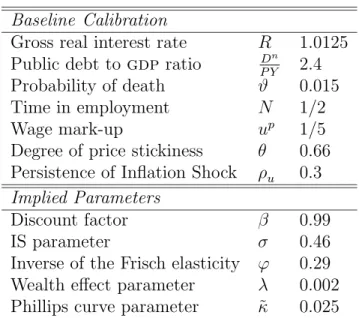
We parameterize the model assuming that each period corresponds to a quarter of year. To make the argument as transparent as possible, the model is calibrated along the lines of the existing literature. We set the steady state public debt to gdp ratio at 0.6 at annual level as in Benigno and Woodford (2003). The steady state real interest rate is 1.25%, as in McCallum (2001). The persistence of the inflation shock is set equal to ρu = 0.3. We calibrate the probability of death between two consecutive periods at ϑ = 0.015. We assume a steady state wage mark-up of up = 1/5 and set the steady
state fraction of time in employment at N = 1/2, consistently with Gal´ı, L´opez-Salido and Vall´es (2003, 2004). Finally, the probability of keeping the price fixed between two consecutive quarters is set at θ = 0.66, as in Rotemberg and Woodford (1997). Table 1 summarizes the parameterization of the model and reports the implied parameter values under the assumption that V (N ) ≡ N1+ϕ/(1 + ϕ), where ϕ = V′′
(N ) N/V′
(N ) is the inverse of the Frisch elasticity.
Figure 1 plots the responses of the economy to a positive inflation shock for different values of the monetary policy coefficient on inflation: φπ = 0.85, as in the pre-Volcker era (Taylor 1999), φπ = 1.5 (Taylor, 1993) and φπ = 0 (i.e. the case of a pure interest rate peg). A close inspection of impulse response functions reveals that even a monetary policy rule that responds to increases in inflation with a less than one-to-one increase in the nominal interest is stabilizing, contrary to the predictions of the standard New Keynesian models in which the equilibrium would be indeterminate.
inflation shock, both output and the real interest rate decline significantly. For φπ = 0.85,
as in the pre-Volker era, we observe similar dynamic responses to a positive inflation shock, though the contraction of output is larger while the real interest rate decline is less sharp. On the other hand, for an inflation coefficient of φπ = 1.5 the real interest rate and output move in opposite directions, consistently with the standard theory.
The intuition for the economic mechanism underlying these results is the following. After an inflation shock, real wealth of currently alive generations declines and output moves downwards. Inflation redistributes resources from current to future generations, since the decline in the real value of government liabilities reduces the tax load for yet unborn individuals. The presence of wealth effects in the is equation does enhance the stability of the system, making the respect of the Taylor principle unnecessary. Follow-ing a positive inflation shock, the negative effects on both output and the real interest rate come about because wealth effects tend to reduce aggregate demand redistributing resources from currently alive to future generations.
4
Conclusions
This paper has demonstrated how the explicit consideration of wealth effects in a baseline New Keynesian model can explain the decrease in output in response to an inflation shock in a way consistent with recent empirical evidence. Specifically, it has been shown that an inflation shock generates a negative effect on aggregate demand even under a passive monetary policy. An increase in inflation does not need to be counterbalanced by a more than proportional increase in the nominal interest rate to ensure economic stability.
In conclusion, our results suggest a possible simple solution to the seeming conflict between empirical evidence and the predictions of the existing New Keynesian literature regarding the effects of inflation shocks.
References
Ascari, G. and N. Rankin (2006), Perpetual Youth and Endogenous Labour Supply: A Problem and a Possible Solution. Journal of Macroeconomics, forthcoming.
Benigno, P. and M. Woodford (2003), Optimal Targeting Rules for Monetary and Fiscal Policy. NBER Macroeconomics Annual Conference, April, 4-5, 2003.
Blanchard, O. J. and C. M. Kahn (1980), The Solution of Linear Difference Models under Rational Expectations. Econometrica 48, 1305-1311.
Blanchard, O. J. (1985), Debt, Deficits, and Finite Horizons. Journal of Political Economy 93, 223-247.
Calvo, G.A. (1983), Staggered Prices in a Utility Maximizing Framework. Journal of Monetary Economics 12, 383-398.
Clarida, R., J. Gal´ı, and M. Gertler (1999), The Science of Monetary Policy: A New Keynesian Perspective. Journal of Economic Literature 37, 1661-1707.
Fair, R.C. (2002), On Modeling the Effects of Inflation Shocks. Contributions to Macroeconomics 2, art 3.
Fair, R.C. (2005), Estimates of the Effectiveness of Monetary Policy. Journal of Money, Credit and Banking 37, 645-660.
Gal´ı, J. (2003), New Perspectives on Monetary Policy, Inflation, and the Business Cycle, in M. Dewatripont, L. Hansen, and S. Turnovsky (Eds.), Advances in Economic Theory. Cambridge: Cambridge University Press, 151-197.
Gal´ı, J., D. L´opez-Salido, and J. Vall´es (2003), Understanding the Effects of Govern-ment Spending on Consumption. ECB Working Paper Series 339.
Gal´ı, J., D. L´opez-Salido, and J. Vall´es (2004), Rule-of-Thumb Consumers and the Design of Interest Rate Rules. Journal of Money, Credit, and Banking 36, 739-764.
Giordani, P. (2003), On Modeling the Effects of Inflation Shocks: Comments and Some Further Evidence. Contributions to Macroeconomics 3, art. 1.
McCallum, B.T. (2001), Monetary Policy Analysis in Models Without Money. Federal Reserve of St. Louis Review 83, 145-160.
Mon-etary Policy and Business Cycle Analysis. Journal of Money, Credit and Banking 31, 296-316.
Piergallini, A. (2006), Real Balance Effects and Monetary Policy. Economic Inquiry, forthcoming.
Rotemberg, J. and M. Woodford (1997), An Optimizing-Based Econometric Frame-work for the Evaluation of Monetary Policy, in B. Bernanke and J. Rotemberg (Eds.), NBER Macroeconomic Annual. Cambridge MA: The MIT Press, 297-346.
Schmitt-Groh´e, S. and M. Uribe (2000), Price Level Determinacy and Monetary Policy under a Balanced-Budget Requirement. Journal of Monetary Economics 45, 211-246.
Taylor, J.B. (1993), Discretion Versus Policy Rules in Practice. Carnegie-Rochester Conference Series on Public Policy 39, 195-214.
Taylor, J. B. (1999), Monetary Policy Rules. Chicago: The University of Chicago Press.
Woodford, M. (2003), Interest and Prices. Princeton and Oxford: Princeton Univer-sity Press.
Yaari, M.E. (1965), Uncertain Lifetime, Life Insurance, and the Theory of the Con-sumer. The Review of Economic Studies 32, 137-150.
Appendices
A. Derivation of Equation (13)
Using expression (11), we can write Bs,t+1(j)
Rt
= Et{Qt,t+1(s, j)Bs,t+1(j)} . (1A)
Thus, the individual flow budget constraint (4) (which at optimum holds with equality) takes the following form:
where Ys,t(j) = Ws,t(j) Ns,t(j)+Zs,t(j)−Ts,t(j). Form (2A), imposing the transversality
condition (12), we obtain the intertemporal budget constraint:
Et ∞ X T =t Qt,T(s, j) (1 − ϑ)T −tPTΩs,T(j) = Bs,t+ Et ∞ X T =t Qt,T(s, j) (1 − ϑ)T −tYs,t(j) + −Et ∞ X T =t Qt,T(s, j) (1 − ϑ)T −tPTV (Ns,T(j)) . (3A) From (10) we have Qt,T(s, j) PTΩs,T (j) ≡ βT −tPtΩs,t(j) , (4A) Et{Qt,T(s, j) PTΩs,T(j)} ≡ βT −tPtΩs,t(j) . (5A)
Substituting (5A) into (3A) yields
PtΩs,t(j) = Ψ " Bs,t(j) + Hs,t(j) − Et ∞ X T =t Qt,T(s, j) (1 − ϑ)T −tPTV (Ns,T(j)) # , (6A)
where Ψ ≡ [1 − β (1 − ϑ)]. This shows equation (13).
B. Derivation of Equation (19)
The aggregate budget constraint (15) can be re-written as follows:
Et{Qt,t+1Bt+1} = Bt+ Yt− PtΩt− PtV (Nt) . (1B)
Solving (1B) for Bt, substituting into (17) and using the definition of aggregate human
wealth, one obtains
Ψ−1 PtΩt = Et{Qt,t+1Bt+1} + PtΩt+ Et ∞ X T =t+1 Qt,T(1 − ϑ)T −tYT + (2B) −Et ∞ X T =t+1 Qt,T(1 − ϑ)T −tPTV (NT) .
Leading (2B) forward one period yields Ψ−1 Pt+1Ωt+1 = Bt+1+ Et+1 ∞ X T =t+1 Qt+1,T(1 − ϑ)T −(t+1)YT + (3B) −Et+1 ∞ X T =t+1 Qt+1,T (1 − ϑ)T −(t+1)PTV (NT) .
Multiplying both sides by Qt,t+1(1 − ϑ) and taking expectations gives
(1 − ϑ) Ψ−1 Et{Qt,t+1Pt+1Ωt+1} = (1 − ϑ) Et{Qt,t+1Bt+1} + (4B) +Et ∞ X T =t+1 Qt,T(1 − ϑ)T −tYT + −Et ∞ X T =t+1 Qt,T(1 − ϑ)T −tPTV (NT) . Solving (4B) for EtP ∞ T =t+1Qt,T(1 − ϑ)T −tYT−EtP ∞ T =t+1Qt,T(1 − ϑ)T −tPTV (NT),
sub-stituting into (2B) and rearranging, one obtains
PtΩt=
1
βEt{Qt,t+1Pt+1Ωt+1} +
ϑΨ
β (1 − ϑ)Et{Qt,t+1Bt+1} . (5B) This shows equation (19).
C. Steady State Analysis
The steady state, around the equilibrium conditions are log-linearized, is such that Yt=
Y > 0, Ω > 0, Pt= P > 0, M Ct= M C > 0, Rt= R > 1, B > 0, and Dt= D > 0 for all
t ≥ 0. This steady state is also the flexible price equilibrium, where
M C = (1 + uw) V′
(Y ) = ε − 1
ε , (1C)
From equations (19) and (27) it must be that R = 1 β + ϑΨ β (1 − ϑ) B P Ω, (3C) B R = D n. (4C)
From (3C) it should be noted that as long as private agents have finite horizons (ϑ > 0) the steady state real interest rate is affected by the steady state non-human wealth. Only in the limiting case of infinite horizons (ϑ = 0) in steady state the real interest rate is pinned down by the subjective rate of time preference, R = 1/β.
D. Proof of Proposition 1
The system (35), (38), (39) and (40) can be written in matrix form as
Et{xt+1} = Mxt+ Qet, (1D)
where the vector of endogenous variables is xt =
·
πt yt dt−1
¸′
, the vector of exogenous variables is et=
· ∆dn
t ut
¸′
, and the matrices of coefficients are
M = R −Rκ 0 1 σ (φπ + λ − R) 1 + λ + Rκσ − λ σ −1 0 1 , Q = 0 −R 0 0 1 0 .
The system (1D) is composed of two non-predetermined variables, πt and yt, and a
predetermined one, dt−1. Following Blanchard and Khan (1980), there exists a unique
stable rational expectations solution if and only if matrix M has two eigenvalues outside the unit circle and two eigenvalues inside the unit circle.
The characteristic equation of matrix M is of the form
where M0 = − det M = −
h
R (1 + λ) + Rκφπ
σ
i
. The characteristic equation (2D) satisfies the following conditions:
|M2| = trM = 2 + R + λ + Rκ σ > 3; (3D) P (−1) = −1 + M2− M1+ M0 (4D) = − · 2 (2 + λ) (1 + R) + Rκ (2 + λ + 2φ) σ ¸ < 0; P (1) = 1 + M2+ M1+ M0 (5D) = Rκλ σ > 0.
Conditions (3D)-(5D) are sufficient for equation (2D) to have one root inside the unit circle and two roots outside.9
9
Table 1: Calibration Baseline Calibration
Gross real interest rate R 1.0125 Public debt to gdp ratio P YDn 2.4 Probability of death ϑ 0.015 Time in employment N 1/2 Wage mark-up up 1/5
Degree of price stickiness θ 0.66 Persistence of Inflation Shock ρu 0.3 Implied Parameters
Discount factor β 0.99 IS parameter σ 0.46 Inverse of the Frisch elasticity ϕ 0.29 Wealth effect parameter λ 0.002 Phillips curve parameter κ˜ 0.025
0 2 4 6 8 10 −5 −4 −3 −2 −1 0 Ouput φ π=0.85 φ π=1.5 φ π=0 0 2 4 6 8 10 −0.5 0 0.5 1 1.5 Inflation Rate 0 2 4 6 8 10 −0.5 0 0.5 1 1.5 2
Nominal Interest Rate
0 2 4 6 8 10 −1.5 −1 −0.5 0 0.5 1
Real Interest Rate