Highlighting Charge Transfer Phenomena in Photo-catalytic Compounds Using Optical and X-ray Techniques

Alma Mater Studiorum – Università di Bologna

DOTTORATO DI RICERCA IN

Fisica

Ciclo XXX

Settore Concorsuale: 02/B1__________

Settore Scientifico Disciplinare: FIS/03____________

TITOLO TESI

Highlighting Charge Transfer Phenomena in Photo-catalytic

Compounds Using Optical and X-ray Techniques

Presentata da:

Giacomo Rossi

Coordinatore Dottorato

Supervisore

Prof. Silvia Arcelli

Prof. Federico Boscherini

1

SUMMARY

1.1.1 X Ray Absorption Fine Structure (XAFS) ... 12

1.1.1.1 The Origin of XAFS and the EXAFS formula... 13

1.1.1.2 Phenomenological Introduction to XANES ... 23

1.1.1.3 From XAFS Oscillations to the Local Structure (Computational Methods) .... 29

1.1.2 Resonant Inelastic X-Ray Scattering (RIXS) ... 32

1.1.3 High Resolution Fluorescence Detected X Ray Absorption Spectroscopy (HERFD XAS) 35 1.1.4 Optical Transient Absorption Spectroscopy ... 36

1.2 Materials Modeling ... 37

1.2.1 Density Functional Theory ... 38

1.2.1.1 The Hohenberg-Kohn Theorem ... 38

1.2.1.2 The Kohn-Sham Equation ... 40

1.2.2 Quasi-Newton Algorithms for Structural Relaxation ... 42

2 XAFS characterization of TiO2 Doped Systems for Photo-Catalysis ... 45

2.1 Doped and Undoped TiO2 (Potential Applications and Synthesis) ... 45

2.1.1 The Environmental Importance of TiO2 ... 45

2.1.2 V and V-N Doped Samples ... 46

2.2 Experimental Procedures and Setups ... 51

2.3 Data Analysis and Structural Modelling ... 51

2.3.1 EXAFS Processing ... 51

2.3.2 XANES Treatment ... 52

2.3.3 Structural Models and Simulations Settings ... 52

V-TiO2 Models ... 52

V-N-TiO2 Models ... 53

FDMNES Settings ... 55

2

2.3.5 Local Structure of Involved Atomic Species ... 58

2.3.5.1 Titanium ... 59

2.3.5.2 Oxygen ... 62

2.3.5.3 Vanadium ... 64

2.3.5.4 Nitrogen ... 68

2.3.6 Conclusions ... 70

3 Optical measurements on V-doped TiO2 samples ... 71

3.1 Optical Properties of Doped Samples... 71

3.2 Ultrafast Transient Absorption Spectroscopy Measurements ... 72

3.2.1 Samples ... 72

3.2.2 Experimental Setup ... 73

3.2.3 Results ... 73

3.2.3.1 330 nm Excitation ... 73

3.2.3.2 Exciting at Lower Energies ... 89

4 Element – specific charge transfer via high resolution X-ray spectroscopy ... 94

4.1 Samples ... 94

4.2 Experimental Setup... 95

4.3 Results and Data Processing ... 96

4.3.1 RIXS Characterization of the Samples ... 96

4.3.2 Results of the Differential Illumination HERFD XANES Experiment ... 99

4.3.2.1 Evaluation of the Differential Signal ... 99

4.3.2.2 Experimental Evidences ... 99

4.3.3 Data Interpretation ... 101

4.3.3.1 The Rigid Shift Analysis ... 101

4.3.3.2 Fit of the Differential Spectra... 102

4.4 Excitation Lifetime ... 106

Conclusions ... 108

4

ACKNOWLEDGEMENTS

Before discussing the results achieved during these last three years, I would like to thank all the people that I had the pleasure to work with. Among them, Professor Federico Boscherini is the person that mostly deserves my acknowledgements. He patiently followed all the steps of my PhD scholarship, teaching me how to perform research with an impact that matters. As well, I would like to thank Professor Luca Pasquini and all the PhD students in Bologna for the great support they gave me in these three years during which I learnt the fundamental value of teamwork. I would like to thank all the co-workers in Bologna not only for the precious teachings they gave me, but also and above all for the wonderful experiences we lived together. I want also to thank all the coworkers from other institutions for the fundamental help they gave me, making possible the achievement of this important milestone in my educational and professional career. I want to mention the ISM group in Rome and the group of Professor Miotello in Trento for the contribution they gave in the characterization of the systems described below. Last, but not least, I want to thank Professor Majed Chergui and his research group for sharing their knowledge on dynamic phenomena during the amazing period that I spent in Lausanne.

5

ABSTRACT

The best way to obtain significant results in science is to combine sophisticated experimental techniques and innovative samples. The aim of this thesis is to report an operative method to be used for the characterization of charge transfer phenomena in photo-active samples. This kind of analysis is extremely important for the doped TiO2 samples analyzed. These doped systems are promising photo-catalysts for hydrogen production from water splitting and pollutants degradation. Doping is an efficient method to decrease the energy needed to trigger the excitation of the photo-catalyst, otherwise possible only in the UV range. Identifying the role of dopants when the sample is excited is a mandatory step to understand the effects of dopants on the photo-catalytic properties of the systems. Both X-ray and optical techniques were used to characterize the samples and to follow those charge transfer phenomena induced by a visible excitation. Exploiting the unique characteristics of X Ray Absorption Fine Structure (XAFS) it was possible to determine the local structure of dopants inside the TiO2 matrix. With a differential illumination High Resolution Fluorescence Detected (HERFD) XAFS experiment an atomistic description of the light-induced charge transfer phenomena in V-doped TiO2 systems was obtained. The same physical process was also indirectly highlighted using optical ultrafast transient absorption spectroscopy. With this technique the inter-band transitions triggered by a visible light excitation were followed in real time. The combination of the two kinds of techniques made possible a complete description of the role of V dopants that, injecting charge carriers, lower the energy needed to trigger the photo-generation and surface trapping of charge carriers fundamental for the photo-catalytic processes.

6

REPORT OF ACTIVITIES

During my PhD scholarship I was mainly involved in projects focused on the application of sophisticated spectroscopic techniques to characterize a series of photo-active samples for energetic and environmental applications. In these three years I mainly learnt how to analyze XAFS spectra and obtain information about the local structure of single atomic species in a crystal structure. During the first year of my scholarship, I carried on the project started during my master thesis on metal phtalocyanines. The analysis of both EXAFS and XANES regions were performed using state of the art ab initio codes to simulate the near edge structure. All the results about this study were published in reference 1. The main project that I followed, however was focused on V and V-N co-doped TiO2 samples. The studies performed on these systems are the subject of my PhD thesis. To determine the local structure of the two dopants inside the TiO2 matrix two measurements sessions were performed. The first one, needed to measure the K edge absorption spectra of V and Ti cations was performed at the BM23 beamline of the ESRF in Grenoble (France). Soft X Ray measurements at N K edge, instead, were performed at the Bear beamline of the Italian synchrotron Elettra in Trieste (Italy). I analyzed all the XANES spectra collected comparing them with the theoretical ones simulated with FDMNES starting from models of the doped systems that I relaxed using Quantum ESPRESSO. The results obtained were published in references 2 and 3. After these first structural characterizations a differential illumination HERFD XANES experiment was performed in order to highlight charge transfer phenomena induced by a visible excitation of V-doped TiO2 samples. The measurements were collected using the RIXS spectrometer of the ID26 beamline at the ESRF in Grenoble (France). Analyzing the measured differential spectra, it was possible to identify a clear charge exchange between V dopants and Ti cations. These results are already published in reference 4. At the same time, together with the ISM group in Rome I performed optical transient absorption spectroscopy measurements in order to follow the time evolution of inter-band transitions in doped and undoped TiO2 samples in order to detect the effects of V doping. The results obtained are still unpublished.

During my PhD scholarship I spent six months at the EPFL (Switzerland), working in the group of Professor Majed Chergui. There, I performed ultrafast transient absorption spectroscopy measurements on Au-TiO2 systems. The results of this study are still unpublished. During this period, however I was also involved in a time resolved XAFS experiment at the micro XAS beamline of the SLS synchrotron in Villigen (Switzerland). The aim of the experiment was to follow in real time charge exchange phenomena appearing after UV irradiation in inorganic perovskites samples for photovoltaic applications. The results of this experiment are reported in reference 5.

During the PhD scholarship I attended the school organized by the Italian Synchrotron Light Society (SILS) in Grado. During the first two years I also attended the following courses at the University of Bologna:

• Fisica dei Sistemi a Molti Corpi (Physics of Many-Body Sysems)

• Dispositivi e Materiali per la Fotonica (Devices and Materials for Photonics)

I participated also to several prestigious conferences and meetings presenting posters or oral contribution. Below the complete list is reported:

7

• 24th Congress and general assembly of the International Union of Crystallography, Hyderabad (India), August 2017. (oral contribution)

• European XFEL users’ meeting and DESY photon science users’ meeting 2017, Hamburg (Germany), January 2017 (poster).

• Material.it 2016, Catania (Italiy), December 2016. (oral contribution).

• Meeting of the Italian society of Synchrotron Light, Bari (Italy), September 2016 (oral contribution).

• European XFEL users’ meeting and DESY photon science users’ meeting 2016, Hamburg (Germany), January 2016 (poster).

• 16th _{International Conference on X-ray Absorption Fine Structure, Karlsruhe (Germany),} August 2015 (poster).

8

LIST OF PUBLICATIONS

T. Baran, M. Fracchia, A. Vertova, E. Achilli, A. Naldoni, F. Malara, G. Rossi, S. Rondinini, P. Ghigna, A. Minguzzi and F. D’Acapito. "Operando and Time-Resolved X-Ray Absorption Spectroscopy for the Study of Photoelectrode Architectures." Electrochimica Acta 207 (2016): 16-21.

G. Rossi, M. Calizzi, V. Di Cintio, S. Magkos, L. Amidani, L. Pasquini, and F. Boscherini. "Local Structure of V Dopants in TiO2 Nanoparticles: X-ray Absorption Spectroscopy, Including Ab-Initio and Full Potential Simulations." The Journal of Physical Chemistry C 120.14 (2016): 7457-7466.

G. Rossi, F. d’Acapito, L. Amidani, F. Boscherini and M. Pedio. "Local environment of metal ions in phthalocyanines: K-edge X-ray absorption spectra." Physical Chemistry Chemical Physics 18.34 (2016): 23686-23694.

F. G. Santomauro, J. Grilj, L. Mewes, G. Nedelcu, S. Yakunin, T. Rossi, G. Capano, A. Al Haddad, J. Budarz, D. Kinschel, D. S. Ferreira, G. Rossi, M. Gutierrez Tovar, D. Grolimund, V. Samson, M. Nachtegaal, G. Smolentsev, M. V. Kovalenko, and M. Chergui. "Localized holes and delocalized electrons in photoexcited inorganic perovskites: Watching each atomic actor by picosecond X- ray absorption spectroscopy." Structural Dynamics 4.4 (2017): 044002.

G. Rossi, M. Calizzi, L. Amidani, A. Migliori, F. Boscherini and L. Pasquini. "Element-specific channels for the photoexcitation of V-doped TiO2 nanoparticles." Physical Review B 96.4 (2017): 045303.

Z. El Koura, G. Rossi, M. Calizzi, L. Amidani, L. Pasquini, A. Miotello and F. Boscherini. “XANES study of Vanadium and Nitrogen dopants in photocatalytic TiO2 thin films.” Physical Chemistry Chemical Physics, 2017.

9

10

INTRODUCTION

A complete description of a physical phenomenon can be obtained only with a wise combination of advanced techniques. The experimental procedure itself is fundamental for the achievement of high impact results. In this thesis a deep analysis of different doped photo-catalytic compounds is reported focusing on the experimental techniques employed. The aim was to find the right procedure to observe and describe the effects of dopants on the host structure including those induced charge transfer that are fundamental for photo-catalysis. In order to combine extremely good spatial and time resolutions both X ray and optical techniques were implied.

There are only a few techniques able to describe the local environment of low concentrated dopants in a host matrix. Among them, X-ray Absorption Fine Structure (XAFS)6 _{is one of the} most studied. Its unique characteristics like chemical selectivity are extremely important in several branches of material science. Several evolutions of this technique were developed in recent years thanks also to the improved brightness of synchrotron radiation sources. New and powerful experimental techniques like high energy resolution fluorescence detected (HERFD) XAFS7 _{are now possible. The main advantage of this technique obtained combining X ray} absorption and emission is the possibility to filter the fluorescence photons coming from the sample, selecting only those with an energy in a very narrow range. Below it will be clear that this peculiarity was extremely important for the characterization of the studied systems. The HERFD experiment described in this thesis is a further evolution designed to highlight the effects of a visible excitation on the atomic species composing the photo-catalyst. Using an exciting laser, it was possible to perform differential illumination measurements highlighting those changes induced in the local environment of dopants and host matrix cations.

X-ray techniques are surely the best candidates for an atomic description of functional materials, but in some cases, this is not the only information needed. Dealing with photo-active samples, optical measurements are also fundamental. Pump and probe experiments in this energy range are extremely powerful tools for the detection of inter-band transitions. Combining these results with those obtained in the X-ray experiments it is possible to obtain a comprehensive overview on the physical phenomena triggered by the visible excitation. The studied photo-catalysts were V and V-N co-doped TiO2 systems. TiO2 is nowadays one of the most studied photo-catalysts for water splitting and decontamination.8,9 _{TiO2 is} bio-compatible, abundant and not expensive. Those are three fundamental characteristics for large scale applications of this photo-catalyst. On the other hand, its efficiency is limited because its photo-catalytic properties can only be activated with UV radiation. The aim for the future is to find suitable solutions to increase the efficiency in the visible range. Among the various studied solutions doping is one of the most promising. It has been demonstrated that doping with transition metals and/or N is an efficient method to increase the absorption of TiO2 in the visible range and consequently its photo-catalytic efficiency.10 _{Some of the samples studied in} this thesis were already tested highlighting an enhancement of the photo-catalytic efficiency due to the dopants incorporation.

12

1

METHODS

1.1 E

T

In this section, the set of experimental techniques used to analyze several photo-active samples will be described. The aim is to give to the reader instruments to understand the final chapters were the experimental results are shown. For each technique, the exploited physical concepts and the potential applications will be highlighted.

All the described methods are part of the more general category of absorption spectroscopies. Some of them, like Resonant Inelastic X-Ray Scattering (RIXS) are innovative techniques obtained combining absorption and emission spectroscopies. The base of all absorption spectroscopy techniques is the study of variation of the absorption coefficient 𝜇 as a function of the incident photon energy. In general, when a radiation beam passes through a physical medium there is an attenuation that follows the Lambert-Beer’s law expressed in eq. 1.1, where 𝐼 indicates the beam intensity, 𝑥 the sample thickness and 𝐼0 the impinging beam intensity.

𝐼(𝑥, 𝐸) = 𝐼₀𝑒−𝜇(𝐸)𝑥 _1.1

The absorption coefficient can be defined using equation 1.2 where 𝜌_𝑖 are the element densities and 𝜎𝑖 are sum of the scattering and absorption cross sections.

𝜇 = ∑ 𝜎𝑖𝜌𝑖 𝑖

1.2

Changing the energy of the incident photons it is possible to trigger different phenomena. For example, using visible radiation it is possible to activate inter-band transitions while for higher energies in the X-Ray regime it is possible to excite the electrons from the core levels. This wide range of physical phenomena reflected in the absorption coefficient lead to the development of several different experimental techniques, each one focused on the detection of specific photo-induced dynamics or processes.

1.1.1 XRAY ABSORPTION FINE STRUCTURE (XAFS)

Among the various techniques based on X-Rays, absorption spectroscopy is one of the few that can provide information about the local environment surrounding a selected element. Chemical selectivity is fundamental for several studies, especially when doped materials are involved. For low dopant concentrations, standard techniques like X Ray diffraction (XRD) cannot provide any information about the structural changes induced by the doping process and above all, no information can be obtained about the chemical and electronic environment surrounding the dopants.

XAFS as well as the other absorption spectroscopies is based on the study of the absorption coefficient 𝜇. In the X-rays regime, the scattering cross section is several orders of magnitude lower than the absorption one. For this reason, 𝜇 can be considered directly proportional to the absorption cross section. In general, for wide energy intervals the behavior of the absorption

13

coefficient can be approximated using eq. 1.3 where 𝑍 is the atomic number of the target atom, 𝑚 its mass, 𝑑 the sample density and E the photon energy.11

𝜇(𝐸) ≈ 𝑑𝑍4 𝑚𝐸3

1.3

This trend can be considered only an approximation because of the presence of several discontinuities, the absorption edges, appearing when the photon energy becomes high enough to trigger electronic transitions from one of the core levels to the continuum. When this happens, there is a clear enhancement of the number of absorbed photons and a consequent fast rising of the absorption coefficient. In Figure 1.1 the typical shape of an absorption edge of Vanadium is shown. This feature appears when the energy needed to trigger the excitation of the K shell electrons is reached. The most interesting detail in this image, however is not the discontinuity itself, but the series of oscillations appearing in the energy range above the edge. These features of the absorption spectrum are called X Ray Absorption Fine Structure (XAFS). In the next paragraphs, it will be shown how from XAFS it is possible to obtain a significant quantity of information about the local structure and chemical environment surrounding the absorbing atom.

Figure 1.1: Typical X-ray absorption spectrum: the case of metallic V at the V K edge

1.1.1.1 THE ORIGIN OF XAFS AND THE EXAFS FORMULA

The modern interpretation of XAFS is mainly based on the physical mechanism described in the ‘70s by Stern, Sayers and Lytle.6 _{They elaborated an original model that correlated oscillations} in the region from 100 to 1000 eV above the absorption edge usually called Extended X-Ray absorption Fine Structure (EXAFS), to the local structure surrounding the absorbing atom. The oscillating features on the section of the absorption spectrum extending around the absorption edge (from 0 to 50-100 eV above the edge) were called X Ray Absorption Near Edge Structure (XANES) or Near Edge X-Ray Absorption Fine Structure (NEXAFS). Later it will be clear that the physical phenomenon behind the origin of both EXAFS and XANES is the same, but thanks to several approximations which can be made the description of the former one is simpler. For this reason, efficient methods for ab-initio simulation of XANES spectra appeared only in these last few years, thanks also to the constant improvement of computer performance power. Another very important region of the absorption spectrum is the pre-edge. Features appearing at energies below the main absorption edges are related to transitions of the core electrons to

14

unoccupied bound levels. For this reason, the pre-edge region is fundamental to understand the chemical environment around the absorber.

XAFS is nowadays a well-established technique and the physics mechanism behind it is well described in several books and articles.6,11–17 _{From a phenomenological point of view the origin} of XAFS is an interference phenomenon. In Figure 1.2 a schematic description of the mechanism mentioned above is reported. First, X-ray photons interact with the core electrons of the absorbing atom. It is good to remember that it is possible to tune the X-ray wavelength to excite the core electrons of a single atomic species. In the case shown in Figure 1.2, the energy is tuned to excite only the core electrons of the element labelled in green. If the photon energy is greater than the binding energy the core electrons can propagate as waves through the crystal structure until they reach the surrounding atoms where they are scattered. The superposition of the propagating and scattered electron wave-functions generates an interference pattern that changes the probability to excite the core electron of the absorber atom with other incoming X-ray photons. These small but visible changes are reflected in the absorption spectrum and the resulting effect is the X ray absorption fine structure.

Figure 1.2: Phenomenological origin of XAFS. a) the X ray beam excites one of the core electrons of the green atom. b) the excited photoelectron starts propagating as a wave until it reaches the atoms surrounding the absorber. c) The propagating electron wave is scattered creating an interference pattern that is extended also in the center of the absorber atom where core electrons are located. This interference proc ess gives rise to modulations of the absorption coefficient.

This phenomenological introduction is very useful to follow the steps of the more rigorous and quantitative description that will lead to the calculation of the standard EXAFS formula. Before starting, it is useful to define rigorously EXAFS. If 𝜇(𝐸) is the recorded absorption spectrum, 𝜇₀(𝐸) the spectrum that the absorber atom will produce if isolated (no surrounding atomic structure that means no oscillations) and Δ𝜇₀ the amplitude of the discontinuity jump near the absorption edge, XAFS is defined using eq. 1.4.

𝜒(𝐸) =𝜇(𝐸) − 𝜇0(𝐸) Δ𝜇₀

1.4

The first approximation needed to easily carry on the calculations is the one electron approximation. It means that only one of the electrons in the core levels interacts with the incoming photon. Before the excitation this electron is in its orbital indicated as |𝜓_𝑖⟩ characterized by a certain energy 𝐸_𝑖. When the X-ray photon with energy 𝐸_𝑝ℎ = ℏ𝜔 arrives, it

15

is absorbed by the electron that undergoes to a transition to a final state |𝜓_𝑓⟩ characterized by a final energy 𝐸𝑓= 𝐸𝑖 + ℏ𝜔. The transition rate 𝑤𝑓𝑖, directly proportional to the absorption

cross section and consequently to the absorption coefficient, can be calculated using Fermi’s golden rule expressed in eq. 1.5 where |𝑀𝑓𝑖|, the transition matrix element is the quantity

defined in equation 1.6 and 𝜌(𝐸𝑓), the density of final states. In eq. 1.6, 𝑉𝑖𝑛𝑡 represents the

interaction Hamiltonian associated to the electron-photon interaction. 𝑤_𝑓𝑖 = 2𝜋 ℏ |𝑀𝑓𝑖| 2 𝜌(𝐸_𝑓) 1.5 𝑀_𝑓𝑖 = ⟨𝜓_𝑓|𝑉_𝑖𝑛𝑡|𝜓_𝑖⟩ = ∫ 𝜓_𝑓∗_(𝒙)𝑉 𝑖𝑛𝑡(𝒙, 𝒕)𝜓𝑖(𝒙)𝑑3𝒙 1.6

It will be soon clear that the physical origin of XAFS is mainly related to the matrix element 𝑀_𝑓𝑖. To estimate the integral in eq. (1.6) it is necessary to evaluate the ground and excited electronic states |𝜓_𝑖⟩ and |𝜓_𝑓⟩ and the interaction potential 𝑉_𝑖𝑛𝑡 that, as indicated, is time dependent. The starting point of this calculation is the Hamiltonian of a single electron in the Coulomb atomic potential (eq. 1.7).

𝐻 = 𝒑2

2𝑚+ 𝑉(𝒓)

1.7

The final state |𝜓_𝑓⟩ can be evaluated finding the eigenstates of the Hamiltonian obtained perturbing 1.7 to take in account the electro-magnetic field of the X-ray photon. This can be done using the minimal coupling formalism. All the calculations are performed using a semi-classical approach considering a semi-classical description of the electro-magnetic wave acting on quantic atoms. The Hamiltonian 1.7 is modified using transformations 1.8, where 𝑨(𝒓, 𝑡) and 𝜙(𝒓, 𝑡) are respectively the vector and scalar electromagnetic potentials.

𝒑 → 𝒑 − 𝑞𝑨(𝒓, 𝑡) 𝑉(𝒓) → 𝑉 + 𝑞𝜙(𝒓, 𝑡)

1.8

The resulting Hamiltonian is shown in equation 1.9. The generic charge 𝑞 is substituted by the electron charge -𝑒.

𝐻 = 1

2𝑚(𝒑 + 𝑒𝑨(𝒓, 𝑡))

2

+ 𝑉(𝒓) − 𝑒𝜙(𝒓, 𝑡) 1.9

Since X-rays can be described as propagating waves it is possible to apply the radiation gauge (eq. 1.10)

16

𝜙 = 0 ∇ ⋅ 𝑨(𝒓, 𝑡) = 0 1.10

The first reasonable approximation is to consider a monochromatic X-Ray beam. This implies that the vector potential can be expressed in the easiest approximation as a propagating plane wave as shown in eq. 1.11

𝑨(𝒓, 𝑡) = 𝑨0𝑒𝑖(𝒌⋅𝒓−𝜔𝑡)+ 𝑐. 𝑐. 1.11

The scalar product 𝒌 ⋅ 𝒓, considering core electrons is enough small to expand in series the exponential as shown in equation 1.12

𝑒𝑖𝒌⋅𝒓_{= 1 + 𝑖𝒌 ⋅ 𝒓 −}(𝒌 ⋅ 𝒓)2

2! + ⋯ ≅ 1

1.12

This series can mostly be truncated at the first order, this is the electric dipole approximation. Sometimes also the second order term is relevant, especially in the pre-edge and XANES regions, where quadrupole contributions are not always negligible. In this approach, it can be shown that the perturbed Hamiltonian can be approximated as shown below:

𝐻 = 𝒑2

2𝑚+ 𝑉(𝒓) − 𝑒𝒓 ⋅ 𝑬(𝑡) = 𝐻0 − (𝒓 ⋅ 𝜂̂) 𝐸(𝑡)

1.13

The perturbing potential is therefore proportional to the scalar product between the position vector 𝒓 and the electric field polarization 𝜂̂. Substituting this in equation 1.5 and considering the direct proportionality between 𝑤𝑓𝑖 and 𝜇 it is possible to obtain equation 1.14 in which the

wave-functions of the N-1 non-interacting electrons are included. Since only linearly polarized X-rays are used in this work 𝜂̂ is constant.

𝜇(𝜔) ∝ |⟨Ψ_𝑓𝑁−1_𝜓

𝑓|𝜂̂ ⋅ 𝒓|𝜓𝑖Ψ𝑖𝑁−1⟩| 2

𝜌(𝐸𝑓) 1.14

The contribution of the non-interacting electrons, factorizing the starting and final wavefunctions, can be considered as a multiplicative parameter called 𝑆₀2 _{defined in equation}

1.15. The value of this factor if the other electrons are not absorbing is 1. 𝑆₀2 _{= |⟨Ψ}

𝑓𝑁−1|Ψ𝑖𝑁−1⟩| 2

≅ 1 1.15

Substituting 1.15 in 1.14 the absorption coefficient equation becomes 1.16 𝜇(𝜔) ∝ 𝑆₀2_|⟨𝜓

𝑓|𝜂̂ ⋅ 𝒓|𝜓𝑖⟩| 2

𝜌(𝐸_𝑓) 1.16

The dependence of the absorption coefficient from the energy of the incoming X-Ray photon is all described in equation 1.16. The origin of the XAFS oscillations must be related to changes in the final state |𝜓_𝑓⟩, since no oscillating part is introduced by the interaction potential.

The ground state |𝜓𝑖⟩ neglecting electron-electron interactions can be calculated as eigenstate

of the Hamiltonian 1.7, but the final state |𝜓_𝑓⟩ can be very hard to calculate. In the easiest case the core electron is excited to one of the unoccupied bound levels so, |𝜓_𝑓⟩, can be described as

17

an atomic orbital, like the ground state. These transitions obey to a series of laws called selection rules. For symmetry reasons, the matrix element and consequently the transition probability are 0 for all the transitions between bound levels that do not follow equations 1.17, where 𝑙 and 𝑚 are the electronic orbital angular momentum and its projection on the 𝑧 axis.

Δ𝑙 = ±1 Δ𝑚 = 0 1.17

When the electron transition is from one of the core levels to the continuum the final state calculation is not trivial. For high energy photo-electrons some reasonable approximations can be made leading to the standard EXAFS formula. The first step to simplify calculations, is to redefine all the quantities in the previous formulas as functions of the electron wave-vector 𝒌 the modulus of which is defined in a free electron approximation, in equation 1.18, where 𝑚𝑒 is

the electron mass, 𝐸₀, the absolute value of its binding energy and 𝐸 the incident photon energy.

𝑘 = √2𝑚𝑒

ℏ (𝐸 − 𝐸0)

1.18

The final state for the excited core electrons, if the photon energy is enough to promote the transition to the continuum is an outgoing wave with energy 𝐸_𝑓= 𝐸 + 𝐸_𝑖. In case of a non-isolated atom, a small perturbative contribution due to scattered photoelectrons must be added to the propagating wave. The absorption coefficient can always be evaluated using 1.16, but in this last case the final state |𝜓𝑓⟩ is defined as shown in equation 1.19 where |𝜓𝑓0⟩ is the

unperturbed final state of an isolated atom and Δ the small perturbation due to the backscattered electrons.

|𝜓_𝑓⟩ = (1 + Δ) |𝜓_𝑓0_{⟩ 1.19}

Substituting equation 1.19 in the XAFS definition (equation 1.4) and neglecting all the terms containing Δ2 _{it is possibl0e to write the explicit form of the XAFS equation (eq. 1.20)}

𝜒(𝑘) =𝜇(𝑘) − 𝜇0(𝑘)

𝜇0(𝑘) = 2 Re {Δ}

1.20

A way to calculate Δ and consequently 𝜒(𝑘) is based on the muffin-tin approximation. This kind of approximation is quite good if the photo-electron propagating outside the atom has enough energy to not be affected by the non-spherical shape of the real atomic potential. This happens only in the EXAFS region, so for the interpretation of XANES in many cases this model is not accurate enough and it is necessary to use the full atomic potential that however is more complex and computationally demanding. The muffin tin model, assumes a low range Coulomb potential centered in the various atomic sites surrounded by an inter-atomic region where the potential is constant (null for easier calculations). In Figure 1.3 a cartoon picture of such a potential is shown. With the roman numbers I, II and III are indicated three main regions that will be very useful for the evaluation of the final state |𝜓_𝑓⟩ in a single scattering approximation. The simple derivation illustrated in the following lines has the aim of showing the physical origin of the oscillating behavior of 𝜒(𝑘). The |𝜓_𝑓0_{⟩ wavefunction in region I can be very complex,}

18

but since the absorption coefficient is related to the matrix element between the final state and the localized core level only the behavior at r around 0 is relevant. Because of the selection rules the final state will have an angular momentum 𝑙 = 1 if the starting core level is the 1s. The radial part of this p orbital can be described using the spherical Bessel function 𝑗1 shown in equation

1.21 𝑗1(𝑘𝑟) = sin(𝑘𝑟) 𝑘𝑟 − cos(𝑘𝑟) (𝑘𝑟)2 1.21

The behavior of 𝑗₁ near the origin can be approximated with 𝑘𝑟/3 that is the limit for small 𝑟 values of 1.21.

Figure 1.3: Schematic description of the Muffin thin potential. The Coulomb Potential is limited in the two spherical regions I and III, while in region II is null.

In region II the radial part of the wavefunction will be described as the superposition of an incoming and an outgoing wave as shown in equation 1.31

𝜓𝐼𝐼(𝑟) =

1 𝑘𝑟[𝑒

−𝑖(𝑘𝑟−𝜋_{2)+ Φ}′_𝑒𝑖(𝑘𝑟−𝜋_2)] 1.22

The term Φ′ _{must match 𝜓}

𝐼(𝑟) and 𝜓𝐼𝐼(𝑟), because no discontinuity can appear at the interface

between region I and II. Since in the transition between region I and II the probability to find the propagating electron must be conserved the coefficient Φ′ must have a unit modulus. This means that this parameter act as a dephasing coefficient. Without scattering atoms surrounding the absorber equation 1.31 is simplified to a propagating wave. Considering also the angular dependence, the representation in spherical coordinates of the unperturbed wavefunction |𝜓_𝑓0⟩ can be written as

19 ⟨𝑟, 𝜃, 𝜙|𝜓_𝑓0_{⟩ = 𝜓} 𝐼𝐼0(𝒓) =√3_4𝜋cos𝜃 1 𝑘𝑟Φ𝑒𝑖𝑘𝑟 1.23 where Φ is equal to −𝑖Φ′.

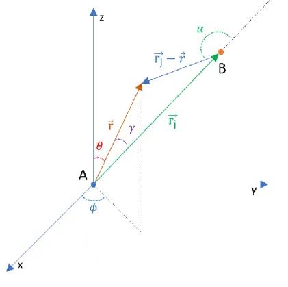
The scattered wavefunction generating the incoming wave in equation 1.22 can be derived using a standard formalism with the reasonable assumption of a point like scattering atom. Defining 𝒓𝑗 as the interatomic vector, 𝜓𝑠𝑐(𝒓) can be written as:

𝜓_𝑠𝑐(𝒓) = 𝜓𝐼𝐼(𝒓)𝑓(𝑘, 𝑟𝑗, 𝛼)

𝑒𝑖𝑘|𝒓−𝒓𝒋| 𝑘|𝒓 − 𝒓_𝒋|

1.24

where 𝑓(𝑘, 𝑟𝑗, 𝛼) is the scattering amplitude depending on the momentum 𝑘, the distance 𝑟𝑗 and

the scattering angle 𝛼. To better understand the situation in Figure 1.4 a simple sketch is shown.

Figure 1.4: Schematic description of the single scattering phenomenon. A and B are respectively the Absorber and the scattering atom

The last multiplicative term in the r.h.s of equation 1.24 is the typical expression of a spherical wave centered in B. Since only the part of the scattered wave with the same angular dependence and the same limit for 𝑟 → 0 as the unperturbed wavefunction |𝜓_𝑓0⟩ will gives rise to relevant contributions generating the fine structure, the strategy is to calculate a factor C such that:

20 lim 𝑟→0𝜓𝑠𝑐(𝒓) = 𝐶√3 4𝜋 cos 𝜃 𝑘𝑟 3 Φ 1.25

For small 𝒓 values the quantity |𝒓 − 𝒓_𝒋| can be approximated as shown in equation 1.26

|𝒓 − 𝒓𝒋| ≈ 𝑟𝑗− 𝑟 cos 𝛾 1.26

The spherical wave term for small 𝑟 and 𝑘𝑟𝑗 ≫ 1 becomes:

𝑒𝑖𝑘|𝒓−𝒓𝒋| 𝑘|𝒓 − 𝒓_𝒋|≈ 𝑒𝑖𝑘𝑟𝑗 𝑘𝑟_𝑗 [1 + ( 1 𝑘𝑟_𝑗− 𝑖) 𝑘𝑟 cos 𝛾] ≈ 𝑒𝑖𝑘𝑟𝑗 𝑘𝑟_𝑗 [1 − 𝑖𝑘𝑟 cos 𝛾] 1.27

Writing cos 𝛾 as a function of 𝜃 and 𝜃𝑗 it is possible to identify the portion of scattered

wavefunction having the behavior described in equation 1.25. The value of the C factor obtained at the end of the calculation is reported in equation 1.28.

𝐶(𝑘, 𝑟_𝑗, 𝜃_𝑗) = −3𝑖𝑒2𝑖𝑘𝑟𝑗 𝑘2_𝑟 𝑗2 cos2_𝜃 𝑗𝑓(𝑘, 𝑟𝑗, 𝜋) 1.28

To take in account the effects of the absorbers’ potential on the scattered wave, C must be multiplied by a phase shift term 𝑒2𝑖𝛿1. For small 𝑟 values (where the starting core levels are localized) the final wavefunction obtained adding the outgoing unperturbed wavefunction and the incoming scattered wave is described in equation 1.29 from which it is possible to derive the value of the Δ factor defined in equation 1.19.

|𝜓_𝑓⟩ = (1 + 𝐶𝑒2𝑖𝛿1)|𝜓

𝑓0⟩ = (1 + Δ)|𝜓𝑓0⟩ 1.29

The fine structure 𝜒(𝑘) can be easily derived substituting the value of Δ in equation 1.20 obtaining: 𝜒(𝑘) = 2 Re {Δ} = 3 cos2_𝜃 𝑗Im { 𝑒2𝑖𝑘𝑟𝑗 𝑘2_𝑟 𝑗2 𝑓(𝑘, 𝑟𝑗, 𝜋)𝑒𝑖2𝛿1} 1.30

Approximating the wave impinging on the scattering atom as a plane wave it is possible to remove the dependence of the scattering amplitude from 𝑟_𝑗 and express 𝑓 as shown in equation 1.31.

𝑓 = |𝑓(𝑘, 𝜋)|𝑒𝑖𝜙 _1.31

With approximation 1.31 it is possible to write the standard EXAFS formula (equation 1.32) 𝜒(𝑘) = 3 cos2𝜃𝑗

𝑘2_𝑟2 |𝑓(𝑘, 𝜋)| sin[2𝑘𝑟𝑗+ 𝜙 + 2𝛿1]

1.32

For randomly oriented powder samples or amorphous materials the average value of 3 cos2_𝜃 𝑗

21

The generalization of equation 1.38 to the case of several nearest neighbors is immediate and it is given by the summation of all the contributions coming from the atoms at distance 𝑅_𝑖 obtaining equation 1.33, where 𝑁_𝑖 indicates the degeneracy of the 𝑖𝑡ℎ _{single scattering path. The}

dephasing contributions are resumed for simplicity in the 𝜙_𝑖(𝑘) terms. 𝜒(𝑘) = ∑ 3𝑁_𝑖(𝜂̂ ⋅ 𝑹_𝒊)2 1

𝑘𝑅_𝑖2|𝑓(𝑘, 𝜋)| sin(2𝑘𝑅𝑖 + 𝜙𝑖(𝑘)) 𝑖

1.33

This formula, however needs some changes to take in account several important physical effects like disorder, multiple scattering and inelastic processes.

Inelastic processes introduce two multiplicative factors. The first one, 𝑆₀2_{, was previously}

defined as the contribution of the non- interacting electrons while the second one is a decreasing exponential factor 𝑒−𝑅𝑖𝜆 related to the mean free path of the photoelectron. Without inelastic scattering processes the mean free path is the distance that the photo-electron can travel before the core-hole excitation decays as shown in equation 1.34 where 𝑣 is the photo-electron velocity and 𝜏𝑢 the core-hole life-time

𝜆_𝑢 = 𝑣 ⋅ 𝜏_𝑢 1.34

However, the mean free path is limited also by the energy losses due to inelastic scattering processes. The mean free path in this case, indicated as 𝜆_𝑒, is quite difficult to quantify. Since both contributions (core-hole and inelastic dumping) are relevant it is necessary to define a parameter 𝜆 (a function of 𝜆_𝑒and 𝜆_𝑢) describing the actual value of the mean free path (equation 1.35). 1 𝜆 = 1 𝜆_𝑢+ 1 𝜆_𝑒 1.35

It is easy to understand that longer scattering paths are thus less probable and, consequently they give a lower contribution to the EXAFS signal. Considering inelastic contributions the standard EXAFS equation is 1.36

𝜒(𝑘) = 𝑆₀2_{∑ 3𝑁} 𝑖(𝜂̂ ⋅ 𝑹𝒊)2 1 𝑘𝑅_𝑖2𝑒− 2𝑅𝑗 𝜆 |𝑓(𝑘, 𝜋)| sin(2𝑘𝑅_𝑖+ 𝜙_𝑖(𝑘)) 𝑖 1.36

As mentioned before, not only single scattering contributions are relevant to correctly reproduce the EXAFS signal. The photo-electron can be scattered by several atoms before coming back to the absorber center. The absorption coefficient can be expressed as the sum of a series of contributions as shown in equation 1.37, where the subscripts indicate the number of scattering processes that the photo-electron undergoes before going back to the absorber.

𝜇(𝑘) = 𝜇0(1 + 𝜒1(𝑘) + 𝜒2(𝑘) + 𝜒3(𝑘) + ⋯ ) 1.37

In the EXAFS region, this series is strongly converging (this is not true for XANES region), so it is possible to reproduce quite well the experimental signal considering only the first two or three 𝜒_𝑖terms, neglecting all the paths involving a higher number of scattering processes. Each

22

𝜒_𝑖 function can be expressed as shown in equation 1.38, where {𝒓_𝑖} are the partial distances composing the multiple scattering path and 𝑅_𝑖 the total path length. 𝐴 and 𝜙 depend on the potentials of the atoms involved in the multiple scattering process.

𝜒_𝑖(𝑘) = 𝐴𝑖(𝑘, 𝒓𝑖) sin(𝑘𝑅𝑖 + 𝜙𝑖(𝑘, 𝒓𝑖)) 1.38

As mentioned before, it is necessary to take in account also the contributions related to the structural disorder. Oscillations of the atoms around their equilibrium positions, can modify the interference phenomenon generating EXAFS. Small oscillations of the crystal structure, slightly distorting the local structure, can lower the effects of constructive or destructive interferences. The result is a smoother XAFS spectrum with lower features. In the standard EXAFS formula, the disorder contribution is represented by the so-called Debye Waller factors 𝜎_𝑖2 _{that represent the mean square fluctuation of the scattering path lengths. The decreasing}

exponential term 𝑒−𝑘2_𝜎

𝑖2 strongly damps EXAFS oscillations when 𝜎_𝑖 or 𝑘 are too high and since 𝜎_𝑖2 _{increases with the temperature, it is sometimes needed to cool down the sample to have an}

acceptable signal. The final form of the standard EXAFS formula can be expressed as shown in equation 1.39. 𝜒(𝑘) = 𝑆₀2_{∑ 3𝑁} 𝑖(𝜂̂ ⋅ 𝑹𝒊)2 1 𝑘𝑅_𝑖2𝑒−( 2𝑅𝑖 𝜆 +2𝑘2𝜎𝑖2) _{|𝑓(𝑘, 𝛼} 𝑖)| sin(2𝑘𝑅𝑖+ 𝜙𝑖(𝑘)) 𝑖 1.39

Since the EXAFS signal can be expressed as the sum of sinusoidal functions depending by the path half-lengths 𝑅_𝑖, its Fourier transform in the radial distances space is a series of peaks centered in values related to the inter-atomic distances. An example is shown in Figure 1.5 where Fourier transforms of V and V2O4 are compared. Without performing a complete analysis with ab initio codes, starting from equation 1.39 it is possible to extrapolate some information. For example, it is immediately visible that V-V bonds in the V foil are longer than the V-O bonds in V2O4. This because the most intense peak at low R values, related to the first correlation shell less affected by inelastic effects, is centered at a lower position for the oxide. This is of course confirmed by crystallographic data18 _{that shows a V-V distance of around 2.62 Å wider than the} average V-O distance in V2O4 that is around 1.90 Å.

Figure 1.5: Comparison between the Fourier transform of the 𝜒(𝑘) signals of V (black curve) and V2O4 (red curve)

23

1.1.1.2 PHENOMENOLOGICAL INTRODUCTION TO XANES

The aim of this paragraph is to show how XANES spectra can provide crucial information about the studied systems also without any theoretical calculation. Some of the spectral features appearing near the absorption edge are strictly related to the chemical environment surrounding the absorber. Later in this work edge shifts and changes in the pre-edge features will play a key role in data interpretation, so a brief description of the physics behind these phenomena is required to fully understand the results obtained.

THE PRE-EDGE

In Paragraph 1.1.1.1 above, discussing the origin of XAFS, pre-edge features were related to dipole and quadrupole transitions from core levels to unoccupied bound states. These peaks are of great importance in the study of transition metals oxides because of their extreme sensitivity to local structure and symmetry changes. In Figure 1.6 the pre-edge features of TiO2 anatase and rutile and FeTiO3 ilmenite are shown. In all the three cases Ti is in a 4+ oxidation state and the surrounding oxygens are placed in the vertexes of distorted octahedrons. The three local structures are very similar, but bond lengths and angles are enough different to produce significant changes in the pre-edge structure.

When the local symmetry changes more significantly, the effects on pre-edge can be even more dramatic. For example an interesting study performed by Wong et al.19 _{on Vanadium oxides} highlights the correlation between the presence of an inversion center and the amplitude of the edge peaks. This kind of correlation between local symmetry and amplitudes of the pre-edge features is valid also for the other transition metals as shown in reference 20_.

Figure 1.6: Comparison between the pre-edges of TiO2 (Anatase and Rutile) and FeTiO3 (ilmenite)

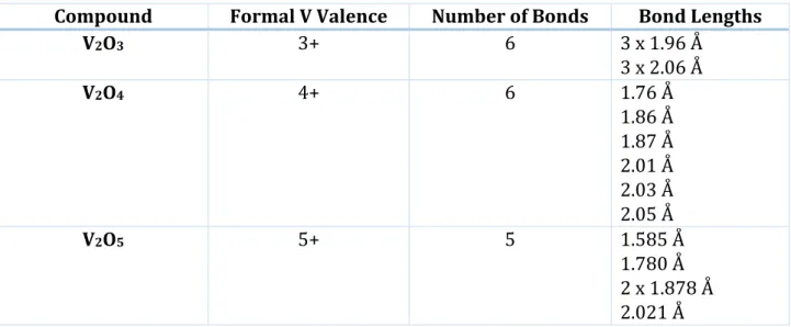
Considering the three most abundant V oxides (V2O3, V2O4 and V2O5) it is possible to see that the local structure surrounding V changes significantly, increasing the V oxidation state. In V2O3, V3+ _{cations are in the center of slightly distorted oxygen octahedrons. This structure showing} only two possible lengths for the six V-O bonds is still a quite regular octahedron. In V2O4, V4+ cations are surrounded by even more distorted oxygen octahedrons showing six different V-O

24

bond lengths. The local structure of V2O5, instead, is completely different. V5+ _{cations are placed} at the center of a distorted square based oxygen pyramid. In Table 1.1 are listed some relevant structural parameters of these three compounds obtained from the literature19_.

Table 1.1: Relevant structural parameters for three of the main abundant V oxides. Values are obtained from reference 19

Compound Formal V Valence Number of Bonds Bond Lengths

V2O3 3+ 6 3 x 1.96 Å 3 x 2.06 Å V2O4 4+ 6 1.76 Å 1.86 Å 1.87 Å 2.01 Å 2.03 Å 2.05 Å V2O5 5+ 5 1.585 Å 1.780 Å 2 x 1.878 Å 2.021 Å

In Figure 1.7 the comparison of pre-edge peak intensity for the three compounds is shown. The less symmetric V2O5 shows the highest peak, while V2O3 pre-edge feature is almost negligible. This phenomenon can be explained on the basis of group theory.21 _{The key concept is that, for} non-centrosymmetric structures like V2O5 the hybridization of d and p orbitals is possible and consequently the pre-edge peaks are intense because of the allowed dipole transition from core 1s to p levels. This kind of hybridization is impossible in regular octahedral structures with an inversion center. This explains why V2O3 shows the weaker pre-edge feature in Figure 1.7.

Figure 1.7: Pre-edge peaks of three V oxides.

This behavior is rather general among transition metal oxides as reported in several studies on other compounds.20,22

25

The edge is defined as the onset of the continuum state and its position (E0) is strictly related to the oxidation state of the absorber. This dependence can be easily explained using a simplified model as shown in Figure 1.8.

The strongest force acting on core electrons is the Coulomb interaction with the positive nucleus. The presence of other electrons, however generates a not-negligible repulsive electric field that lowers the energy needed to extract the electron from the atomic potential. This electron-electron contribution generates a screening of the Coulomb interaction between electrons and nucleus and for this reason is known as screening potential. The oxidation state of an atom depends on its electronic configuration when incorporated in a molecule. Some of the valence electrons can be transferred from or to the ligand species, depending on their electro-negativity. This change of electronic configuration influences the screening potential of the absorber atom. If the oxidation state rises (the atom donates charges to the ligands) the screening decreases and a higher energy is necessary to promote the electron transition to the continuum. On the other hand, in case of oxidation state reduction the electron transition to the continuum is favored and the needed energy is lower.

This correlation between edge position and oxidation state is very useful for XANES data interpretation. Comparing the edge position of an unknown sample with some references it is possible to have an indication of the oxidation state of the absorber in the unknown compound. The edge position E0 can be easily evaluated finding the maximum of the spectrum derivative after the pre-edge region. Also in this case V oxides are very useful for a graphic and immediate representation of the physical concept. In Figure 1.9 it is shown how the edge position shifts to higher energies increasing V oxidation number. It is important to notice that a change of 1 in oxidation state can produce a visible shift of the edge of a few eV.

26

Figure 1.8: schematic description of the edge shift phenomenon. The interaction between the elements Z and Z2 produces a lowering of the repulsive screening potential and a consequent increasing of E0. In the right schemes Ez stays for the not-screened Coulomb potential while Escreen is the potential contribution due to electron-electron repulsion. The atomic potential is schematically simplified as a parabolic potential centered in r0 that represent the average value of the distance between the electron and the nucleus.

27

Figure 1.9: Comparison of the Edge position for V2O3 (V3+), V2O4 (V4+) and V2O5 (V5+). The edge position is clearly a function of the oxidation state.

POST EDGE REGION

The post-edge region is the section of the XANES spectrum generated by the interference of outgoing and scattered photo-electron wave-functions, the same physical mechanism discussed for EXAFS in paragraph 1.1.1.1. We mentioned above that the oscillating signal for EXAFS in a muffin-tin approach can be reconstructed using only a few scattering processes. In the XANES region, however, using the same approach it is possible to demonstrate that the series in equation 1.37 does not converge, so to obtain a satisfactory description of the near edge region is mandatory to consider all the possible multiple scattering paths. This approach is called full multiple scattering. Several codes for ab initio calculations rely on this kind of approach.14,23 _{Recently, new methods were developed to overcome the muffin tin}

28

approximation and the full multiple scattering approach. In this work FDMNES,24 _{will be mainly} used, but several other codes based on DFT calculations are in continuous development.25 _A brief description of FDMNES will be given in paragraph 1.1.1.3.

THE LINEAR COMBINATION ANALYSIS

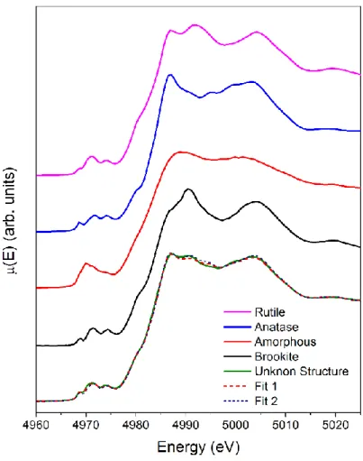
A common method to perform analysis of the XANES spectra of mixtures or multiphase compounds is the linear combination analysis. Starting from the spectra of selected reference species is sometimes possible with a linear combination fitting to reconstruct the unknown spectrum. In Figure 1.10 the application of this method to one of the V-TiO2 nanoparticle samples studied in this work is shown. From XRD it is known that the overall structure of this nanoparticles is a superposition of three TiO2 polymorphs (Rutile Anatase and Brookite). The advantage of using XANES instead of XRD, however is the possibility to use as reference spectra also those generated by low range ordered structures (amorphous) that are not detectable with XRD. In Figure 1.10 are shown two fits obtained with or without the spectrum of an amorphous TiO2 sample (red solid curve). Using the linear combination fitting routine of the software Athena26 _{it is possible to obtain the relative percentages of the different polymorphs and the 𝜒}2 merit function as shown in Table 1.2.

29

Table 1.2: Percentages of the standards used to fit the unknown structure. The fit including the amorphous structure gives a better value of 𝜒2 _{and a major agreement with the unknown spectrum.}

Fit Rutile Percentage Anatase Percentage Brookite Percentage Amorphous Percentage 𝝌𝟐 Fit 1 28% (4%) 44% (1%) 12% (2%) 15% (2%) 0.009 Fit 2 41% (4%) 43% (4%) 16% (3%) - 0.019

1.1.1.3 FROM XAFSOSCILLATIONS TO THE LOCAL STRUCTURE (COMPUTATIONAL METHODS)

The phenomenological approach to XAFS described in the previous chapter can be followed by a more rigorous description based on ab initio calculations. The XANES lineshape can be interpreted to understand which structural model gives rise to the specific interference pattern behind XAFS spectra. The approaches for EXAFS and XANES used in all the characterizations described in this work are slightly different. For both methods, a starting set of coordinates is needed. This set can be obtained from X Ray Diffraction (XRD) patterns in case of standard compounds or calculated ab initio with specific codes in case of engineered materials. Further in chapter 1.2 the theoretical background behind the density functional theory calculation of these coordinate sets will be briefly described.

The standard procedure for EXAFS is to fit the experimental signal with a theoretical one generated using the guessed structure. The fit procedure implemented in the IFEFFIT27 _code refines some of the parameters in the EXAFS formula (equation 1.39) . The best model is obviously the one better describing the experimental signal, but a good agreement is not sufficient. The goodness of a theoretical model depends also from the values of the refined parameters that must be reasonable.

For XANES, as mentioned in section 1.1.1.1 the muffin tin potential is not always a good approximation. Several full potential approaches were developed in these last years.24,25 _These kind of calculations, however can be very time demanding, so a real fit is very difficult. Simulating several spectra slightly varying the starting structural configurations could take months with a normal calculator, so the approach adopted during my PhD was to choose between the various theoretical models the one that generates a theoretical XANES spectrum comparable with the experimental data. This means that XANES analysis are less quantitative than EXAFS ones, but the number of free parameter used is a lot less.

In the following paragraphs, the two codes used for EXAFS and XAFS analysis will be briefly described. The first one, FEFF14_{, is a world-wide known software for the analysis of the} extended region. The other software is FDMNES,24,28 _{one of the most recent software for full} potential ab initio calculation of the XANES region.

FEFF

FEFF14 _{and IFEFFIT}27 _{are two packages developed by researchers from the Seattle group to} analyze EXAFS spectra. They can be used from the command line or with the graphical user interface Demeter26 _{that contains also several useful tools for data treatment.}

30

As demonstrated in section 1.1.1.1 the EXAFS signal can be reproduced as the sum of several contributions related to different scattering paths according to eq. 1.40 where the index 𝑖 is related to a single or multiple scattering path.

𝜒(𝑘) = ∑ 𝜒𝑖(𝑘) 𝑖

1.40

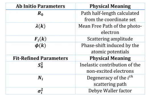
FEFF, starting from a user-defined set of atomic coordinates, calculates all the possible scattering paths and their contributions to the overall EXAFS signal using equation 1.41, where 𝑘 and 𝑅_𝑖 are calculated from equation 1.42 and 1.43.

𝜒𝑖(𝑘) = 𝑁_𝑖𝑆₀2_𝐹 𝑖(𝑘) 𝑘𝑅_𝑖2 sin(2𝑘𝑅𝑖 + 𝜙(𝑘))𝑒−2𝑘 2_𝜎 𝑖2𝑒− 2𝑅𝑖 𝜆(𝑘) 1.41 𝑅_𝑖 = 𝑅₀+ Δ𝑅_𝑖 1.42 𝑘2 ₌2𝑚(𝐸 − 𝐸0) ℏ2 1.43

The number of parameters in these equations is big, so the meaning of each symbol is explained in Table 1.3. Some of these parameters are calculated by FEFF starting from the cluster potential modeled with the muffin tin approximation. Not all the parameters can be calculated

ab initio. Some of them like the Debye Waller factors (related to the sample temperature and

intrinsic disorder) must be refined by IFEFFIT during the fit procedure starting from reasonable guessed values. In Table 1.3 are listed all the parameters divided in the calculated and fit refined categories.

Table 1.3: Description of the parameters needed to produce the theoretical signal Ab Initio Parameters Physical Meaning

𝑹_𝟎 Path half-length calculated from the coordinate set 𝝀(𝒌) Mean Free Path of the

photo-electron

𝑭_𝒊(𝒌) Scattering amplitude

𝝓(𝒌) Phase-shift induced by the atomic potentials

Fit-Refined Parameters Physical Meaning

𝑺_𝟎𝟐 _{Inelastic contribution of the}

non-excited electrons

𝑵_𝒊 Degeneracy of the 𝑖𝑡ℎ

scattering path

31

𝚫𝑹 Variation of the path half-length

𝑬_𝟎 Energy Shift

IFEFFIT can perform fits in the 𝑘 or R space modelling the theoretical signal to reproduce 𝜒(𝑘) or its the Fourier transform 𝜒(𝑅). This last is sometimes preferred, providing direct information about the interatomic distances of the first atomic shells.

The goodness of a fit, both in k or in R space, can be evaluated with a merit function r defined, as shown in equation 1.44. Lower is the value of the merit function and better is the agreement between experimental data and calculated signal.

r =∑[𝜒𝑜𝑏𝑠𝑒𝑟𝑣𝑒𝑑 − 𝜒𝑓𝑖𝑡]

2

∑[𝜒_{𝑜𝑏𝑠𝑒𝑟𝑣𝑒𝑑}]2

1.44

As previously mentioned minimization of r is not sufficient to have a good fit. The values of fit parameters should be physically reasonable. When the number of parameters used is too high the fit can give misleading results due to unwanted correlations between the various parameters. A way to handle this problem and perform a meaningful fit is to relate with mathematical constrains several parameters reducing the number of free ones. In one of the papers published during my Phd course1 _{based on EXAFS and XANES analysis of} phthalocyanine compounds, adopting some results from Haskel29 _{and Poiarkova,}30 _{a significant} reduction of the parameters number was possible relating some of the multiple scattering Debye Waller Factors to those of single scattering paths.

FDMNES

The calculation of the theoretical XANES spectrum is way more complex than the EXAFS one. The muffin tin approximation and the related multiple scattering approach, can be sometimes inadequate as shown by Kravstova and co-workers.31 _{They compared the theoretical spectra} calculated using a muffin tin based software (FEFF14_{) and a full potential one (FDMNES}24_{). The} full potential approach is shown to well reproduce all the anatase features, better than the multiple scattering code. Since the samples analyzed in this work are mostly based on TiO2 polymorphs, FDMNES seemed to be the best candidate to reproduce their absorption spectra. In this paragraph, a brief description of FDMNES will be shown. Detailed descriptions of the code can be found in references.24,28,32 _{Since FDMNES is a full potential software, parts of its} code are based on simplified versions of the Density Functional Theory described in Chapter 1.2.1. The first step, is a self-consistent calculation to get the starting charge configuration and electronic potential surrounding the absorber. The Coulomb potential of the atomic cluster surrounding the absorber is evaluated solving the Poisson equation once the charge density is evaluated with the LDA -U technique. To calculate XANES spectrum, it is necessary to assume an excited electronic configuration for the absorber. This is implemented placing the core electron in the first available unoccupied level. The core of the calculation is the evaluation of the final state |𝜓_𝑓⟩ in equation 1.16. This is performed solving the Schrodinger equation with the finite difference method. This approach consists in constructing a space grid and discretizing the Schrodinger equation on its points. Of course, the Coulomb potential in the

32

Schrodinger equation is the one obtained previously with the iterative self-consistent calculation. This means that no approximation is made on the shape of the potential, overcoming the muffin tin approximation. The final state wave-function is then used to calculate the matrix element 𝑀𝑓𝑖 and consequently the absorption spectrum.

The theoretical absorption spectrum requires often to be convoluted before the comparison with the experimental data, because of the broadening due to the core-hole width Γ_{ℎ𝑜𝑙𝑒} and to the spectral width 𝛾(𝜔) of the final state. This convolution is made using an energy dependent Lorentzian function Γ𝑓.

1.1.2 RESONANT INELASTIC X-RAY SCATTERING (RIXS)

Until now, only X ray absorption techniques were described, however combining them with X-ray emission spectroscopy (XES) it is possible to obtain an extremely powerful technique called Resonant Inelastic Scattering (RIXS) giving a wider range of information about the chemical properties of the absorbers’ environment. XES can be classified in two regions. If the incoming photon energy (indicated with ℏΩ) matches one of the absorption edges of the selected element the result is a resonant mechanism of excitation and emission passing through a core-hole excited state. The emission spectrum in this case is strongly dependent from the incident photon energy ℏΩ. This is the base phenomenon exploited in the so-called resonant X-ray Emission spectroscopy (RXES). If the incoming photon energy is well above the absorption edge the dependence from Ω vanishes and the emission phenomenon is labelled as normal. For this the relative technique is also called normal X-ray emission spectroscopy (NXES).

It is easy to understand that RXES is a lot more interesting than NXES. Depending on the emitted photon energy (ℏ𝜔) RXES can be divided in two sub-categories. If 𝜔 is equal to Ω the phenomenon is called resonant elastic X ray scattering (REXS), while if 𝜔 is lower than the incoming photon energy, the sample absorbs part of the photon energy and the process is called inelastic X-ray scattering (RIXS). RIXS is a very powerful tool to study the electronic states in solids and in the next paragraphs the theory behind this experimental technique will be briefly described. There are already several reviews about this topic, and the formalism used in this section is the same used in references 7,33_.

The interaction between electrons and photons was previously described in section 1.1.1.1 with a semiclassical approach. The perturbative potential can be written as:

𝐻_𝐼𝑛𝑡 = 𝑒 𝑚_𝑒𝑐∑ 2𝒑𝑗⋅ 𝑨(𝒓𝑗) 𝑗 + 𝑒2 2𝑚_𝑒𝑐2∑ 𝑨(𝒓𝑗) 2 𝑗 1.45

The incoming photons as previously mentioned have an energy ℏΩ and its wave-vector is labelled as 𝒌₁. On the other hand, the emitted photon energy, is indicated with ℏ𝜔 and its wave-vector as 𝒌₂. The differential scattering cross section can be derived in the minimal coupling formalism using the Kramers-Heisenberg equation (equation 1.46) where Ω_𝒌2 is the solid angle of collection and 𝑊12 is the transition rate.

𝑑2_𝜎 𝑑Ω_𝒌2𝑑𝜔= 𝜔2 𝑐4 ( 1 2𝜋) 3 𝑊₁₂ 1.46

33

𝑊₁₂ can be calculated according to Fermi’s golden rule, however it is necessary to remind that this kind of process is composed by two different steps (absorption and emission). Indicating with |𝑔⟩, |𝑖⟩, |𝑗⟩ respectively the unexcited state, the core-hole intermediate state and the final state after the emission, the rate 𝑊12 can be calculated as shown in equation 1.47.

𝑊₁₂= ∑(2𝜋)3 Ω𝜔 ( 𝑒2 𝑚_𝑒) 2 𝛿(𝐸_𝑗− 𝐸_𝑔+ 𝜔 − Ω) 𝑗 × |[⟨𝑗|𝝆𝒌1−𝒌2|𝑔⟩(𝜼1⋅ 𝜼2) + 1 𝑚∑ ( ⟨𝑗|𝒑(𝒌2) ⋅ 𝜼2|𝑖⟩⟨𝑖|𝒑(−𝒌1) ⋅ 𝜼1|𝑔⟩ 𝐸_𝑖− 𝐸_𝑔 − Ω 𝑖 +⟨𝑗|𝒑(𝒌1) ⋅ 𝜼1|𝑖⟩⟨𝑖|𝒑(−𝒌2) ⋅ 𝜼2|𝑔⟩ 𝐸_𝑖 − 𝐸_𝑔 − ω )]| 2 1.47

The quantities 𝒑(𝒌) and 𝝆(𝒌) are defined as

𝒑(𝒌) = ∑ 𝒑𝑛𝑒−𝑖𝒌⋅𝒓𝑛 𝑛

𝝆(𝒌) = ∑ 𝑒−𝑖𝒌⋅𝒓𝑛

𝑛

1.48

where the index 𝑛 spans over the involved electrons. The energies 𝐸_𝑔 and 𝐸_𝑖 in equation 1.47 are respectively referred to the ground and core-hole excited states. The three terms in the square brackets are referred to different kind of scattering phenomena as shown in Figure 1.11. The first term is associated to an elastic scattering phenomenon, the Thompson scattering that does not create a core-hole excited state. The second term, instead, is the phenomenon that describes the decay of a core-hole excited state generated by the incoming X-ray photon. This is obviously the most interesting contribution for RIXS. This becomes even clearer considering that for photon energies close to the energy difference 𝐸_𝑖− 𝐸_𝑔 the second term diverges and the other two become negligible.

34

Figure 1.11: Schematic illustration of the three terms in square brackets of equation 1.47. The solid blue line represents the system of electrons, the white circles represent the interactions (absorption or emission) with the two photons (oscillating structures).

The problem of the divergence of the second term of the summation can be handled considering that the intermediate state |𝑖⟩ has a finite lifetime 𝜏𝑖(= ℏΓ𝑖). Because of this the energy 𝐸𝑖 can

be replaced by a complex value 𝐸𝑖 + 𝑖Γ𝑖 removing the divergence problem. The RIXS spectrum

can be thus described using equation 1.49 obtained from equation 1.47 removing all the negligible terms. 𝐹(Ω, 𝜔) = ∑ |∑ ⟨𝑗|𝑇|𝑖⟩⟨𝑖|𝑇|𝑔⟩ 𝐸𝑔+ Ω − 𝐸𝑖 − 𝑖Γ𝑖 𝑖 | 2 𝑗 × 𝛿(𝐸𝑔+ Ω − 𝐸𝑗− 𝜔) 1.49

The T operators in equation 1.49 represent the radiative transitions while Γ_𝑖 is the spectral broadening due to the core-hole lifetime in the |𝑖⟩ state. This parameter is considered constant for every possible intermediate state. If the final state |𝑗⟩ is the same as |𝑔⟩ equation 1.49 can be used to describe also the resonant elastic X ray scattering phenomenon. In general, from the spectrum 𝐹(Ω, 𝜔) it is possible to have a complete view of the electronic configuration around the absorber since both the absorption and decay processes are sampled.

From an experimental point of view RIXS is an evolution of X-ray absorption spectroscopy. The main difference is the presence of a high-resolution spectrometer needed to analyze the energy of the X-ray photons emitted from the sample in a determined solid angle, to reconstruct the 𝐹(Ω, 𝜔) spectrum.

A common way to show the 𝐹(Ω, 𝜔) spectrum is the RIXS map. Each point of this 2D plot is proportional to the number of fluorescence photons with a certain energy collected for several energies of the impinging photon. It is common use to place on the x axis of the plot the