Alma Mater Studiorum – Università di Bologna
DOTTORATO DI RICERCA IN
Scienze e Tecnologie Agrarie, Ambientali e Alimentari
Ciclo XXX
Settore Concorsuale di Afferenza: 07-F1
Settore Scientifico Disciplinare: AGR/15
Climate change vs Wine industry in the Emilia-Romagna:
Assessment of the climate change, influence on wine
industry and mitigation techniques
Dottorando: Nemanja Teslić
Coordinatore Dottorato Relatore (Tutor) Correlatore (cotutor)
Prof. Giovanni Dinelli Prof. Andrea Versari Dr. Giuseppina P. Parpinello
ACKNOWLEDGMENT
Presented PhD thesis is dedicated to my sister Sanja, father Vojislav and mother
Marija, same as to my girlfriend Marta, my friends Dejan and Branimir due to
their unquestionable efforts to make of me a better man. Thank you all!
Furthermore, I would like to acknowledge persons and institution that contributed
to the PhD thesis:
Professor Andrea Versari for a given opportunity to apply for PhD scholarship
and exceptional tutorship on a personal and professional level.
My work colleagues for their support on a professional and personal level.
Dr. Mirjam Vujadinović and Professor Mirjana Ruml for their collaboration.
Dr. Gabriele Antolini and Regional Agency for Prevention, Environment and
Energy of the Emilia-Romagna for their collaboration.
JoinEU-SEE penta program and the Republic fond of Serbia for young talents for
scholarships.
Involved researchers, professors and PhD students from the University of Bologna
for their collaboration.
Summary
The present PhD thesis is organized in three sections as follows.
The first part of the PhD thesis was focused on the assessment of the climate change in the
Emilia-Romagna, whereas considered research periods were during the both, past (1961–2015
for the entire Emilia-Romagna; 1953–2013 for the ‘Romagna Sangiovese’ appellation area) and
future decades (2018–2027, 2011–2040 and 2071–2100 for the entire Emilia-Romagna). Two
types of the spatially interpolated meteorological data for past periods (high resolution and low
resolution), spatially interpolated climate data with corrected bias from Regional Climate Models
for future periods, diverse statistical methods (trend analysis with Mann-Kendall test, trend
homogeneity analysis with Pettitt test etc.) and appropriate bioclimatic indices developed
particularly for the climatic classification of viticulture region were used to identify climatic
suitability to cultivate grapes in the Emilia-Romagna. Additionally, a real case study was
performed with data from seven Romagna’s wineries in order to identify the potential impact of
the climate change on the Sangiovese berry sugar content and grape yield.
The second part of the PhD thesis was focused on the development of mitigation techniques that
may be used to face the impact of climate change in the future decades. In particular, late winter
pruning was applied to cv. Sangiovese grapes aiming to reduce concentration of total soluble
solids in berries. Additionally, dealcholization and acidification of Chardonnay wines were
achieved by addition of must from unripe Chardonnay grapes and utilization of
non-Saccharomyces yeast strains. Obtained results in the present PhD thesis may help viticulturists
and winemakers to further develop wine industry by choosing climatologically appropriate grape
varieties or researchers to further develop mitigation techniques which will allow sustainable
grape production in the Emilia-Romagna.
The third part was related to the development of an analytical method to evaluate wine
parameters affected by climate change and mitigation strategies, same as to analytical profiling
of potential additives to face climate change.
Riassunto
La presente tesi di dottorato è organizzata in tre sezioni come di seguito indicato.
La prima parte della tesi di dottorato si è focalizzata sulla valutazione del cambiamento climatico
nell'Emilia-Romagna, dove i periodi di studio considerati sono stati entrambi in passato (1961–
2015 per l'intera Emilia-Romagna; 1953–2013 per la ‘Romagna Sangiovese’) e futuri decenni
(2018–2027, 2011–2040 e 2071–2100 per tutta l'Emilia-Romagna). Due tipi di dati
meteorologici interpolati spazialmente per periodi passati (alta risoluzione e bassa risoluzione),
dati climatici interpolati spazialmente con bias corretto dai modelli climatici regionali per periodi
futuri, metodi statistici diversi (analisi di tendenza con test Mann-Kendall, analisi di omogeneità
di tendenza con test di Pettitt ecc.) E indici bioclimatici adeguati sviluppati in particolare per la
classificazione climatica della regione viticola sono stati usati per identificare l'idoneità climatica
per coltivare l'uva nell'Emilia-Romagna. Inoltre, è stato condotto uno studio di casi concreti con
dati provenienti da sette cantine Romagnole per individuare l'impatto potenziale del
cambiamento climatico sul contenuto di zucchero di bacche di Sangiovese e la resa dell'uva.
La seconda parte della tesi di dottorato è stata focalizzata sullo sviluppo di tecniche di
mitigazione che possono essere utilizzate per affrontare l'impatto del cambiamento climatico nei
prossimi decenni. In particolare, la potatura tardiva invernale è stata applicata a cv. Sangiovese
per ridurre la concentrazione di solidi solubili totali nelle bacche. Inoltre, la degradazione e
l'acidificazione dei vini Chardonnay sono stati ottenuti mediante l'aggiunta di mosti provenienti
da uve Chardonnay non abbiate e l'utilizzazione di ceppi non-Saccharomyces. I risultati ottenuti
nell'attuale tesi di dottorato possono aiutare i viticoltori e gli enologi a sviluppare ulteriormente
l'industria del vino scegliendo le varietà di uve climatologicamente appropriate oi ricercatori per
sviluppare ulteriormente tecniche di mitigazione che consentiranno la produzione sostenibile
dell'uva in Emilia-Romagna.
La terza parte era legata allo sviluppo di un metodo analitico per valutare i parametri del vino
influenzati di cambiamento climatico e di strategie mitigazione, anche per la profilazione
analitica di potenziali additivi per affrontare il cambiamento climatico.
List of publications and submitted articles produced during the PhD program
1.
Teslić, N., Vujadinović, M., Ruml, M., Antolini, G., Vuković, A., Parpinello, Giuseppina P.,
Ricci, A., Versari, A., 2017. Climatic shifts in high quality wine production areas, Emilia
Romagna, Italy, 1961–2015. Climate Research 73, 195–206. Appendix A
2. Versari, A., Ricci, A., Teslić, N., Parpinello G.P., 2017. Climate change trends, grape
production, and potential alcohol concentration in Italian wines. In Proceedings of the
SIAVEN Symposium. Chile. Appendix B
3. Teslić, N., Zinzani, G., Parpinello, G.P., Versari, A. 2018. Climate change trends, grape
production, and potential alcohol concentration in wine from the “Romagna Sangiovese”
appellation area (Italy). Theoretical and Applied Climatology 131, 793–803. Appendix C
4. Teslić, N., Versari, A. 2016. Effect of late winter pruning on Sangiovese grape berry
composition from organic management, in: Ventura, F., Pieri, L. (Eds.), Proceedings of the
19
thconferences of Italian associtation of agrometeologists: New adversities and new
services for agroecosystems. University of Bologna, Bologna, Italy, pp. 131–134.
Appendix E
5. Teslić, N., Patrignani, F., Ghidotti, M., Parpinello, G.P., Ricci, A., Tofalo, R., Lanciotti, R.,
Versari, A. 2018. Utilization of ‘early green harves’ and non-Saccharomyces cerevisiae
yeasts as a combined approach to face climate change in winemaking. European Food
Research and Technology. First online https://doi.org/10.1007/s00217-018-3045-0
Appendix F
6. Teslić, N., Berardinelli, A., Ragni, L., Iaccheri, E., Parpinello, G.P., Pasini, L., Versari, A.
2017. Rapid assessment of red wine compositional parameters by means of a new
Waveguide Vector Spectrometer. LWT - Food Science and Technology 84, 433–440.
Appendix G
7. Ricci, A., Olejar, K.J., Parpinello, G.P., Mattioli, A.U., Teslić, N., Kilmartin, P.A., Versari, A.
2016. Antioxidant activity of commercial food grade tannins exemplified in a wine model.
Food Additives & Contaminants: Part A 33, 1761–1774. Appendix H
8. Ricci, A., Parpinello, G.P., Palma, A.S., Teslić, N., Brilli, C., Pizzi, A., Versari, A. 2017.
Analytical profiling of food-grade extracts from grape (Vitis vinifera sp.) seeds and skins,
green tea (Camellia sinensis) leaves and Limousin oak (Quercus robur) heartwood using
MALDI-TOF-MS, ICP-MS and spectrophotometric methods. Journal of Food
9.
Zeković, Z., Pintać, D., Majkić, T., Vidović, S., Mimica-Dukić, N., Teslić, N., Versari, A.,
Pavlić, B. 2017. Utilization of sage byproducts as raw material for antioxidants recovery
-Ultrasound versus microwave-assisted extraction. Industrial Crops and Products 99, 49–
59. Appendix J
10. Pavlić, B., Teslić, N., Vidaković, A., Vidović, S., Velićanski, A., Versari, A., Radosavljević,
R., Zeković, Z. 2017. Sage processing from by-product to high quality powder: I. Bioactive
potential. Industrial Crops and Products 107, 81–89. Appendix K
11. Pavlić, B., Bera O., Teslić, N., Vidović, S., Parpinello, G.P., Zeković, Z. Chemical profile
and antioxidant activity of sage herbal dust extracts obtained by supercritical fluid
extraction. Industrial Crops and Products (under review).
12. Vakula, A., Tepić Horecki, A., Pavlić, B., Jokanović, M., Ognjanov, V., Miodragović, M.,
Teslić, N., Parpinello, G.P., Decleer, M., Šumić. M.Z. 2018. Characterization of physical,
chemical and biological properties of dried stone fruit (Prunus spp.) grown in Serbia. Food
Contents
1 Introduction and Project aim... 2
1.1 Introduction ... 2
1.2 Project aim ... 4
1.3 References ... 6
2 Climate change in the Emilia-Romagna’s high-quality wine DOP appellation areas (1961– 2015) ... 10
2.1 Introduction ... 10
2.2 Materials and Methods ... 11
2.2.1 Study region ... 11
2.2.2 Meteorological data and bioclimatic indices ... 12
2.3 Results and Discussion ... 15
2.4 Conclusions ... 19
2.5 References ... 20
Appendix A – Climatic shifts in the high quality wine production areas, Emilia-Romagna, Italy, 1961– 2015 ... 23
Appendix B – Climate change trends, grape production, and potential alcohol concentration in Italian wines ... 35
3 Predictions of climate change in the Emilia-Romagna’s DOP appellation areas until the end of the 21st century ... 39
3.1 Introduction ... 39
3.2 Materials and Methods ... 41
3.2.1 Study region, model data and bioclimatic indices ... 41
3.2.2 Statistical analysis ... 41
3.3 Results and Discussion ... 42
3.4 Conclusions ... 61
3.5 References ... 61
4 Influence of climate change on grape quality and quantity ... 64
4.1 Introduction ... 64
4.1.1 Grape phenology ... 64
4.1.2 Grape sugars ... 66
4.1.3 Grape acids ... 67
4.1.4 Grape aromatic compounds and aroma precursors ... 68
4.1.6 Grape yield ... 69
4.2 Climate change trends, grape sugar content and grape yield of Sangiovese grapes from the Romagna area ... 69
4.2.1 Materials and Methods ... 69
4.2.2 Results and Discussion... 72
4.2.3 Conclusions ... 78
4.3 References ... 78
Appendix C – Climate change trends, grape production, and potential alcohol concentration in wine from the ‘Romagna Sangiovese’ appellation area (Italy) ... 84
5 Techniques to adapt of wine industry to the climate change ... 96
5.1 Introduction ... 96
5.1.1 Viticulture techniques ... 97
5.1.2 Pre-fermentation techniques ... 99
5.1.3 Biotechnological techniques ... 101
5.1.4 Post-fermentation techniques ... 102
5.2 Application of late winter pruning on cv. Sangiovese grapes from organic management and its impact on berry composition ... 104
5.2.1 Materials and Methods ... 105
5.2.2 Results and Discussion... 107
5.2.3 Conclusions ... 110
5.3 Combination of ‘early green harvest’ and non-Saccharomyces cerevisiae yeasts as an approach reduce ethanol level in Chardonnay wines ... 110
5.3.1 Materials and Methods ... 111
5.3.2 Results and Discussion... 117
5.3.3 Conclusions ... 133
5.4 References ... 133
Appendix D – Phenological growth stages and BBCH-identification keys of grapevine... 144
Appendix E – Effect of late winter pruning on Sangiovese grape berry composition from organic management ... 146
Appendix F – Utilization of ‘early green harvest’ and non-Saccharomyces cerevisiae yeasts as a combined approach to face climate change in winemaking ... 149
6 Development of analytical method to examine wine parameters affected by climate change and mitigation techniques; Identification of potential additives to face the climate change ... 161
6.1 Introduction ... 161
6.2 Rapid assessment of red wine compositional parameters by means of a new Waveguide Vector Spectrometer ... 162
6.2.1 Materials and Methods ... 162
6.2.3 Conclusions ... 164
6.3 Analytical characterization of commercial tannins ... 165
6.3.1 Materials and Methods ... 165
6.3.2 Results and Discussion... 165
6.3.3 Conclusions ... 167
6.4 References ... 168
Appendix G – Rapid assessment of red wine compositional parameters by means of a new Waveguide Vector Spectrometer ... 170
Appendix H – Antioxidant activity of commercial food grade tannins exemplified in a wine model ... 178
Appendix I – Analytical profiling of food-grade extracts from grape (Vitis vinifera sp.) seeds and skins, green tea (Camellia sinensis) leaves and Limousin oak (Quercus robur) heartwood using MALDI-TOF-MS, ICP-MS and spectrophotometric methods ... 192
7 Final conclusions ... 203
Appendix J – Utilization of sage by-products as raw material for antioxidants recovery -Ultrasound versus microwave-assisted extraction ... 204
The list of figures
Figure 1.1 Contribution of natural (blue) and anthropogenic (red) factors to the observed (black) and simulated (gray) mean Global temperature increase (modified from Huber and Knutti, 2011). ... 2 Figure 1.2 Global wine regions and 12–22°C growing season temperature zones (April–October in the Northern Hemisphere and October–April in the Southern Hemisphere) (adopted with permission from Jones, 2012). ... 3 Figure 1.3 Standardized temperature variation in central England during last thousand years (modified from Crowley and Lowery, 2000)... 3 Figure 2.1 Location DOC (Controlled Denomination of Origin) and DOCG (Controlled and Guaranteed Denomination of Origin) grape production areas in the Emilia-Romagna (modified from www.enotecaemiliaromagna.it). ... 12 Figure 2.2 Average mean growing season temperature in the Emilia-Romagna’s wine high-quality Protected Denomination of Origin appellation zones from 1961 until 2015. ... 15 Figure 2.3 Optimal mean growing season temperatures (Tmean) for the cultivation of certain grape varieties. The range of the Tmean for two periods (1961–1990, black; 1986–2015, red) presents standard deviation of Tmean during respective periods (modified from Jones, 2006). ... 16
Figure 2.4 Average Cool night index in the Emilia-Romagna’s wine high-quality Protected Denomination of Origin appellation zones from 1961 until 2015. ... 17 Figure 2.5 Average Huglin index in the Emilia-Romagna’s wine high-quality Protected Denomination of Origin appellation zones from 1961 until 2015. ... 17 Figure 2.6 Average Growing degree day index in the Emilia-Romagna’s wine high-quality Protected Denomination of Origin appellation zones from 1961 until 2015. ... 18 Figure 2.7 Average Dryness index in the Emilia-Romagna’s wine high-quality Protected Denomination of Origin appellation zones from 1961 until 2015. ... 19 Figure 3.1 Air concentrations of greenhouse gases (e.g. CO2, CH4, N2O etc.), aerosols and their precursors until the end of the 21st century according to RCP scenarios presented as the equivalent of air CO2 concentration (modified from https://19january2017snapshot.epa.gov/climate-change-science/future-climate-change_.html). ... 40 Figure 3.2 Average global surface temperature change until the 21st century according to RPCs scenarios (modified from Stocker et al., 2013). ... 40 Figure 3.3 Average growing season mean temperature for the period 1961–1990 in the Emilia-Romagna, calculated with historical data previously described in Chapter 2 (see 2.2.2). ... 42 Figure 3.4 Growing season mean temperature in the Emilia-Romagna for the periods a) 2018–2027 b) 2011–2040 and c) 2071–2100, calculated as median of 9 models under RCP 4.5 scenario. Dotted areas are statistically significant (p < 0.05) according to t-test. ... 43 Figure 3.5 Growing season mean temperature in the Emilia-Romagna for the periods a) 2018–2027 b) 2011–2040 and c) 2071–2100 calculated as median of 9 models under RCP 8.5 scenario. Dotted areas are statistically significant (p < 0.05) according to t-test. ... 44 Figure 3.6 Average number of days with a) maximum temperature in the range 25–30°C b) maximum temperature >30°C, in the Emilia-Romagna during the period 1961–1990, calculated with historical data previously described in Chapter 2 (see 2.2.2). ... 45
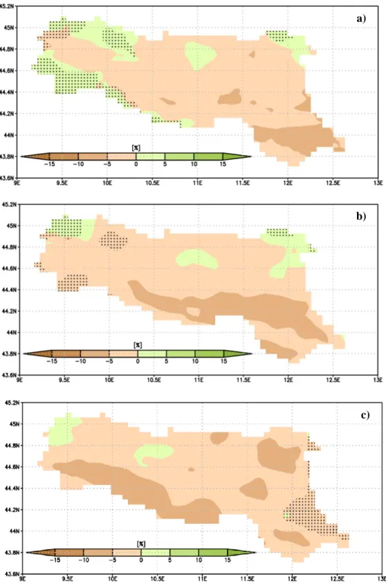
Figure 3.7 Difference in number of days during growing season with maximum temperature in the range 25–30°C between periods a) 1961–1990 vs 2011–2040 under RCP 8.5 scenario b) 1961–1990 vs 2071– 2100 under RCP 8.5 scenario c) 1961–1990 vs 2071–2100 under RCP 4.5 scenario, in the Emilia-Romagna calculated as median of 9 models. Dotted areas are statistically significant (p < 0.05) according to t-test. ... 46 Figure 3.8 Difference in number of days during growing season with maximum temperature above 30°C between periods a) 1961–1990 vs 2011–2040 under RCP 8.5 scenario b) 1961–1990 vs 2071–2100 under RCP 8.5 scenario c) 1961–1990 vs 2071–2100 under RCP 4.5 scenario, in the Emilia-Romagna calculated as median of 9 models. Dotted areas are statistically significant (p < 0.05) according to t-test ... 47 Figure 3.9 Average Cool Night Index for the period 1961–1990 in the Emilia-Romagna, calculated with historical data previously described in Chapter 2 (see 2.2.2). ... 48 Figure 3.10 Cool Night Index in the Emilia-Romagna for the periods a) 2011–2040 under RCP 8.5 scenario b) 2071–2100 under RCP 8.5 scenario and c) 2071–2100 under RCP 4.5 scenario, calculated as median of 9 models. Dotted areas are statistically significant (p < 0.05) according to t-test. ... 49 Figure 3.11 Average Huglin Index for the period 1961–1990 in the Emilia-Romagna, calculated with historical data previously described in Chapter 2 (see 2.2.2). ... 50 Figure 3.12 Huglin Index in the Emilia-Romagna for the periods a) 2011–2040 under RCP 8.5 scenario b) 2071–2100 under RCP 8.5 scenario and c) 2071–2100 under RCP 4.5 scenario, calculated as median of 9 models. Dotted areas are statistically significant (p < 0.05) according to t-test. ... 51 Figure 3.13 Average Growing Degree Day Index for the period 1961–1990 in the Emilia-Romagna, calculated with historical data previously described in Chapter 2 (see 2.2.2). ... 52 Figure 3.14 Growing Degree Day Index in the Emilia-Romagna for the periods a) 2011–2040 under RCP 8.5 scenario b) 2071–2100 under RCP 8.5 scenario and c) 2071–2100 under RCP 4.5 scenario, calculated as median of 9 models. Dotted areas are statistically significant (p < 0.05) according to t-test. ... 53 Figure 3.15 Total precipitation for the period 1961–1990 in the Emilia-Romagna, calculated with historical data previously described in Chapter 2 (see 2.2.2). ... 54 Figure 3.16 Relative difference in total precipitation during growing season between periods a) 1961– 1990 vs 2018–2027 b) 1961–1990 vs 2011–2040 c) 1961–1990 vs 2071–2100, under RCP 4.5 scenario in the Emilia-Romagna calculated as median of 9 models. Dotted areas are statistically significant (p < 0.05) according to t-test. ... 55 Figure 3.17 Relative difference in total precipitation during growing season between periods a) 1961– 1990 vs 2018–2027 b) 1961–1990 vs 2011–2040 c) 1961–1990 vs 2071–2100, under RCP 8.5 scenario in the Emilia-Romagna calculated as median of 9 models. Dotted areas are statistically significant (p < 0.05) according to t-test. ... 56 Figure 3.18 Dry Spell Index for the period 1961–1990 in the Emilia-Romagna, calculated with historical data previously described in Chapter 2 (see 2.2.2). ... 57 Figure 3.19 Difference in Dry Spell Index during growing season between periods a) 1961–1990 vs 2071– 2100 under RCP 4.5 scenario b) 1961–1990 vs 2071–2100 under RCP 8.5 scenario, in the Emilia-Romagna calculated as median of 9 models. Dotted areas are statistically significant (p < 0.05) according to t-test. ... 58 Figure 3.20 Dryness Index for the period 1961–1990 in the Emilia-Romagna, calculated with historical data previously described in Chapter 2 (see 2.2.2). ... 59 Figure 3.21 Difference in Dryness Index during growing season between periods a) 1961–1990 vs 2011– 2040 under RCP 8.5 scenario b) 1961–1990 vs 2071– 2100 under RCP 8.5 scenario c) 1961–1990 vs
2071–2100 under RCP 4.5 scenario, in the Emilia-Romagna calculated as median of 9 models. Dotted areas are statistically significant (p < 0.05) according to t-test. ... 60 Figure 4.1 Location of the studied part of Romagna area (adopted with permission from Teslić et al., 2018). ... 70 Figure 4.2 a) Linear trend of growing season mean temperature; b) Pettitt homogeneity test for a growing season mean temperature; in the studied area during the period from 1953 to 2013. ... 73 Figure 4.3 Linear trends of a) Huglin index; b) Growing degree day in the studied area during the period from 1953 to 2013. ... 74 Figure 4.4 Linear trends of a) Total precipitation; b) Dry spell index in the studied area during the period from 1953 to 2013. ... 75 Figure 4.5 Linear trends of a) grape sugar content (2001–2012); b) grape yield data (1982–2012) in the studied area. ... 76 Figure 4.6 Growing season trends of Huglin index (HI); sugar content in Sangiovese grapes (Sugar content); Dry spell index (DSI) in the studied part of Romagna area from 2001 to 2012; red line – Sugar content breaking point. ... 77 Figure 5.1 cv. Sangiovese vine development monitored over the vegetative period during the vintage 2015. T1 – winter pruning applied in December (BBCH=0); T2 – winter pruning applied in March (BBCH=0); T3 – winter pruning applied in April (BBCH=12). ... 107 Figure 5.2 cv. Sangiovese vine development progress on the 4th of May; left: T1 – winter pruning applied in December (BBCH=0); center: T2 – winter pruning applied in March (BBCH=0); right: T3 – winter pruning applied in April (BBCH=12). ... 108 Figure 5.3 Chemical composition of cv. Sangiovese must during vintage 2015. SC – Sugar content; TA – Titratable acidity; T1 – winter pruning applied in December (BBCH=0); T2 – winter pruning applied in March (BBCH=0); T3 – winter pruning applied in April (BBCH=12). ... 109 Figure 5.4 Experiment design and winemaking protocol (modified from Teslić et al., 2018). ... 112 Figure 5.5 Principal component analysis a) scores plot of Chardonnay wines according to volatile aromatic compounds; b) correlation loadings plot of Chardonnay wines with volatile aromatic compounds profile. Y1–must vinified with inoculation of Saccharomyces cerevisiae/Saccharomyces paradoxus; Y2– must vinified with sequential inoculation of Candida zemplinina and hybrid Saccharomyces
cerevisiae/Saccharomyces paradoxus; Y3–must vinified with inoculation of Saccharomyces cerevisiae;
H1–wine made with technologically mature (ratio total acidity/sugar content) Chardonnay grapes; H2– wine made with Chardonnay grapes obtained during ‘delayed harvest’; H3–wine made with blend of Chardonnay grapes obtained during ‘early green harvest’ and Chardonnay grapes obtained during ‘delayed harvest’; AceA–acetic acid; ButA–butanoic acid; HexA–hexanoic acid; EthO–ethyl octanoate; PheA–phenylethyl alcohol; IsoA–isoamyl alcohol ... 126 Figure 5.6 Sensory analysis scores of Chardonnay wines produced during vintage 2016 according to grape harvest timing. Values are the mean of 25 replicates of all samples (n=75). Statistical analysis was performed with Kruskal -Wallis test (* – p<0.05; ** – p<0.1). ... 128 Figure 5.7 Sensory analysis scores of Chardonnay wines produced during vintage 2016 according to yeast strain selection. Values are the mean of 25 replicates of all samples (n=75). Statistical analysis was performed with Kruskal -Wallis test (* – p<0.05; ** – p<0.1). ... 128 Figure 5.8 Principal component analysis a) scores plot of Chardonnay wines according to significant variables of chemical composition (without volatile aromatic compounds; b) correlation loadings plot of Chardonnay wines chemical composition (without volatile aromatic compounds) and panelist preference.
Y1–must vinified with inoculation of Saccharomyces cerevisiae/Saccharomyces paradoxus; Y2–must
vinified with sequential inoculation of Candida zemplinina and hybrid Saccharomyces
cerevisiae/Saccharomyces paradoxus; Y3–must vinified with inoculation of Saccharomyces cerevisiae;
H1–wine made with technologically mature (ratio total acidity/sugar content) Chardonnay grapes; H2– wine made with Chardonnay grapes obtained during ‘delayed harvest’; H3–wine made with blend of Chardonnay grapes obtained during ‘early green harvest’ and Chardonnay grapes obtained during ‘delayed harvest’; AAcid–acetic acid; VolAcid–volatile acidity; CafAcid–cafftaric acid; p-Cou–p-coumaric acid; TotPoly–total polyphenols; TotAci–total acidity; TAcid–tartaric acid; MAcid–malic acid; CAcid–citric acid; SAcid–succinic acid; Pref–panelist preference; pH–pH value; Alc–alcohol content. 130 Figure 5.9 Principal component analysis a) scores plot of Chardonnay wines according to significant variables of quantitative descriptive sensory analysis; b) correlation loadings plot of Chardonnay wines quantitative descriptive sensory analysis and panelist preference. Y1–must vinified with inoculation of
Saccharomyces cerevisiae/Saccharomyces paradoxus; Y2–must vinified with sequential inoculation of Candida zemplinina and hybrid Saccharomyces cerevisiae/Saccharomyces paradoxus; Y3–must vinified
with inoculation of Saccharomyces cerevisiae; H1–wine made with technologically mature (ratio total acidity/sugar content) Chardonnay grapes; H2–wine made with Chardonnay grapes obtained during ‘delayed harvest’; H3–wine made with blend of Chardonnay grapes obtained during ‘early green harvest’ and Chardonnay grapes obtained during ‘delayed harvest’; Aci–acidity; HerO–herbal odor; AlcT– alcoholic taste; AlcO–alcoholic odor; Swe–sweetness; Tcom–taste complexity; Ocom–odor complexity; FruO–fruity odor; Pref–panelist preference. ... 132 Figure 6.1 Schematic of the internal structure of the Waveguide Vector Spectrometer (adopted with permission from Teslić et al., 2017). ... 162 Figure 6.2 Correlation between antioxidative capacity and Tannins/Polyphenols ratio of studied commercial tannins. ... 166
The list of tables
Table 2.1 Mathematic definitions and classes of used BIs. ... 13 Table 2.2 Average bioclimatic indices values during the two periods (1961–1990; 1986–2015) in the Emilia-Romagna’s wine high-quality Protected Denomination of Origin appellation zones. ... 15 Table 3.1 List of all Global Climate Model/ Region Climate Model chains used in present study. ... 41 Table 4.1 Mathematic definitions and classes of used BIs. ... 71 Table 4.2 Pettitt test (PT) and Mann-Kendall test (MKT) applied to meteorological data (1953–2013) in the studied area. NS: no significant trend; *: 90% significant trend. ... 72 Table 4.3 Descriptive statistics applied to meteorological data (1953–2013) in the studied area. ... 73 Table 4.4 Pettitt test (PT) and Mann-Kendall test (MKT) applied to grape sugar content (2001–2012) and grape yield data (1982–2012) in the studied area. ... 75 Table 4.5 Descriptive statistics applied to grape yield (1982–2012) and grape sugar content data (2001– 2012) in the studied area. ... 75 Table 4.6 Standardized coefficients, adjusted R2 and p-level of multiple linear regression modeling applied to sugar content and bioclimatic indices (2001–2012); grape yield and bioclimatic indices (1982– 2012) in the studied area. ... 76 Table 5.1 Bioclimatic indices during the vintage 2015 and average bioclimatic indices values from the 1961 until the 2014. ... 107 Table 5.2 Grape yield and berry composition of cv. Sangiovese. T1 – winter pruning applied in December (BBCH=0); T2 – winter pruning applied in March (BBCH=0); T3 – winter pruning applied in April (BBCH=12). LSD: a – different from T3 with 95% significance; b – different from T1 with 90% significance; c – different from T1 with 95% significance. ... 108 Table 5.3 Chemical composition of Chardonnay grape juice obtained during vintage 2016. ... 113 Table 5.4 Bioclimatic indices during the vintage 2016 and average bioclimatic indices values from the 1961 until the 2015. ... 117 Table 5.5 Chemical composition, optical density, SO2 concentation and antioxidative capacity of Chardonnay wines produced during vintage 2016. Statistical analysis differences among trials based on one-way Anova with post-hoc test Tukey (p < 0.05; p < 0.1) are marked using different letters (see footnotes for explanation). ... 118 Table 5.6 Phenolic compounds composition in Chardonnay wines produced during vintage 2016. Statistical analysis differences among trials based on one-way Anova with post-hoc test Tukey (p < 0.05; p < 0.1) are marked using different letters (see footnotes for explanation). ... 120 Table 5.7 Organic acids composition of Chardonnay wines produced during vintage 2016. Statistical analysis differences among trials based on one-way Anova with post-hoc test Tukey (p < 0.05; p < 0.1) are marked using different letters (see footnotes for explanation). ... 121 Table 5.8 Volatile aromatic composition of Chardonnay wines produced during vintage 2016 expressed as mg/L. Statistical analysis differences among trials based on one-way Anova with post-hoc test Tukey (p < 0.1; p < 0.05) are marked using different letters (see footnotes for explanation). ... 124 Table 5.9 Volatile aromatic compounds odor activity values, description and odor threshold limits (µg/L). Odor activity values are ratio of certain compound concentration and odor threshold limit. ... 125 Table 5.10 Preference scores of Chardonnay wines. Statistical analysis of 75 replicates based on Kruskal -Wallis test (p < 0.05; p < 0.1). ... 129
Table 6.1 Red wine composition. ... 163 Table 6.2 Partial least square regression of red wine spectra for the prediction of alcohol and glycerol content from Gain and Phase spectra in the frequency range 1.6–2.1 GHz. ... 164 Table 6.3 Total polyphenols content, tannins content and DPPH radical scavenging potential of commercial tannins from different botanical origin... 166 Table 6.4 Elemental composition of commercial tannins from different botanical origin expressed as ppm. ... 167
The list of abbreviations
BI Bioclimatic index CE Catechin equivalent
CI Cool night index
Cz Candida zemplinina
DI Dryness index
DOC Controlled Denomination of Origin
DOCG Controlled and Guaranteed Denomination of Origin DOP Protected Denomination of Origin
DSI Dryness spell index DTR Diurnal temperature range
ER Emilia-Romagna
GDD Winkler index/Growing degree day GMO Genetic modification organism
HI Huglin index
LA/FM Leaf area to fruit mass ratio MKT Mann-Kendall test
ND 25–30°C Number of days with max temperature in the range 25–30°C ND > 30C° Number of days with max temperature >30°C
OAV Odor activity value
OIV International organization of vine and wine PCA Principal component analysis
PLS Partial least square
PreSc Preference scores
PT Pettitt test
RCM Regional Climate Models
RCP Representative concentration pathway RMSE Root mean square error
Sc Saccharomyces cerevisiae
Sp Saccharomyces paradoxus
Tmax Growing season maximum temperature Tmean Growing season mean temperature
Tmin Growing season minimum temperature Tprec Total precipitation
WVS Waveguide Vector Spectrometer
1 | P a g e
CHAPTER 1
2 | P a g e
1 Introduction and Project aim
1.1 Introduction
‘Climate change’ is a change in the weather patterns that can be detected (e.g. using statistical test) as deviation in the mean and/or the variability of its features, which is persistent for the certain period (decades or longer). These deviations refer to any changes in the weather patterns, whether they occurred due to natural factors (e.g. volcano activities, forest fires, El Niño) or anthropogenic factors (e.g. exhaust gases from cars and factories) (IPCC, 2007). Apart from constantly present changes in weather patterns due to natural factors (e.g. five major ice ages), since the middle of the 20th century exist also considerable influence of anthropogenic factors (Fig 1.1). Influence of climate change may be manifested though many direct or indirect consequences (e.g. increase of Global temperature, increased risk of droughts, accelerated ice cape melting), which further alter vast number of ecosystems on the Earth.
Figure 1.1 Contribution of natural (blue) and anthropogenic (red) factors to the observed (black) and
simulated (gray) mean Global temperature increase (modified from Huber and Knutti, 2011).
Vitis vinifera is highly sensitive to climate conditions (Fraga et al., 2012; Gladstones, 2011; Holland
and Smith, 2014)such as air temperature and precipitation, therefore climate change can modify grape and wine composition to large extent. Sensitivity to climate characteristic is reflected by narrow areas suitable for the high-quality wines production, often determined by growing season isotherms that vary from too cold (<12°C) to too hot (>22°C) (Jones, 2006) (Fig. 1.2).
3 | P a g e
Figure 1.2 Global wine regions and 12–22°C growing season temperature zones (April–October in the
Northern Hemisphere and October–April in the Southern Hemisphere) (adopted with permission from Jones, 2012).
Hypothesis that climate conditions, in particular temperature (Jones, 2012), have strong influence on viticulture is also supported by historical evidence of vine-producing existence in the north coastal zones of the Baltics and southern England from 900 to 1300, due to the higher temperatures in that period (Gladstones, 1992), and also production fade from the same regions making them inadequate due to the dramatic decrease of temperature, starting from the 14th until the 19th century (Jones et al., 2005) (Fig
1.3).
Figure 1.3 Standardized temperature variation in central England during last thousand years (modified
from Crowley and Lowery, 2000).
The influence of the climate change on wine sector is depending on vast number of direct and indirect variables such are air temperature (Neethling et al., 2012), precipitations (see 4.2.2.2), atmosphere level of CO2 (Kizildeniz et al., 2015), ultraviolet (UV-B) radiation (Schultz, 2000), planted grape varieties
(Tomasi et al., 2011), application of adaptation techniques and husbandry practices (Hunter et al., 2016; Palliotti et al., 2014; Varela et al., 2015), topography and soil characteristics (Fraga et al., 2014a) etc. Combination of all mentioned factors is in greater or lesser percent unique for each grape producing region, which is evident in many published works related to this topic (Bonnefoy et al., 2013; Fraga et
4 | P a g e
al., 2014b Hall and Jones, 2010; Lorenzo et al., 2013; Resco et al., 2016; Vršić et al., 2014), thus there is a need to examine also currently unstudied areas such as the traditional wine region Emilia-Romagna (Italy) due to its great importance at a national and international level. Assessment of climate change may be conducted whether for the past or the future, whereas both parts are required to fully understand climate change trends and gather information which later serve as a tool to develop adaptation strategies. The final outcome and consequences of climate change influence on wine industry could rather be positive or negative. Negative consequences on wine industry are manifested as crop load reduction (Ramos and Martínez-Casasnovas, 2010), production of unbalanced wines with excessive alcohol (Jones et al., 2005), utilization of additional investment expenses in mitigation technologies, reduction of anthocyanins (Mori et al., 2007),lower must acidity (Godden et al., 2015) etc. On the contrary, in some high quality wine regions, such as Chianti (Italy), Bordeaux and Burgundy (France), Barossa and Margaret River (Australia), warming resulted in increasing trends of wine vintage ratings over the second half of the 20th century (Jones et al., 2005). Furthermore, warming in future decades may translocate zones with optimal growing season mean temperature (12–22°C) polewards, towards the coast and higher elevations (Jones, 2012) and transform non-traditional wine producing zones to suitable for grape cultivation(Bardin-Camparotto et al. 2014).
The wine and grape industry is widely spread over the world with approximately 7534 Kha of planted vineyard surfaces worldwide, with 274 MhL of wine and must production per year (harvest 2015). Even though, wine consumption was reduced worldwide after economic crisis in 2008, total volume of exported wine, same as the total value of exports is steadily growing from 2000’s on a globe scale, suggesting that sustainable winemaking industry is an important factor for the economic stability in counties which are the largest wine exporters (France, Italy, Spain) (OIV, 2016). Nowadays, a sustainable wine industry in environment of accelerated climate change becomes a great challenge, thus it is necessary to develop appropriate adaptation techniques to mitigate upcoming events. In literature, there are already a various adaptation techniques that can be divided into four principal groups: (i) viticulture techniques, (ii) pre-fermentation techniques, (iii) biotechnological techniques and (iv) post-fermentation techniques. However, due to high diversity of climatic conditions over entire wine industry and everlasting trend to decrease cost of production and increase quality of final products there is a need to further develop new mitigation techniques and to examine synergistic effect of existing techniques.
1.2 Project aim
The aim of this PhD thesis titled: ‘Climate change vs Wine industry in the Emilia-Romagna: Assessment
of the climate change, influence on wine industry and mitigation techniques’ is to examine climate change
trends in the Emilia-Romagna (ER) during both, past and future decades, with appropriate meteorological data base and suitable statistic tools. To identify the link, if any, between climate trends and grape quality/quality parameters and to develop new adaptation techniques to moderate the influence of climate change on wine industry.
5 | P a g e
To achieve this aim, several experiments were designed as followed:
I. Climatic shifts in the ER’s high-quality wine production areas – covers examination of climate changes by calculating bioclimatic indices (BIs) for currently well-established high-quality wine production areas of the ER during the period 1961–2015; examination of climate changes in currently grape non-cultivated areas of the ER to identify, from climatological aspect, a new suitable area for grape production in the ER.
II. Projections of climatic shifts in the ER wine production areas – covers examination of climate projections in the periods 2018–2027, 2011–2040 and 2071–2100 under two possible scenarios (Representative concentration pathway (RCP) 4.5 and RCP 8.5) by calculating BIs for currently well-established high-quality wine production areas of the ER during.
III. Influence of climate change on grape yield and sugar content of Sangiovese grapes from the studied part of Romagna – covers assessment of climate change trends over 61 years (from 1953 to 2013) in the studied area by calculating BIs; relation between BIs and grape sugar content from seven wineries during the period 2001–2012; relation between BIs and grape yield during the period 1982–2012.
IV. Development of new adaptation techniques to climate change.
a. Effect of late winter pruning on Sangiovese grape berry composition from organic management – covers examination of late winter pruning as potential technique to moderate effect of increasing total soluble solids must concentration in organic Sangiovese grapes caused by warmer and/or drier climatic conditions.
b. Combination of viticulture and biotechnological techniques as a method to reduce alcohol content and pH – covers assessment of possibilities to use viticulture and biotechnological techniques as a combined method to mitigate negative impact of hot and dry vintages (e.g. excessive ethanol concentration and high pH) on Chardonnay wines.
V. Development of analytical method to evaluate wine parameters affected by climate change and analytical profiling of additives to face climate change.
a. Development of method using Waveguide Vector Spectrometer to examine alcohol and glycerol content of red wines.
b. Analytical profiling of commercial tannins by ICP-MS and spectrophotometric methods to identify potential additives in winemaking that could be used during hot vintages.
6 | P a g e
1.3 References
Bardin-Camparotto, L., Blain, G.C., Júnior, M.J.P., Hernandes, J.L., Cia, P., 2014. Climate trends in a non-traditional high quality wine producing region. Bragantia 73, 327–334.
Bonnefoy, C., Quenol, H., Bonnardot, V., Barbeau, G., Madelin, M., Planchon, O., Neethling, E., 2013. Temporal and spatial analyses of temperature in a French wine-producing area: The Loire Valley. International Journal of Climatology 33, 1849–1862.
Crowley, T., Lowery, T., 2000. How warm was the mediaval warm preriod? A Journal of the Human Environment 29, 51–54.
Fraga, H., Malheiro, A.C., Moutinho-Pereira, J., Cardoso, R.M., Soares, P.M.M., Cancela, J.J., Pinto, J.G., Santos, J.A., 2014. Integrated analysis of climate, soil, topography and vegetative growth in Iberian viticultural regions. PLoS ONE 9.
Fraga, H., Malheiro, A.C., Moutinho-Pereira, J., Santos, J.A., 2014. Climate factors driving wine production in the Portuguese Minho region. Agricultural and Forest Meteorology 185, 26–36. Fraga, H., Malheiro, A.C., Moutinho-Pereira, J., Santos, J.A., 2012. An overview of climate change
impacts on European viticulture. Food and Energy Security 1, 94–110.
Gladstones, J., 2011. Wine, Terroir and Climate Change. Wakefield Press, Kape Town, Australia. Gladstones, J., 1992. Viticulture and Enviroment. Winetitles, Adelaide, Australia.
Godden, P., Wilkes, E., Johnson, D., 2015. Trends in the composition of Australian wine 1984–2014. Australian Journal of Grape and Wine Research, 21, 741–753.
Hall, A., Jones, G. V, 2010. Spatial analysis of climate in winegrape-growing regions in Australia. Australian Journal of Grape and Wine Research 16, 389–404.
Holland, T., Smit, B., 2014. Recent climate change in the Prince Edward County winegrowing region, Ontario, Canada: Implications for adaptation in a fledgling wine industry. Regional Environmental Change 14, 1109–1121.
Huber, M., Knutti, R., 2011. Anthropogenic and natural warming inferred from changes in Earth’s energy balance. Nature Geoscience 5, 31–36.
Hunter, J.J., Volschenk, C.G., Zorer, R., 2016. Vineyard row orientation of Vitis vinifera L. cv.
Shiraz/101-14 Mgt: Climatic profiles and vine physiological status. Agricultural and Forest
Meteorology 228–229, 104–119.
IPCC, 2007. Climate Change 2007 Synthesis Report, Intergovernmental Panel on Climate Change [Core Writing Team, Pachauri, R.K and Reisinger, A. (Eds.)]. IPCC, Geneva, Switzerland.
7 | P a g e
Jones, G. V, 2012. Climate, grapes, and wine: Structure and suitability in a changing climate, in: Bravdo, B., Medrano, H. (Eds.), Proceedings of the 28th IHC – IS Viticulture and climate: Effect of climate change on production and quality of grapevines and their products. Acta Horticulturae, Lisbon, Portugal, pp 19–28.
Jones, G. V, 2006. Climate and Terroir: Impacts of Climate Variability and Change on Wine, in: Macqueen, R.W., Meinert, L.D. (Eds.), Fine Wine and Terroir – The Geoscience Perspective. Geological Association of Canada, Newfoundland, Canada.
Jones, G. V, White, M.A., Cooper, O.R., Storchmann, K., 2005. Climate change and global wine quality. Climatic Change 73, 319–343.
Kizildeniz, T., Mekni, I., Santesteban, H., Pascual, I., Morales, F., Irigoyen, J.J., 2015. Effects of climate change including elevated CO2 concentration, temperature and water deficit on growth, water status, and yield quality of grapevine (Vitis vinifera L.) cultivars. Agricultural Water Management 159, 155–164.
Lorenzo, M.N., Taboada, J.J., Lorenzo, J.F., Ramos, A.M., 2013. Influence of climate on grape production and wine quality in the Rías Baixas, north-western Spain. Regional Environmental Change 13, 887–896.
Mori, K., Goto-Yamamoto, N., Kitayama, M., Hashizume, K., 2007. Loss of anthocyanins in red-wine grape under high temperature. Journal of Experimental Botany 58, 1935–1945.
Neethling, E., Barbeau, G., Bonnefoy, C., Quénol, H., 2012. Change in climate and berry composition for grapevine varieties cultivated in the Loire Valley. Climate Research 53, 89–101.
OIV, 2016. State of the vitiviniculture world market. OIV, Paris, France.
Palliotti, A., Tombesi, S., Silvestroni, O., Lanari, V., Gatti, M., Poni, S., 2014. Changes in vineyard establishment and canopy management urged by earlier climate-related grape ripening: A review. Scientia Horticulturae 178, 43–54.
Ramos, M.C., Martínez-Casasnovas, J.A., 2010. Soil water balance in rainfed vineyards of the Penedès region (northeastern Spain) affected by rainfall characteristics and land levelling: Influence on grape yield. Plant and Soil 333, 375–389.
Resco, P., Iglesias, A., Bardají, I., Sotés, V., 2016. Exploring adaptation choices for grapevine regions in Spain. Regional Environmental Change 16, 979–993.
Schultz, H.R., 2000. Climate change and viticulture: A European perspective on climatology, carbon dioxide and UV-B effects. Australian Journal of Grape and Wine Research 6, 2–12.
Tomasi, D., Jones, G. V, Giust, M., Lovat, L., Gaiotti, F., 2011. Grapevine Phenology and Climate Change: Relationships and Trends in the Veneto Region of Italy for 1964–2009. American Journal of Enology and Viticulture 62, 329–339.
8 | P a g e
Varela, C., Dry, P.R., Kutyna, D.R., Francis, I.L., Henschke, P.A., Curtin, C.D., Chambers, P.J., 2015. Strategies for reducing alcohol concentration in wine. Australian Journal of Grape and Wine Research 21, 670–679.
Vršič, S., Šuštar, V., Pulko, B., Šumenjak, T.K., 2014. Trends in climate parameters affecting winegrape ripening in northeastern Slovenia. Climate Research 58, 257–266.
9 | P a g e
CHAPTER 2
Climate change in the Emilia-Romagna’s DOP appellation areas
(1961–2015)
10 | P a g e
2 Climate change in the Emilia-Romagna’s high-quality wine DOP
appellation areas (1961–2015)
Teslić, N., Vujadinović, M., Ruml, M., Antolini, G., Vuković, A., Parpinello, Giuseppina P., Ricci, A., Versari, A.,
2017. Climatic shifts in high quality wine production areas, Emilia Romagna, Italy, 1961–2015. Climate Research 73, 195–206
Versari, A., Ricci, A., Teslić, N., Parpinello G.P., 2017. Climate change trends, grape production, and potential alcohol concentration in Italian wines. In Proceedings of the SIAVEN Symposium. Chile
2.1 Introduction
As mentioned before grape production is strongly affected by climate variables (Fraga et al. 2012a), thus climate change may modify grape and wine composition to a great extent. However, due vast number of relevant climatic factors (e.g. temperature) and non-climatic factors (e.g. topography) the magnitude of climate change may diverse among wine regions (Jones et al., 2005). This was confirmed by Jones et al. (2005) that reported a significant growing season temperature trends for the majority of Europe and North-America wine regions during the last 50 years of the 20th century, with an average increase of 1.26°C. However, authors also reported the lack of statistically significant temperature trends for the majority of Southern Hemisphere wine regions. Thus, despite the importance of the global climate change trend, from the viticulturist/winemaker point of view it is also important to understand and examine regional climate change trends in order appropriately adapt to potential upcoming climate changes that could have impact on grape and wine composition. Therefore, climate change examination on regional level is particularly important for currently unstudied areas, such as the traditional Italian wine region ER due to its great importance at a national and international level.
Since the magnitude of climate modifications depends on mutual interaction of climatic and non-climatic variables, examinations of simple temperature and precipitation values are insufficient to explain climate change on regional level. Thus, certain BIs developed for effective monitoring of climate change in wine regions have to be used. Whereas computation of commonly used BIs allows easier comparison of climate characteristics and climate change shifts between wine regions. These BIs may be divided into three groups: (i) BIs derived from a single climatic variable (e.g. minimum temperatures during September – Cool night index (Tonietto, 1999)); (ii) BIs derived from two or more climatic variables (e.g. maximum and mean temperatures from April to September – Huglin index (Huglin, 1978)); (iii) BIs derived from climatic and non-climatic variables (e.g. monthly precipitation and evaporation of bare soil – Dryness index (Tonietto and Carbonneau, 2004)). In the last two decades, BI were computed by spatially interpolated meteorological data sets (Fraga et al., 2012b; Hall and Jones, 2010) or data sets directly from the meteorological stations (Duchêne and Schneider, 2005; Tomasi et al., 2011). Meteorological data sets from meteorological stations are surely a valuable tool for the regional climate change examination. However, spatially interpolated data sets may allow more precise estimates of climate variables at locations distant from the measuring meteorological stations. Furthermore, spatially interpolated data sets have often temporally complete series which allows easier implementation
11 | P a g e
(Haylock et al., 2008). The suitability of the spatially interpolated data sets for the regional climate change studies is strongly related to spatial resolution. This is of the paramount importance due to often complex topography of the grape cultivation regions, where data sets with relatively low spatial resolution provided by global climate models (up to 250 km) (Jones et al., 2005; Webb et al., 2007) or regional climate models (up to 25 km) (Andrade et al., 2014; Lorenzo et al., 2013)may be inadequate to present vineyard climate characteristics. Therefore, high-resolution, spatially interpolated climatic data (up to 5 km) (Fraga et al., 2014; Lorenzo et al., 2016) may be a valuable tool for the regional climate change examination of the grape growing areas.
Italyis one of the top world’s wine producer with 49.5 106 hL of produced wine during the vintage 2015 and 682 000 ha of the total vineyard area (OIV, 2016). Total value of all exported wine reached 5.35 109 € during the 2015 (OIV, 2016), whereas approximately 50% of the total value of all exported Italian wine during 2015 was obtained by trading high-quality wine with Protected Denomination of Origin (DOP) (www.italianwinecentral.com). Therefore, high-quality wine industry affects the economic, social and cultural aspects of Italy to a great extent. Thus, the aim of this experiment was to ascertain the appearance, if any, of climatic change that could affect the winemaking industry in DOP appellation zones in the ER.
2.2 Materials and Methods
2.2.1 Study region
The traditional viticulture region ER is located in the northern Italy and stretches from ~ 43° 80’ to 45° 10’ N latitude and ~ 9° 20’ to 12° 75’ E longitude. Rich pedological and climatic diversity caused by the impact of the Adriatic Sea to the east and the mountains to the south, create a unique ‘terroir’ suitable for the cultivation of several grape varieties, both international and autochthonous. The ER counts about 55 000 ha of vineyards, representing 8.1% of the total Italian vineyard surface, with the main grape varieties such as Trebbiano Romagnolo white grape that covers 30.4%, Lambrusco red grape 17.7%, Sangiovese red grape 15.5%, Ancellota red grape that covers 7.9% of the total ER vineyard surfaces (Pollini et al., 2013). The total ER wine production is estimated on 7.91 106 hL during vintage 2014, placing the ER as the 2nd winemaking region with 18% of the total Italian wine production by volume. A considerable volume of the total ER’s wine production (15.9%, vintage 2014) is high-quality DOP (Protected Denomination of Origin) wines, which are divided into subgroups, DOCG (Controlled and Guaranteed Denomination of Origin) and DOC (Controlled Denomination of Origin) wines. The production of the DOP wines is widespread over the entire ER region except for the mountain zones and certain northeastern and northwestern zones (Fig. 2.1).
12 | P a g e
Figure 2.1 Location DOC (Controlled Denomination of Origin) and DOCG (Controlled and Guaranteed
Denomination of Origin) grape production areas in the Emilia-Romagna (modified from www.enotecaemiliaromagna.it).
2.2.2 Meteorological data and bioclimatic indices
The experiment was conducted using a high-resolution gridded climate data provided by the Regional Agency for Prevention, Environment and Energy of the Emilia-Romagna (www.arpae.it). Gridded meteorological data for the period 1961–2015 were obtained from precipitation (254 locations) and temperature (60 locations) time series, preliminarily checked for quality, temporal homogeneity and synchronicity. The daily climate data were interpolated on a 5 x 5 km grid, by the algorithms as described in details elsewhere (Antolini et al., 2016). Algorithms consider topography (lapse rate examination, including thermal inversions; topographic barriers; topographic relative position), land use (urban fraction), and a day-by-day error minimizing procedure for the examination of the interpolation parameters. Specific BIs were computed for the DOP appellation viticulture zones over the two periods: 1961–1990, as a standard climatological period, and 1986–2015, as the latest 30-year time-series. The BIs used for this experiment were calculated as presented in Table 2.1.
13 | P a g e
Table 2.1 Mathematic definitions and classes of used BIs.
Bioclimatic index
Mathematical definition
Classes Temperature related indices
Growing season mean temperature (Tmean)1 ∑
Tn – Mean air temperature (°C) N – Number of days Too cool: < 12 Cool: 12–15 Intermediate: 15–17 Warm: 17–19 Hot: 19–21 Very Hot: 21–22 Too Hot: > 22
Number of days with max temperature in the
range 25–30°C (ND 25–30°C)2
∑
ND 25–30°C – Number of days with max temperature in the range 25–30°C
Number of days with max temperature in the range 25–
30°C (ND 25–30°C)2
Number of days with max temperature > 30°C (ND > 30°C)2 ∑ ND > 30°C – Number of days with max temperature > 30°C
Number of days with max temperature > 30°C (ND >
30°C)2
Cool night index(CI)3 ∑
Tm – Min air temperature (°C) N – Number of days
Warm nights: > 18 Temperate nights: 14–18 Cool nights: 12–14 Very cool nights: < 12
Huglin index (HI)4
∑
Tx – Max air temperature (°C)
Tn – Mean air temperature (°C)
k – Length of the day correction coefficient
Very warm: > 300000 Warm: 2400−30000 Temperate warm: 2100−2400 Temperate: 1800−21000 Cool: 1500−1800 Very cool: < 1500
14 | P a g e
Bioclimatic index
Mathematical definition
Classes
Growing degree day (GDD)5,6
∑
Tm – Min air temperature (°C) Tx – Max air temperature (°C)
Too hot: > 27000000 Region V: 2222−2700 Region IV: 1944−2222 Region III: 1667−1944 Region II: 1389−1667 Region I: 850−1389 Too cool: < 850
Precipitation related indices
Total precipitation (Tprec) ∑ P – Precipitation (mm) -
Dry spell index (DSI)7
∑
ND < 1 mm – Number of days with precipitation < 1mm
-
Temperature, precipitation and non-climatic variables related indices
Dryness Index (DI)4
∑
W0 – initial soil moisture (200 mm)
Pm – monthly precipitation
ET – Water loss through transpiration
ES – Bare soil evaporation
PET – Potential evaporation
Humid : > 150
Moderately dry: 50÷150 Sub-humid: -100÷50 Very dry: < -100
a –Plant radiation absorption coef (a= 0.1,0.3,0.5 in April, May, June–September, respectively) Nefprec – Monthly effective soil
evaporation
N – Number of days in month
1(Fraga et al., 2014), 2(Ramos et al., 2008), 3(Tonietto, 1999), 4(Tonietto and Carbonneau, 2004), 5(Hall and
15 | P a g e
2.3 Results and Discussion
Narrow areas suitable for the production of high-quality wines are often determined by growing season isotherms that ranges from too cool until too hot (12°C<Tmean>22°C) (Fraga et al., 2014). Average Tmean in the ER’s high-quality wine production areas during the periods 1961–1990 and 1986–2015 was 17.64 and 18.72°C, respectively (Table 2.2). However, even if average Tmean in the Emilia-Romagna’s DOP zones was characterized as ‘warm’ during the second period (1986–2015), in certain DOP zones of the ER, Tmean was characterized as ‘hot’ during the same period (Teslić et al., 2017).
Table 2.2 Average bioclimatic indices values during the two periods (1961–1990; 1986–2015) in the
Emilia-Romagna’s wine high-quality Protected Denomination of Origin appellation zones.
The increase of Tmean suggests different impact on regional viticulture suitability and production of high-quality wines. In particular, lesser appearance of vintages with ‘warm’ Tmean particularly after 2000’s (Fig.
2.2), which are optimal for Sangiovese, one of the main red cultivars in the ER (Pollini et al., 2013), may
induce viticulturists to cultivate later maturing grapevine varieties in order to adapt to upcoming warming conditions that are expected for the entire northern Italy (Ruml et al., 2012). Grape varieties that may be potentially suitable for cultivation during the future decades in DOP areas of ER region include Grenache, Carignane, Zinfandel and Nebbiolo (Fig. 2.3).
Figure 2.2 Average mean growing season temperature in the Emilia-Romagna’s wine high-quality
Protected Denomination of Origin appellation zones from 1961 until 2015.
Furthermore, as a direct consequence of increasing temperatures, an average number of days exceeding 30°C increased in the ER’s DOP zones in the second period (45.60 days; 1986–2015) comparing to the first period (24.77 days; 1961–1990), (Table 2.2). Inversely, an average number of days with maximum
Period Tmean [°C] CI [°C] ND25–30°C [days] ND>30°C [days] HI [units] GDD [units] Tprec [mm] DSI [days] DI [mm] 1961–1990 17.64 13.19 61.42 24.77 2048.35 1663.67 472.56 165.00 99.48 1986–2015 18.72 13.31 60.04 45.60 2299.90 1888.84 469.04 165.18 71.52
16 | P a g e
temperatures was approximately constant in the ER’s DOP zones (Table 2.2). These changes may affect vine photosynthesis and growth process, since days with maximum temperature in the range of 25–30°C is optimal for the vine photosynthesis (Carbonneau et al., 1992). On the other hand, a certain number of days exceeding 30°C may induce vine heat stress, premature véraison, berry abscission, reduced flavor development and enzyme activation (Mullins et al., 1992). During the 21st century, daily maximum temperature in the vegetative period may even exceed 45°C, reaching upper-temperature limit for the photosynthesis process (Greer and Weedon, 2012), and having a negative impact on the grape berry composition and crop load.
Figure 2.3 Optimal mean growing season temperatures (Tmean) for the cultivation of certain grape varieties. The range of the Tmean for two periods (1961–1990, black; 1986–2015, red) presents standard deviation of Tmean during respective periods (modified from Jones, 2006).
In the ER’s DOP zones, CI which is related to the grape’s synthesis of anthocyanins was approximately constant in the both periods (Table 2.2), and nights were characterized as ‘cool’ during most of the vintages in the last 55 years (Fig. 2.4). Several studies (Kliewer, 1977; Tonietto and Carbonneau, 1998) reported a positive effect of the night temperatures in an approximate range of 10–15°C on anthocyanin accumulation during the berry maturing period. Hence, obtained results in presented experiment suggested optimal night conditions for cultivation of red grape varieties which are used for red and rosé wine production that represents 55% of the total ER wine production (Pollini et al., 2013).
17 | P a g e
Figure 2.4 Average Cool night index in the Emilia-Romagna’s wine high-quality Protected
Denomination of Origin appellation zones from 1961 until 2015.
Average thermal accumulation in the ER’s DOP areas presented as HI, was 2048.35 and 2299.90 units during the period 1961–1990 and 1986–2015, respectively (Table 2.2). During the first period (1961– 1990) vintages in the ER’s DOP were mainly characterized as ‘temperate/warm temperate’ according to Huglin classification (Fig. 2.5). However, due to warming, during the second period (1986–2015) same areas were characterized as ‘warm temperate/warm’ (Fig. 2.5). This increase of thermal accumulation will most likely continue in the upcoming decades. It is predicted that the entire northern Italy, including the ER DOP zones, could be characterized as ‘warm’ (according to Huglin classification) wine region in the upcoming decades (2041–2070; A1B scenario) (Fraga et al., 2013). In general, the magnitude of these changes will strongly depend on a level of anthropogenic carbon emissions into the atmosphere during the upcoming decades. Higher temperatures and consequently higher thermal accumulation may have a negative impact on grape/wine quality (see 4.1.1–4.1.6).
Figure 2.5 Average Huglin index in the Emilia-Romagna’s wine high-quality Protected Denomination of