Behaviour and design of composite steel concrete slabs

(1)

POLITECNICO DI MILANO

SCUOLA DI INGEGNERIA CIVILE, AMBIENTALE E

TERRITORIALE

CORSO DI LAUREA MAGISTRALE IN INGEGNERIA CIVILE-

CIVIL ENGINEERING

BEHAVIOUR AND DESIGN OF COMPOSITE STEEL-CONCRETE

SLABS

Relatore: Prof. Massimiliano Bocciarelli Relatore: Prof. Gianluca Ranzi

Tesi di laurea magistrale di:

Riccardo Luzzi Matr. 819034

(2)

To my family,

for its support throughout my life

(3)

1

Figures

Fig 1.1 Composite slabs ... 15

Fig 1.2 Propped slab ... 16

Fig 1.3 Elements of a composite slab and notations ... 16

Fig 1.4 Examples of steel sheeting profiles ... 17

Fig 1.5 Types of shear connections ... 18

Fig 1.6 Shear-bond failure (Porter , Ekberg , 1975) ... 20

Fig 1.7 Typical set-up for testing slab elements (Porter , Ekberg , 1975) ... 21

Fig 1.8 Shear-bond failure relationship (Porter , Ekberg, 1975) ... 22

Fig 1.9 Horizontal force equilibrium for steel profile (Stark, Brekelmans, 1990) ... 23

Fig 1.10 Moment-distance from support on partial shear connection strength model (Star , Brekelmans, 1990) ... 24

Fig 1.11 Shrinkage deflection theory (Montgomery, Kulak, Shwartsburd, 1983) ... 25

Fig 1.12 Typical shrinkage profile specimens. (Gilbert, Bradford, Gholamhoseini, Chang, 2011) ... 27

Fig 1.13 Qualitative uniform shrinkage distribution for slab exposed on both sides . 28 Fig 1.14 Qualitative linear shrinkage distribution for composite slab. (Ranzi, Leoni, Zandonini, 2012) ... 29

Fig 2.1 Concrete strain components (Gilbert, Ranzi, 2010) ... 31

Fig 2.2 Time-stress history (Gilbert, Ranzi, 2010) ... 38

Fig 2.3 Time discretization (Gilbert, Ranzi, 2010) ... 38

Fig 2.4 Composite samples for shrinkage measurement (Al-Deen, Ranzi, 2015b) .... 42

Fig 2.5 Total long-term measured at different instances in time through the cross-section ... 42

Fig 2.6 Strain variables describing non-uniform free shrinkage on composite slabs . 44 Fig 2.7 The metal sheeting ... 47

Fig 2.8 Elastic-plastic constitutive law of steel ... 47

(7)

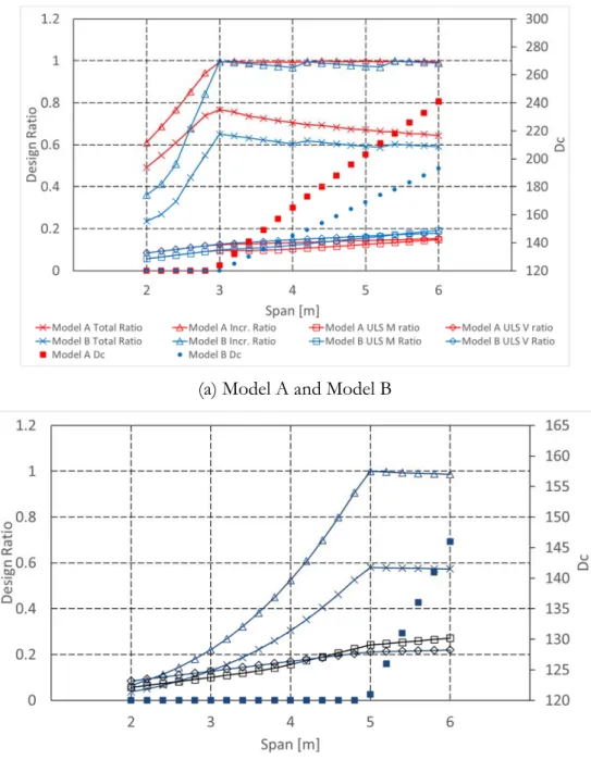
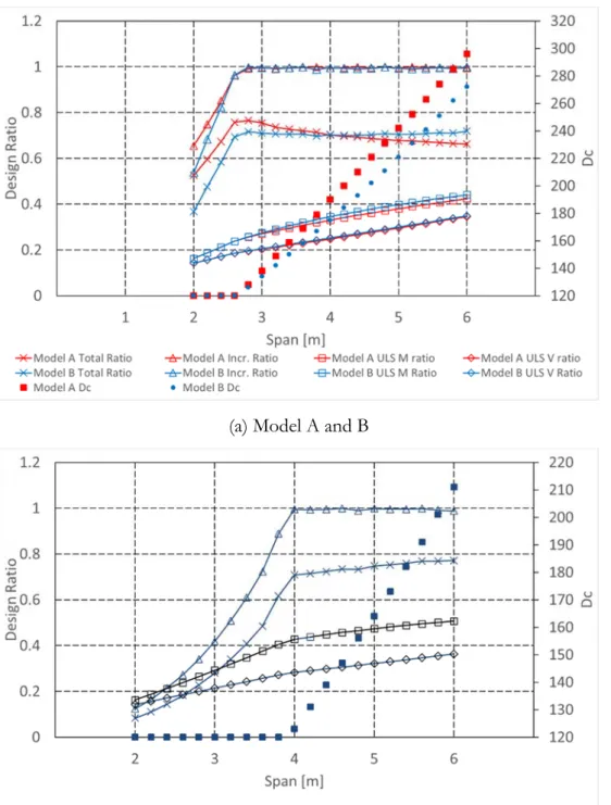
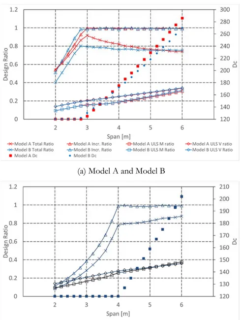
5 Fig 3.1 Stress distribution for sagging bending if the neutral axis is above the steel sheeting (Draft AS2327) ... 52 Fig 3.2 Stress distribution for sagging bending if the neutral axis is in the steel sheeting (Draft AS2327) ... 52 Fig 3.3 Static configuration of the composite slab ... 54 Fig 3.4 Stress distribution for the computation of cracked cross-section’s properties ... 59 Fig 3.5 Geometry of the profiled sheeting used in the parametric study ... 61 Fig 3.6 Design ratios and thickness depth for a propped slab with metal sheeting 1 in the case of model A and model B (Q = 3 kPa, tincr=28 days) ... 63 Fig 3.7 Design ratio and thickness depth for a propped slab with metal sheeting 1 in the case of model C (Q = 3 kPa, tincr=28 days) ... 65 Fig 3.8 Design ratios and thickness depth for an unpropped slab with metal sheeting 1 for the models A, B and C (Q = 3 kPa, tincr=28 days) ... 66 Fig 3.9 Design ratios and thickness depth for a propped slab with metal sheeting 2 for the models A, B and C (Q = 3 kPa, tincr=28 days) ... 67 Fig 3.10 Design ratios and thickness depth for an unpropped slab with metal sheeting 2 for the models A, B and C (Q = 3 kPa, tincr=28 days) ... 68 Fig 3.11 Design ratios and thickness depth for a propped slab with metal sheeting 1 for the models A, B and C (Q = 3 kPa, tincr=56 days) ... 69 Fig 3.12 Design ratios and thickness depth for a propped slab with metal sheeting 1 for the models A, B and C (Q = 3 kPa, tincr=84 days) ... 70 Fig 3.13 Design ratios and thickness depth for a propped slab with metal sheeting 1 without considering the incremental limit as a design criterion (Q = 3 kPa) ... 72 Fig 3.14 Comparisons among thickness depth computed using the models A, B and C for the profile 1 (Q = 3 kPa) ... 73 Fig 3.15 Comparisons among thickness depth computed using the models A, B and C for the profile 2 (Q = 3 kPa) ... 74 Fig 3.16 Comparisons among incremental deflection computed using the models A, B and C for the profile 1 (Q = 3 kPa) ... 75

(8)

6 Fig 3.17 Comparisons among incremental deflection computed using the models A, B and C for the profile 1 (Q = 3 kPa), without considering the minimum slab thickness

limit for 120 mm ... 76

Fig 3.18 Comparisons among incremental deflection computed using the models A, B and C for the profile 2 (Q = 3 kPa) ... 76

Fig 3.19 Comparisons among incremental deflection computed using the models A, B and C for tincr=56 days (Q = 3 kPa, profile 1) ... 77

Fig 3.20 Comparisons among incremental deflection computed using the models A, B and C for tincr=84 days (Q = 3 kPa, profile 1) ... 77

Fig 3.21 Comparisons among total deflection computed using the models A, B and C for the profile 1 (Q = 3 kPa) ... 78

Fig 3.22 Comparisons among total deflection computed using the models A, B and C for the profile 2 (Q = 3 kPa) ... 79

Fig 4.1 Displacement field ... 82

Fig 4.2 Member loads and nodal actions ... 84

Fig 4.3 Shape functions used for the approximation of u ... 88

Fig 4.4 Shape functions used for the approximation of v ... 89

Fig 4.5 7-dof Euler Bernoulli beam ... 89

Fig 4.6 Newton-Raphson Method (Ranzi, Gilbert, 2014) ... 93

Fig 4.7 Concrete strip area ... 100

Fig 4.8 Cross-sectional discretization and stress diagram ... 101

Fig 4.9 Circular segment's area ... 102

Fig 4.10 Geometric quantities of the metal sheeting ... 102

Fig 5.1 Comparison on the designed depth between Code and FEA for profile 1, with incremental check (Q=3 kPa) ... 106

Fig 5.2 Comparison on the designed depth between Code and FEA for profile 1, with no incremental check (Q=3 kPa) ... 106

Fig A- 1 Comparisons among total deflection computed using the models A, B and C for the profile 1 ... 127

(9)

7 Fig A- 2 Comparisons among total deflection ratio computed using the models A, B and C for the profile 2 ... 128 Fig A- 3 Comparisons among total deflection computed using the models A, B and C for the profile 1 ... 129 Fig A- 4 Comparisons among total deflection computed using the models A, B and C for the profile 2 ... 130 Fig A- 5 Comparison on the designed depth between Code and FEA for profile 2, with incremental check (Q=3 kPa) ... 131 Fig A- 6 Comparison on the designed depth between Code and FEA for profile 2, with no incremental check (Q=3 kPa) ... 131

(10)

8

Tables

Table 2-1 Validation of the linear shrinkage ... 45 Table 2-2 Geometric properties of the profiled steel sheeting ... 48 Table 3-1 Load combinations for the evaluation of deflections in propped construction ... 55 Table 3-2 Load combinations for the evaluation of deflections in unpropped construction ... 55 Table 4-1 Function arguments and weighting factors for the Gauss-Legendre formulae (Ranzi, Gilbert, 2014) ... 97 Table 4-2 Validation of the finite element mode ... 103 Table 4-3 Validation of the finite element model ... 104 Table 5-1 Comparison on the incremental deflection between Code and FEA for profile 1 (linear shrinkage, Q=3 kPa) ... 108 Table 5-2 Comparison on the total deflection between Code and FEA for profile 1 (linear shrinkage, Q=3 kPa) ... 109 Table 5-3 Comparison on the incremental deflection between Code and FEA for profile 1 (uniform shrinkage, Q=3 kPa) ... 110

Table A- 1 Value for the basic creep coefficient ... 124 Table A- 2 Comparison on the incremental deflection between Code and FEA for profile 2 (linear shrinkage, Q=3 kPa) ... 132 Table A- 3 Comparison on the total deflection between Code and FEA for profile 2 (linear shrinkage, Q=3 kPa) ... 133 Table A- 4 Comparison on the incremental deflection between Code and FEA for profile 2 (uniform shrinkage, Q=3 kPa) ... 134

(11)

9

Abstract

Composite steel-concrete slabs are widely used in framed buildings and car parks for their ability to span large distances and their speed in construction.

Despite their wide use, relatively little research has been undertaken on the in-service behaviour of such slabs.

Recent research has identified the occurrence of a shrinkage gradient through the thickness of a composite slab produced by inability of the concrete to dry from its underside due to the presence of the profiled steel sheeting.

Service recommendations specified in available design guidelines do not consider this effect.

This thesis is concerned with the behaviour of simply-supported composite steel-concrete slabs with particular attention devoted to their long-term behaviour and how this is influenced by concrete shrinkage effects. For this purpose, three different service design approaches, reflecting the current state of the art in design, have been considered and vary for the recommended procedure specified to account for shrinkage, i.e. one approach makes use of a shrinkage gradient over the slab thickness in the deflection calculations, one procedure requires the use of a uniform shrinkage profile and the remaining case does not require shrinkage deflections prediction to be carried out

A finite element model has been developed to predict the service response of composite floor slabs. This numerical model has been validated against experimental results available in the literature and it has been used to evaluate the accuracy of available simplified design service models

(12)

10

Abstract

Le solette composte in acciaio-calcestruzzo sono una soluzione largamente diffusa in ambito strutturale per la loro economicità e capacità di coprire luci di grande dimensione. Nonostante il loro elevato utilizzo, relativamente poca ricerca è stata effettuata nella valutazione del comportamento in esercizio di tali strutture, in particolare sull’ influenza del ritiro nell’inflessione.

Solamente studi recenti hanno quantificato il profilo di ritiro da essiccamento lungo lo spessore della soletta, il quale risulta notevolmente influenzato dalla presenza della lamiera grecata. Il profilato metallico non permette l’evaporazione dell’acqua dall’intradosso dell’elemento, determinando un gradiente di ritiro lungo la sezione. Le attuali normative internazionali sulle solette composte non considerano tale fenomeno e rimandano al profilo di ritiro uniforme utilizzato nell’analisi di strutture in calcestruzzo armato ordinario. In alternativa, rendono disponibile trascurare gli effetti del ritiro sull’inflessione.

Questa tesi valuta il comportamento a lungo termine di solette composte semplicemente appoggiate e identifica i parametri chiave che ne influenzano il progetto. Particolare attenzione e’ stata rivolta all’influenza del ritiro sull’inflessione in condizioni di esercizio.

Sono stati considerati e confrontati tre diversi modelli progettuali disponibili nelle attuali normative e in letteratura. Questi modelli differiscono per la modalità in cui tengono in conto del ritiro nella sezione della soletta: gradiente da ritiro, ritiro uniforme, assenza del ritiro.

A scopo ti tali analisi sono stati implementati modelli numerici in grado di analizzare il comportamento strutturale delle solette composte. I modelli sono stati infine confrontati tra loro per valutare la loro influenza sul design.

(13)

11

Introduction

This thesis investigates the instantaneous and time-dependent behaviour of simply supported composite steel-concrete slabs. Particular attention is given to a review of the design serviceability models available in current international guidelines and literature, which mainly differ for the approach used to account for shrinkage effects in the deflection calculation. This study represents a preliminary evaluation of the shrinkage effects on the response of composite steel-concrete slabs.

The significance of this work is outlined in the next paragraph, followed by the objectives of the thesis, the scope of the work and the thesis layout.

Background

Composite steel-concrete slabs are widely used in framed buildings and car parks for their ability to span large distances and for being economical. With this form of construction, the concrete is poured on a profiled steel sheeting which acts as permanent formwork and, once the concrete hardens, behaves as an external reinforcement. Unlike steel reinforcing bars, which are completely inside the concrete, the sheeting is not embedded in the concrete and the composite action is highly dependent on the interface properties between the concrete and sheeting. The use of the steel sheeting allows faster construction when compared to the use of plywood formwork, because the latter has to be removed and cleaned after curing. It is common practice in Australia to use the steel sheeting as a sacrificial formwork because able to reduce erection costs.

Most research carried out to date has focussed on the ultimate behaviour of composite slabs. For example, experimental studies of composite steel-concrete slabs have involved short-term load test for the characterization of strength and ductility and for

(14)

12 the characterisation of possible failure modes. Relatively little research has been undertaken on their in-service behaviour. Long-term tests aimed at studying the time-dependent response of the slab to service loads have been rarely performed. In particular, further investigations should be undertaken about the influence of the shrinkage on the deflection of composite slabs. As concrete shrinks, it gradually compresses the steel sheeting. In order to maintain equilibrium in the section, the steel decking applies an equal and opposite tensile force on the concrete section. This tensile force is eccentric to the centroid of the concrete cross-section and it generates curvature on the cross section. Furthermore, shrinkage effects could generate cracks on the slab: the higher the number of cracks the higher is the deflection of the slab.

Recent research has identified the occurrence of a shrinkage gradient taking place through the slab thickness produced by the inability of the concrete to dry from its underside.

In this context, this Serviceability models, which are available in the current guidelines, do not consider these features. Some of them enable under particular conditions to omit deflection calculation and, when not complying with these requirements, permit the service slab design to be carried out without considering the effects produced by shrinkage. Other approaches are based on considering a uniform shrinkage profile in which the shrinkage strain calculation is based on concrete codes.

A different approach, here pursued, is to account for the occurrence of non-uniform shrinkage.

(15)

13

Objectives of the study

Following the discussion of the above paragraph, the main objectives of this thesis are as follows:

1. to evaluate the most critical limit state for the design of composite slabs (in accordance with international guidelines);

2. to identify the influence of using different serviceability design procedures (varying for the specifications related to shrinkage effects) on the design of composite slabs;

3. to develop a finite element model capable of predicting the service response of composite floor slabs and to validate it against experimental results available in the literature. This numerical model will also be used to evaluate the accuracy of available simplified design service models;

4. to perform an extensive parametric study to evaluate the key variables governing the design considering a wide range of realistic design scenarios.

(16)

14

Organization of the thesis

This thesis consists of 6 chapters and three appendices as detailed below:

Chapter 1 reviews the current literature about the behaviour of composite slabs.

Chapter 2 describes the properties of the composite slabs materials and illustrates the constitutive laws adopted in the numerical models.

In Chapter 3 the design limit states for composite slabs according to the Australian draft code (AS32327) are described. The code formulation has been numerically implemented. It has been used for a review of the governing limit state for the design of composite slabs and for comparisons among the different serviceability approaches.

The formulation and the validation with experimental results of the finite element model (FEA), is presented in chapter 4.

In Chapter 5 the FEA is applied to the design of composite slabs and the results achieved are compared with the recommendation of the current draft of the Australian composite code (AS32327 Draft, 2015).

The conclusion drawn from this thesis are presented in chapter 6 and some recommendations for future work are proposed.

In appendix A1 the material properties according to the Australian Standard code for concrete (AS3600, 2009) are presented.

In appendix A2 and A3 additional results are presented for the comparisons outlined in Chapter 3 and 5 respectively.

(17)

15

1 Literature Review

1.1 Introduction

This chapter provides a review of the literature on composite slabs. Introductory remarks are outlined in the next paragraph. The review of work carried out to date on the ultimate response of composite slab is provided in paragraph 1.3, followed by the research dealing with their service behaviour (paragraph 1.4).

1.2 Background

Composite concrete floor slabs with profiled steel sheeting are commonly used in the construction of frame structures (figure 1.1a). The steel sheeting is normally continuous over two spans between the supports and has two main roles in this system: it serves as a permanent formwork supporting the wet concrete during construction (figure 1.1b) and it acts as external reinforcement for the slab.

(a) Composite slab and beam floor system (b) Casting stage

Fig 1.1 Composite slabs

During the construction stage the steel sheeting can be supported by means of props (figure 1.2). Such supports are left in place until the concrete has developed adequate resistance.

(18)

16

Fig 1.2 Propped slab

Additional reinforcement might be included in the concrete slab, if the strength provided by the steel sheeting is not sufficient

Composite slabs are commonly one-way. It means that flexural action is significant only in the direction of the ribs. The direction of the ribs defines the longitudinal direction of the slab. The longitudinal length of the slab is referred to as span length

L. The transversal direction is referred to as slab width b. The elements of a composite

slab and the notations are shown in figure 1.3:

Fig 1.3 Elements of a composite slab and notations

There are many types of profiled steel sheeting used in construction of composite slabs. The shape and thickness of a profiled sheeting are selected depending on the

(19)

17 span length, the resistance and stiffness required in the construction and composite stage.

The metal sheeting is available in different profiles, such as re-entrant or trapezoidal ones as shown in figures 1.4:

(a) Re-entrant Type Profile (b) Trapezoidal profile

Fig 1.4 Examples of steel sheeting profiles

The composite action between the metal sheeting and the hardened concrete depends on the transmission of horizontal shear stresses acting on the interface between concrete and steel sheeting (Stark, 1978; Johnson, 2004; Ohlers, Bradford, 1999). The transmission of the horizontal shear stresses can be provided by different types of shear connection. The first type is the natural bond, which is the chemical interaction between the concrete and the steel. It develops when concrete hardens. The second type is the frictional interlock, where shear stress is transferred by friction. This is provided by re-entrant profiles. Another shear connection is the mechanical interlock, which is provided by pressing dimples or ribs. A fourth type is the end anchorages. The end of a sheet is anchored on a steel beam by welding studs or other devices. The types of shear connection are depicted in figure 1.5.

(20)

18

Fig 1.5 Types of shear connections

1.2.1 Historical Background

Composite concrete dated back to the United States of America where “Keystone” steel decking was developed by Detroit Steel and marketed by the H.H Robertson Company (Krell, 1977). At this time, it did not act as a composite deck, but rather the steel sheeting acted as a sacrificial formwork for the concrete slab.

Shuster (Schuster, 1972) states that the first metal sheeting to rely a composite action to carry load was produced in 1950 by “Cofar”, the deck achieved this composite action through the welding of wires onto the metal sheeting surface.

By the early 1960’s more sophisticated sheeting were introduced, however due to the complexity of their profile, popularity was limited (Taplin, 1992). By the mid to late

(21)

19 1960s considerable research was undertaken in order to improve upon the performance of the profiles already in use; design was now based upon an allowable bond stress approach. Composite slabs became very popular by the early 1970s which was attributed to their weight savings and the simplicity in which electrical cabling could be installed through the utilization of the recesses in the profiled sheeting.

Composite slabs were introduced into high rise construction in Australia in the 1970’s (Taplin, 1992), however there was a decline in popularity towards the end of the decade. With the resurgence in commercial building activity in the late 1980’s as well as the subsequent rise in conventional formwork costs, composite slabs became a popular floor system. With an increase in popularity came an interest in the study of the fundamental behaviour of the system. Research into ductility and bond characteristics was then used in an analytical model to predict slab behaviour (Patrick, Poh, 1990; Poh, Attard, 1991), as a result of this Australian research both Australian manufacturers that existed at this time produced new profiles, Lysaght produced Bondeck II and Stramit produced Condeck HP.

There is now a wide range of sheet profiles world-wide as advances have been made in design procedures. The year 1982 hailed the first appearance of The British Standard for the design of composite concrete floors, which was followed by other relevant code such as Eurocode 4 at later dates.

1.3 Ultimate behaviour

Most research carried out to date on composite slabs has focussed on their ultimate behaviour.

Porter and Ekberg (Porter, Ekberg, 1975) identified three main failure modes governing the composite slab’s behaviour and these consist of flexural failure of an under-reinforced section, flexural failure of an over-reinforced section and shear bond failure.

(22)

20 Flexural failure modes are similar to those of an ordinary reinforced concrete slab, in which failure of an under-reinforced section is characterized by yielding of the sheeting, while failure on an over-reinforced section is characterized by crushing of concrete in compression.

The longitudinal shear failure is due to shear at the steel-concrete interface and it is the most common type of failure for medium-span slabs at the ultimate limit state. Load test carried out on full scale composite slabs have shown that significant slip between the metal sheeting and the concrete occurs at relatively high load levels (Porter, Ekberg, 1975; Ong, Mansu, 1986; Poh, Attard, 1991; Abdullah, Samuel Easterling, 2009).

The slippage causes a loss of composite action over the slab’s segment taken as the shear span length L’. The shear span length is commonly determined by equating the

mid-span bending moment obtained in a four-point bending case to that of a uniform loading case. This will result in L’=L/4. However, some researchers propose that it

should be at one third of the length of the slab (L’=L/3) (Tenhovuori, Karkkainen,

Kanerva, 1996; Tehnovuori, Leskela, 1998; Veljkovic, 2000).

For a four-point bending test, the shear span is the length from the support to the point load. As shown in figure 1.6, a diagonal crack in the concrete is formed near the load points (Porter, Ekberg, 1975).

(23)

21 Eurocode 4 (EN 1994-1.1, 2004) gives two methods to evaluate the longitudinal shear capacity of composite slabs, known as the m-k and partial shear connection methods.

In both the methods, the longitudinal shear capacity is assessed by using full scale laboratory tests to measure slab performance (figure 1.7). Full scale slab tests are necessary, because the longitudinal shear capacity is dependent on the geometry and flexibility of the particular type of steel sheeting, including the size and spacing of the embossment on the decking, as well as on the slenderness of the slab. The set-up of the test is showed in the figure below:

Fig 1.7 Typical set-up for testing slab elements (Porter , Ekberg , 1975)

The m-k method is mainly based on the work of Porter and Ekberg (Porter, Ekberg,

1975). They proposed the following shear stress design equation:

where Vu is the ultimate shear force, s is the spacing of the shear transferring devices,

ρ is the reinforcement ratio, d is the effective depth from the compression fibre to the

metal sheeting centroid.

(24)

22

Fig 1.8 Shear-bond failure relationship (Porter , Ekberg, 1975)

A similar relationship was proposed by (Schuster, 1972). The two formulae represent straight lines of general equation:

The slope m and the intercept k was determined by a linear regression.

Although the m-k method results contain the influence of all contributing parameters

such as materials properties, slab geometry, longitudinal shear strength the frictional effects of supports reaction and any end anchorage; it is in fact not possible to separate the effects of any one parameter from the others.

Another major disadvantage of the m-k method is that it is not based on a mechanical

model, then it is greatly test-dependent and a new set of full scale tests are required for any change of sheeting profile, design thickness, embossment type, end anchorage, etc. Other weaknesses related to the lack of a mechanical model are discussed by Bode and Sauerborn (Bode, Dauwell, 1999) and Bode and Dauwell (Bode, Sauerborn, 1992).

(25)

23 In the partial shear connection method, proposed firstly by Stark and Brekelmans

(Stark, Brekelmans, 1990), the flexural capacity is calculated by using a plastic analysis

of the section and by employing rectangular stress block for the concrete.

This is based on the equilibrium of a segment of the slab (figure 1.9). It is necessary a knowledge of the rib resistance per unit length, Hrib, and the coefficient of friction µ,

coming from slip block tests.

The resultant tensile force T acts on the steel profile is:

μ

Fig 1.9 Horizontal force equilibrium for steel profile (Stark, Brekelmans, 1990)

The variation of moment capacity, Mup, with distance x along the slab can be

established as shown in figure 1.10. If the maximum transmitted longitudinal shear force Smax is at least equal to the resulting tensile force T in the sheeting, the slab will

fail in a flexural mode. This is defined as a complete shear interaction. It is possible to reach complete shear connection in a middle portion of the element. If the moment due to external loading M*, increases until the value of Mup, the cross-section on this

specific position becomes the critical one for flexural collapse. The distance of this section from the nearest support is the length of shear span, if the interaction is not complete.

(26)

24

Fig 1.10 Moment-distance from support on partial shear connection strength model (Star , Brekelmans, 1990)

According to Eurocode 4 (EN 1994-1.1, 2004), this method may only be used when the longitudinal shear behaviour has been shown in test to be ductile.

By definition, the longitudinal shear behaviour may be considered to be ductile if the failure load exceeds the load causing a recorded end of slip of 0.1 mm by more than 10%.

(27)

25

1.4 Time-dependent behaviour

Only limited research has been focused on composite slab’s serviceability limit state and their long term behaviour.

The work carried out for composite beams was used as a starting point for composite slabs (Roll, 1971; Montgomery, Kulak, Shwartsburd, 1983).

In particular Montgomery at al. (Montgomery, Kulak, Shwartsburd, 1983) predicted theoretically the deflection of a real simply supported beam under dead load.

They computed the creep deflection using an effective Young’s modulus for concrete based on the expression of (Bazant, 1972):

, ₁

, ,

In which is the elastic modulus at the age of first loading, , is the creep

coefficient from the age of the loading to the considered age and , is the aging

coefficient.

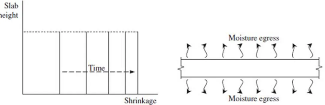
In the case of a simply supported beam, shrinkage deflection was evaluated considering the beam bent equally at the edges. Shrinkage deformation was considered uniform through the concrete depth as shown in figure 1.11:

(28)

26 Analytical models able to predict the long term behaviour of composite structure were proposed in the late of 80s. They are based on full-shear interaction theory and perfect bond between concrete and metal sheeting (Ghali, Favre, 1986; Gilbert, 1988). Ghali and Favre studied a composite prestressed beam and its time-dependent stress and strain. In the analysis, composite cross section were replaced by transformed section in which steel area were multiplied α times. The coefficient α is the ratio between young modulus of steel and young modulus of concrete. Young modulus of concrete varies considering creep and aging. The gradual development of creep and shrinkage increase the curvature on a generic cross-section of the beam. As a consequence, the beam deflection increases with time.

Gilbert (Gilbert, 1988) proposed to apply the Rate of Creep Method (RCM) to composite structures. The RCM is based on the assumption that the rate of change of creep with time is independent of the age of loading.

A single creep curve could be used for calculating creep strains to any stress history. This could cause an underestimation of creep in old concrete.

These approaches were adopted later to describe composite slabs behaviour, considering uniform shrinkage (UY, 1997; Koukkari, 1999).

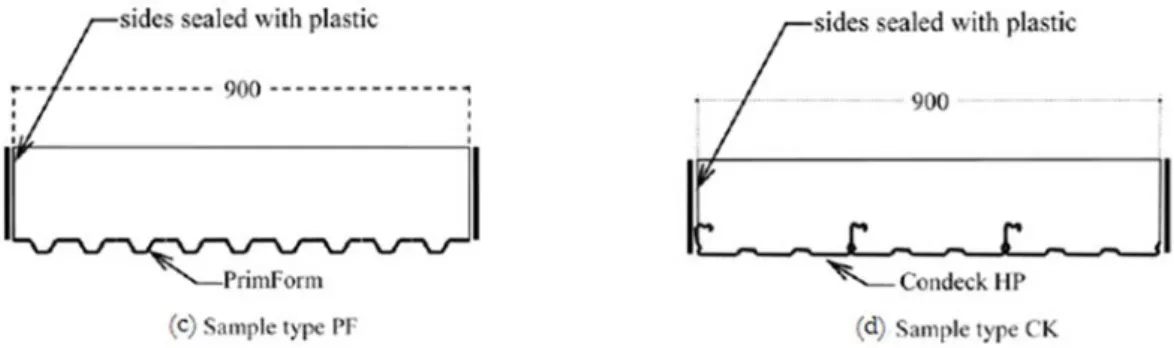
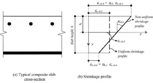
Recent studies (Ranzi, Vrcelj, 2009; Bradford, 2010; Al-Deen, 2011; Gilbert, Bradford, Gholamhoseini, Chang, 2011; Ranzi, Leoni, Zandonini, 2012; Al-deen, Ranzi, 2015) have demonstrated the presence of non-uniform shrinkage along a generic cross section. This is due to the presence of the sheeting, which results in a restraint to shrinkage and it prevents moisture’s egress from the soffit of composite slab. Experimental tests were performed on slabs in order to quantify non-uniform shrinkage deformations. Generally, a set of specimens were prepared and subdivided in samples free to dry on the bottom faces, samples sealed on the bottom faces by plastic layers and samples with the metal sheeting (figure 1.12). Every single specimen

(29)

27 is sealed on the lateral sides in order to eliminate drying in that direction and simulating the continuity of the slab as in a real floor structure.

Fig 1.12 Typical shrinkage profile specimens. (Gilbert, Bradford, Gholamhoseini, Chang, 2011)

Long-term deformations are monitored using strain gauges placed on the external surfaces and embedded on the concrete. Sealed and composite samples shows different strain readings through the depth with a higher shortening on the exposed face.

Bottom surface still exhibits non null deformation due to drying shrinkage. This was demonstrated by the presence of significant strain after 1 month of drying, which can’t be provided by autogenous shrinkage, because it tends to occur in the first two or three weeks after casting (Gilbert, Bradford, Gholamhoseini, Chang, 2011).

The total strains value on the top surface of the sealed samples could be 20-30% greater than those of samples free to dry on the bottom (Al-deen, Ranzi, 2015). Comparing the strain distribution in sealed and composite slabs, it can be shown the tensile restraining due to the presence of the steel sheeting, which reduces negative strains on bottom and increases them on top.

The thickness of the slab doesn’t influence this behaviour, even though deformations due to drying declines with lower value of the ratio of concrete surface to concrete volume.

(30)

28

Fig 1.13 Qualitative uniform shrinkage distribution for slab exposed on both sides (Ranzi, Leoni, Zandonini, 2012)

A simplified approach, for taking into account non-uniform shrinkage, was proposed (Al-deen, Ranzi, 2015) . It is based on a linear shrinkage profile, which allows to use uniform shrinkage deformation (figure 1.13) of the reinforced concrete slabs as reference.

The linear assumption (figure 1.14) is the simplest solution for the non-uniform shrinkage description and it is acceptable for design purpose: the uniform shrinkage deformation value, available on codes, is multiplied by coefficients, determined from experimental data, in order to define top and bottom strains of the slab.

Usually the coefficient for the top ranges between 1.1 and 1.2, while the value for the bottom is 0.2-0.3.

In this way the shrinkage profile is defined by a shrinkage strain at the level of the reference axis on the cross section and a shrinkage curvature.

In reality more complex profiles are present through the concrete thickness (Al-deen, Ranzi, 2015), so more refined functions could be used even if they aren’t convenient for the design.

(31)

29

Fig 1.14 Qualitative linear shrinkage distribution for composite slab. (Ranzi, Leoni, Zandonini, 2012)

Analytical formulations in (Bradford, 2010; Ranzi, Vrcelj, 2009) and numerical approach in (Al-deen, Ranzi, 2015; Gilbert, Bradford, Gholamhoseini, Chang, 2011) were proposed only recently in order to take into account the presence of non-uniform shrinkage on the cross-section analysis.

Bradford (Bradford, 2010) proposed a generic model for composite slabs subjected to concrete creep, concrete shrinkage and thermal strains; the method is based on principle of virtual work and a partial shear interaction theory.

Gilbert at al. (Gilbert, Bradford, Gholamhoseini, Chang, 2011) presented a numerical approach extending a long-term formulation described in (Gilbert, Ranzi, 2010) and based on the age-adjusted effective modulus method. Al-Deen and Ranzi (Al-deen, Ranzi, 2015) presented comparisons between calculated deflections using a simplified approach and experimental results available in literature.

(32)

30

2 Materials

2.1 Introduction

This chapter presents the material properties of the components of a composite steel-concrete slab. In the first part of the chapter the time dependent behaviour of steel-concrete is described, followed by the numerical methods that have been used to model it. The model used to take into account non-uniform shrinkage in composite slabs are then described. The material properties and constitutive laws of steel reinforcement and steel sheeting are presented in the last paragraph of the Chapter.

2.2 Concrete

2.2.1 Time Dependent Deformation of concrete

The time-dependent response may be defined as the long-term deformation it undergoes due to delayed strains arising from two phenomena, creep and shrinkage. Concrete creep strain develops over time due to a sustained stress. Conversely, shrinkage strain is completely independent of stress and only depends on the characteristic of particular concrete mix. At service load, this time-dependent inelastic effect may cause issues associated with increased deformation and curvature, and cracking in cases where shrinkage of concrete is restrained. This leads to problems with serviceability and durability of the system. It is possible to assume that the deformation of an uniaxially-loaded concrete specimen is the sum of three different components independent to each other (figure 2.1): the elastic strain εe(t), creep strain

εcr(t) and shrinkage strain εsh(t). The three components could be calculated separately

and summed up to obtain the total strain on concrete εc(t) as follows:

(33)

31

Fig 2.1 Concrete strain components (Gilbert, Ranzi, 2010)

2.2.2 The elastic deformation of concrete

The instantaneous strain occurs immediately after the application of the stress. A suitable constitutive model behaviour is required for the prediction of the instantaneous behaviour of concrete.

When concrete is subjected to compression, it is assumed to remain in its linear-elastic range. If concrete is in tension, the behaviour can be even considered linearly elastic until reaching the tensile capacity. The concrete is expected to crack in tension once it reaches its tensile strength.

For element in flexure, the characteristic flexural tensile strength , of concrete has

been assumed as a tensile capacity.

The linear-elastic uniaxial model consists of Hooke’s Law and can be written as follows:

(2.2) where is the time of loading.

2.2.3 Creep

Creep originates in the hardened cement paste while aggregates provide only restraint to the deformation. The cement paste consists of a rigid cement gel with many

(34)

32 capillary, which is made of colloidal sheets formed by calcium silicate hydrates and evaporable water. The mechanism through which creep occurs is causes of controversies among the scientific community and at present there is no satisfactory theory available to describe the formation of creep. Bazant suggested that creep is due to the disorder and instability that characterize the bond between the colloidal sheets. (Bazant, 1972)

Many factors influence the magnitude and the rate of development of creep. These factors are generally categorized in two different groups: the technological parameters and the external parameters. The technological parameters are associated the concrete mix (water/cement ratio, type of aggregates, mechanical properties and type of cement). In general, an increase in either the aggregate content or the maximum aggregate size reduces creep. The same happens with the use of a stiffer aggregate. Creep decreases also with lower water-to-cement ratio. The second group of parameters are the one associated with the ambient conditions, the geometry of the element and the loading conditions. Creep increases as the relative humidity decreases and it is also greater in members with large surface-area-to-volume ratios, such as slabs. It is also dependent on the ambient temperature. Higher temperature increases the deformability of the cement paste and accelerates drying. This accelerates creep. In addition, creep depends on the loading history, e.g. the magnitude and duration of the stress and the age of concrete when the stress is first applied. It shows a marked aging effect: older concrete creeps less than concrete loaded at early ages, even if creep never totally disappears. If the concrete stress is less than about 0.5fc’, creep is approximately

proportional to the stress and is known as linear creep. At higher level of stress creep

increases non-linearly with respect to stress. This behaviour is thought to be related to an increase of micro cracking.

In general creep increases over time until the load is maintained, tending to an asymptotic value (which can be equal to 3-4 times the initial elastic deformation). Its rate of increase slows down with time. If the load is removed, it can be observed an instantaneous recovery of the elastic deformation and a gradual reduction of part of creep over time. Creep is significantly greater when accompanied by shrinkage. The

(35)

33 additional creep due to drying is known as drying creep. If the specimen is in hygral equilibrium with the environment, the time dependent deformation due to the stress is referred as basic creep.

2.2.4 Shrinkage

Shrinkage may be defined as the change in concrete volume over time. The strain is independent of stress. Shrinkage can be of different types: plastic shrinkage, chemicals shrinkage, thermal shrinkage and drying shrinkage.

The plastic shrinkage is a contraction the concrete volume undergoes when is still in the plastic phase. The plastic shrinkage affects mostly on horizontal surface exposed to the air, which is therefore exposed to the risk of cracking: it tends to contract, but is opposed by the core below that does not shrink; the cortical zone enters then in traction. If the traction exceeds the (very low) tensile strength of the concrete in phase plastic, cracks will appear. At this stage the bond between the plastic concrete and the reinforcement has not yet developed, so the steel can’t control cracks. Plastic shrinkage can be avoided while maintaining the jet in an environment saturated with steam, for example through the use of anti-evaporating membranes.

Chemical shrinkage (also called autogenous shrinkage) is a contraction of the concrete volume undergoes after hardening, even when it is maintained at a constant temperature and prevents any possible moisture exchange with the external environment. It is associated to chemical reactions, i.e. the hydration reaction of cement. The effects of autogenous shrinkage are exhausted in the first days after casting and are usually not noticeable in ordinary concrete. Instead, in high performance concrete, which mixture is characterized by a low ratio water / cement, the effects of autogenous shrinkage are well more than appreciable and may even cause the cracking of the elements if prevented by internal or external constraints (Tazawa , Miyazawa , 1992).

In ordinary structures made of concrete with low water/cement ratio, the effects of autogenous shrinkage can be mitigated by careful and prolonged curing of the surfaces to air.

(36)

34 If the concrete is located in an environment with not saturated humidity (RH <95%) tends to dry out and shrink. This effect is known as drying shrinkage, and can affect the hardened concrete of any age, as long as this is exposed to an environment with U.R. less than 95%. It increases in time with decreasing rate.

Thermal shrinkage is the contraction due to the dissipation of heat coming from hydration. It results in the first few hours after casting.

(37)

35

2.3 Numerical methods for time analysis of concrete

2.3.1 The superposition integral

The time dependent behaviour of concrete is described by means of the superposition integral which is defined based on the guideline proposed in (CEB, 1984) as follows:

1 ,

,

(2.3) Where t is the time from casting, τ is the time of loading, τ0 is the time of first loading,

σc is the concrete axial stress, φ(t, τ) is the creep coefficient and J(t, τ) is the creep

function. The creep coefficient is defined as the strain at time t caused by a constant

unit stress first applied at age τ. It can be expressed as follows:

, ,

(2.4)

Summing the instantaneous and creep strains due to an unitary stress, the creep function J(t,τ) is obtained as follows:

, 1 1 ,

(2.5) Numerical values of φ(t, τ) and εsh(t) are available in standard codes. In this work

thesis, the Australian standard code for concrete structures (AS3600, 2009) has been used. The formulation is outlined in Appendix 1.

The superposition integral is based on the principle of superposition. The principle of superposition was applied first to concrete by McHenry (McHenry, 1943). It stated

(38)

36 that strain produced by a stress increment applied at any time τ is not affected by any stress applied either earlier or later.

Since the superposition integral cannot be solved in closed form, numerical solutions of the integral are necessary.

2.3.2 The effective modulus method (EMM)

The instantaneous and creep components of strain were combined and an effective modulus for concrete Eef(t,τ0) was defined. In the EMM, equation 2.3 is approximated

by assuming that the stress-dependent deformations are produced only by a sustained stress equal to the final value of the stress history at time t. The formulation is outlined

in the following:

, 1 ,

(2.6) Where the effective modulus has been defined as follows:

,

1 ,

(2.7) Creep is treated as a delayed elastic strain and it is taken into account simply reducing the elastic modulus of concrete with time.

The ageing of the concrete has been ignored.

2.3.3 The age-adjusted effective modulus method (AEMM)

A simple adjustment of the effective modulus method to account the ageing of concrete was proposed by Trost (Trost, 1967). Later the method was more rigorously

(39)

37 formulated and further developed by Dilger and Nevile (Dilger, Neville, 1971) and Bazant (Bazant, 1972).

A reduced creep coefficient can be used to calculate creep strain if stress is gradually applied. The reduced creep coefficient is χ(t,τ0)φ(t, τ), where the coefficient χ(t,τ0) is

called the ageing coefficient.

Using the AEMM the total strain at time t can be expressed as the sum of the strains

produced by σc(τ0)(instanteneous and creep), and the strains produced by a gradually

applied stress increment Δσc(t).

The concrete strain at time t can be expressed as follows:

0

,

(2.8) where Eef(t,τ0) is the effective modulus method of equation 2.7 and ef(t,τ0) is the age

adjusted effective modulus given by:

,

1 , ,

(2.9) With the AEMM, two analyses need to be carried out: one at first loading (time τ0) and

(40)

38

2.3.4 The Step-by-step method (SSM)

Considering the stress history in figure 2.2, the time under load could be divided into

n steps. The continuously time-stress curve could be approximated by a series of small

stress increments.

Fig 2.2 Time-stress history (Gilbert, Ranzi, 2010)

The actual stress history is approximated by a step-wise variation of stress. In this simplification, the period of sustained stress is divided into k time intervals with the

age at first loading designated and the end of the period of sustained stress designated (figure 2.3).

Fig 2.3 Time discretization (Gilbert, Ranzi, 2010)

The time discretization used in this thesis work, based on a geometrical progression, is the following:

(41)

39 (2.10) where is the period in which sustained stress is present, k is the total number of time intervals and j is the time interval considered.

The total concrete strain at the end of the time period may be approximated by:

, , ∆

(2.11) where:

, is the creep (compliance) function calculated at time related to a unit stress applied at time .

∆ is calculated as and represents the stress variation that occurs between times and . The simplification introduced by the step-by-step method is that the stress is assumed to remain constant during each time interval and so for a more accurate prediction is needed a big number of time intervals. The bigger this number, the higher is the computational difficulty.

The time discretization should be such that an approximately equal portion of the creep coefficient , develops during each time step (Gilbert, Ranzi, 2010). In this thesis, the equation approximates the integral-type creep law by means of the so-called rectangular rule.

Simplifying the notation, the equation (2.11) becomes:

, , , ∆ , ,

(42)

40 Rearranging the equation (2.12):

, , , ,∆ , , , , , , , , , , , , , , , , , , , , , , , , , , , , , , , , , , , , , , , , , , , , , , , , , , , , , , , (2.13a-g) The equation (2.13g) can be arranged in terms of stress and the constitutive relationship for the concrete becomes:

, ,

,

, ,

, , , , , , ,

(2.14)

(43)

41

,

1

,

(2.15) And , ,is the stress modification factor:

, , , ,

,

(2.16) For each time step, , and , , must be specified and the previous stress history

must be stored throughout the analysis.

However, the SSM is not subject to many of the simplifying assumptions contained in other methods of analysis and generally leads to reliable results. For most practical problems, satisfactory results are obtained using as few as 6–10 time intervals (Gilbert, Ranzi, 2010).

(44)

42

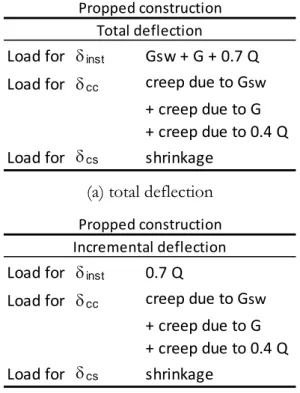
2.4 The non-uniform shrinkage on composite slab cross-section

If drying occurs at different rate from the top and bottom surfaces, the total strain distribution is no longer uniform over the depth of the section.

As previously discussed, recent studies (Ranzi, Vrcelj, 2009; Bradford, 2010; Al-Deen, 2011; Gilbert, Bradford, Gholamhoseini, Chang, 2011; Ranzi, Leoni, Zandonini, 2012; Al-deen, Ranzi, 2015b) have demonstrated the occurrence of non-uniform shrinkage on composite slab cross-section (as shown in figure 2.4 and figure 2.5).

Fig 2.4 Composite samples for shrinkage measurement (Al-Deen, Ranzi, 2015b)

Fig 2.5 Total long-term measured at different instances in time through the cross-section

In current design guidelines, the non-uniform free shrinkage distribution is not present. The simplest possible profile to model non-uniform shrinkage is a linear distribution, even though more complex shrinkage profiles occur through the thickness. For this purpose Al-Deen and Ranzi (Al-deen, Ranzi, 2015b) proposed a linear shrinkage distribution based on the free shrinkage for conventional concrete slabs. This distribution is available from codes or measured experimentally.

(45)

43 The non-uniform free shrinkage profile for composite slabs can be described by the top and bottom strain:

, , , ,

(2.17) where subscript indices k refers to the time instant in which strains are computed. ,

is the free shrinkage distribution of a slab exposed on both sides.

The coefficients , and , are determined experimentally in the study (Al-deen,

Ranzi, 2015b). For routine design it has been recommended to set this coefficient as follows:

, 1.2

, 0.2

(2.18) The shrinkage profile could be also express by the shrinkage strain measured at the level of the cross-section reference axis, , , and an additional curvature , , .

, , , , ,

(2.19) In which is the position of the reference axis with respect of top (figure 2.6).

(46)

44

Fig 2.6 Strain variables describing non-uniform free shrinkage on composite slabs

2.4.1 Comparison with experimental results

A sectional analysis using the linear shrinkage profile, above introduced, has been used for the calculation of a slab deflection in (Al-deen, Ranzi, 2015b), where the behavior of concrete was modeled using the age-adjusted effective modulus method. The results were compared with the experimental results of samples described in (Al-deen, Ranzi, Uy, 2015; Ranzi, Al-Deen, Ambrogi, Uy, 2013). It turned out that, when the linear shrinkage profile is assumed, the calculation predicted the long-term deflections of the slabs with acceptable accuracy. The study highlighted also that the use of uniform shrinkage profiles leads to underestimation of the deflections.

Another validation has been done using experimental results achieved at the Laboratory of the School of Civil and Environmental Engineering - The University of New South Wales (Gholamhoseini, 2014). The experimental program involved the testing of ten simple-span composite slabs under different sustained, uniformly distributed load for periods up to 240 days. In particular, the validation considered four out of ten slabs, which are identified by the codes 1LT-70-0, 2LT-70-3, 3LT-70-3 and 4LT-70-6. The four slabs have the same metal sheeting profile.

(47)

45 The centre to centre distance between the two end supports was 3100 mm. The slabs were subjected to different levels of sustained loading, which has been applied at age 64 days.

Slab 1LT-70-0 carried only the self-weight for the full test duration, slabs 2LT-70-3 and 3LT-70-3 were identical and carried a constant superimposed sustained load of 3.4 kPa and slab 4LT-70-6 carried a sustained load of 6 kPa.

The results of the comparisons between experimental long-term deflection and the computed long-term deflection are outlined in table 2-1.

Note: deflection in mm

Table 2-1 Validation of the linear shrinkage

The results highlight the linear shrinkage profile assumption well represents the long term behaviour of composite slab. It is worth to notice the computation of deflections has been performed by means of a cross-sectional analysis, which is a relatively simple approach suitable for practical applications.

CALCULATED RATIO 1LT‐70‐0 4.04 3.76 0.93 2LT‐70‐3 6.72 6.22 1.08 3LT‐70‐4 5.84 6.22 0.94 4LT‐70‐6 6.4 8.50 0.75 TEST LINEAR SHRINKAGE SLAB 247 days

(48)

46

2.5 Steel

2.5.1 Conventional, non-prestressed reinforcement

With regard to serviceability, steel reinforcement can be useful to reduce both immediate and time-dependent deformations. Adequate quantities of bonded, non-prestressed steel also provide crack control.

In Australia, reinforcing bars are two types, Grade R250N and Grade D500N (250 and 500 refers to the characteristic yield stresses of 250 MPa and 500 MPa, respectively). Grade R250N bars are hot-rolled plain round bars of 6 or 10 mm diameter (designated R6 and R10 bars) and are commonly used for fitments such as ties and stirrups. Grade D500N bars are hot-rolled deformed bars with sizes ranging from 12 to 40 mm diameter (in 4 mm increments).

In design calculations, the constitutive law of steel is usually considered to be elastic- perfectly plastic. In the elastic range, steel stress is proportional to the steel strain

:

Where is the elastic modulus of the steel. After yielding the stress–strain curve was assumed to be horizontal (perfectly plastic), ignoring the hardening. The stress-strain curve in compression is equal to that in tension. At service loads, the stress in the non-prestressed steel is usually less than the yield stress and behaviour is linear-elastic.

(49)

47

2.5.2 Metal Sheeting

In many cases, the deflection under fresh concrete is the parameter governing the sheet selection. The steel sheeting has to support not only concrete weight during hardening, but also the heaping of concrete and the pumping loads.

Fig 2.7 The metal sheeting

The sheeting thickness ranges between 0.6 mm and 1.2 mm. It is very thin for economic reasons. Typically, they are 1 m wide and up to 6 m long and they are designed to span only in one direction. The sheets are usually pressed or cold-formed and are galvanized to resist corrosion,

The nominal yield strength is that of the flat sheet from which the element is made. Now, products are available with a yielding stress equal to 550 MPa. The elastic modulus is 200000 MPa.

The considered constitutive law is assumed elastic-perfectly plastic as ordinary reinforcement steel (figure 2.8).

(50)

48 In this thesis, two different profiles have been considered, which are referred to as profile 1 and profile 2 (figure 2.9). The geometric properties are summarized in table 2-2.

Table 2-2 Geometric properties of the profiled steel sheeting

Where tms is the thickness of the profile. Ams is the area per unit width of the profile,

yms is the centroid of the metal sheeting with respect to the bottom flange, Ims is the

inertia per unit width.

(a) Profile 1 (b) Profile 2

Fig 2.9 Geometry of the profiled steel sheeting

Profile tms Ams yms Ims Mass

[.] [mm] [mm2/m] [mm] [mm4/m] [kg/m2]

1 1 1678 15.50 445050 13.79

(51)

49

3 Design of composite slab

3.1 Introduction

This chapter describes the ultimate and service limit state design of simply-supported composite steel-concrete slabs based on the Australian design rules as reference. In particular, the proposed formulation is based on the new Australian draft code for composite steel-composite structures (AS2327 Draft, 2015). The ultimate limit state design rules specified in this code are similar to those recommended in the European guidelines (EN 1994-1.1, 2004) and are presented in the first part of the chapter, followed by the description of the serviceability requirements. The Australian approach differs from current international guidelines for the attention placed at considering a concrete shrinkage gradient, which develops dues to the inability of the concrete to dry from its underside, for the serviceability limit state requirements. In particular, this non-uniform shrinkage profile has been accounted for with a linear distribution as presented in chapter 2. Other international guidelines enable, within specified range of span to-depth-ratio, to omit deflection calculations and, when not satisfying these requirements, permit to carry out the service slab design without considering the occurrence of shrinkage. When shrinkage effects are considered, the design is based on a uniform shrinkage profile.

In the second part of the chapter, an extensive parametric study is carried out considering the design of composite slabs carried out based on the three serviceability models, i.e. the first model accounting for the shrinkage gradient, the second approach relying on a constant (uniform) shrinkage profile and the third procedure ignoring shrinkage effects. The numerical calculations and design have been implemented in a Matlab program. The main aims of the parametric study are to evaluate the differences produced by the three serviceability procedures on the composite slabs’ design for different loading conditions, cross-sectional properties and floor arrangements.

(52)

50

3.2 Limit state requirements specified by Australian draft code AS2327

3.2.1 Ultimate limit state: Flexure

The draft code states that the bending resistance MRd shall be determined by plastic

theory based on full or partial shear connection and that the partial shear connection method can be used for slabs with a ductile longitudinal shear behaviour.

The design bending moment shall not exceed the design resistance MRd which is:

, ,

(3.1) where:

, = design axial force resisted by the profiled sheeting

, = plastic resistance moment of the profiled steel sheeting reduced by

the axial force , . Its value can be taken equal to:

1.25 , 1 ,

, ,

, = design plastic resistance in bending of the profiled sheeting

= capacity reduction factor

= nominal plastic resistance in bending of profiled sheeting = composite level arm calculated with equation (3.2)

The design axial load force resisted by the profiled sheeting , at a particular

cross-section is:

, = min( , , ,

where:

, is the design axial force resisted by the profiled sheeting in full shear connection

(53)

51

, min , , ,

in which:

, design axial force resisted by the profiled sheeting at yield

_,

,

′

capacity reduction factor and

, design axial force resisted by the shear connection between the profiled

sheeting and the concrete slab relying on the mechanical or frictional interlock ,

, design shear strength obtained from slab test meeting the basic

requirements of the partial connection method.

distance of the cross-section being considered to the nearest support for a simply supported slab

At a particular cross-section, the design is classified as based on full or partial shear connection depending on the magnitude of the axial force resisted by the profiled sheeting:

full shear connection if , ,

partial shear connection if , < ,

For simplification, the distance z shall be determined based on:

0.5 ,

,

(3.2) where:

(54)

52 the section is designed in full shear connection with (i.e. if the neutral axis is above the steel sheeting as shown in figure 3.1); or

when the section is designed in full shear connection and (i.e. if the neutral axis is in the steel sheeting as shown in figure 3.2).

location of the plastic neutral axis from the extreme compressive fibre of the composite slab

, / 0.85

e distance from the centroidal axis of the profiled sheeting to the extreme fibre of the composite slab in tension

distance from the plastic neutral axis of the profiled sheeting to the extreme fibre of the composite slab in tension

Figures 3.1 and 3.2 show the stress distribution on the cross-section if the neutral axis is above and below the steel sheeting respectively:

Fig 3.1 Stress distribution for sagging bending if the neutral axis is above the steel sheeting (Draft AS2327)

(55)

53

3.2.2 Ultimate limit state: Vertical shear

A composite steel concrete slab can be considered as a beam without shear reinforcement. The vertical shear resistance can be determined in accordance with the Australian standard code for concrete structures (AS3600, 2009)as follows:

/

where:

= / 4

=

= 1.1 1.6 /1000 0.8 = 1 (if no axial action is considered) = 1 (if only gravity loadings are presented)

= the distance from the extreme compression fibre of the concrete to the centroid of the outermost layer of tensile reinforcement

= the area of the longitudinal steel provided in the tensile zone (the metal sheet for composite slab)

= minimum effective web width in mm (the width for composite slab)

3.2.3 Serviceability limit state: deflection

The calculated defection should not exceed the deflection limits that are appropriate to the structure and its intended use. The deflection limits are expressed in terms of deflection-to-span ratio and are applied to both total deflection and incremental deflection.

The total deflection is the final long-term deflection of the slab that is calculated as the sum of the short-term and time-dependent deflection caused by the dead load (including self-weight), the expected in service live load and the effects of shrinkage. The limit on the incremental deflection is imposed to avoid damages on brittle partitions or floor finishes.

(56)

54 The incremental deflection is a portion of the total deflection that occurs after the attachment or installation of the non-structural elements that can be damaged. Total deflection and incremental deflection can be expressed as follows:

, , , (3.3 a,b) where: = instantaneous deflection = creep deflection = shrinkage deflection

and the subscript incr refers to the incremental deflection.

The loads resisted by the composite floor system for the purpose of the deflection calculations vary depend on the adopted construction procedure. In the case of unpropped construction, the self-weight of the wet concrete is carried by the steel sheeting which acts as permanent formwork, while all loads applied after the removal of the props are resisted by the composite action. In the case of propped construction, the composite member resists all applied loads, including its self-weight.

The total and incremental deflections are usually calculated and measured from the top of the concrete slab, unless particular aesthetics requirements are specified for the underside of the floor.

The service load combinations adopted for propped and unpropped construction are summarized in tables 3-1 and tables 3-2, respectively. The static configuration of the slab is shown in figure 3.3.

(57)

55 (a) total deflection

(b) incremental deflection

Table 3-1 Load combinations for the evaluation of deflections in propped construction

(a) total deflection

(b) incremental deflection

Table 3-2 Load combinations for the evaluation of deflections in unpropped construction

Load for inst Gsw + G + 0.7 Q Load for cc creep due to Gsw + creep due to G + creep due to 0.4 Q Load for cs shrinkage Propped construction Total deflection Load for inst 0.7 Q Load for cc creep due to Gsw + creep due to G + creep due to 0.4 Q Load for cs shrinkage Propped construction Incremental deflection Load for inst G + 0.7 Q Load for cc creep due to G + creep due to 0.4 Q Load for cs shrinkage Unpropped construction Total deflection Load for inst 0.7 Q Load for cc creep due to G + creep due to 0.4 Q Load for cs shrinkage Unpropped construction Incremental deflection