Citizen science as a tool for the environmental quality assessment of the Mediterranean coastal habitats

UNIVERSITÀ DI BOLOGNA

SCUOLA DI SCIENZE

Corso di laurea magistrale in BIOLOGIA MARINA

Citizen science as a tool for the environmental quality

assessment of Mediterranean coastal habitats

Tesi di laurea in Habitat marini rischi e tutela

Relatore

Presentata da

Prof. Marco Abbiati

Eva Turicchia

Correlatori

Dott. Massimo Ponti

Prof. Carlo Cerrano

Table of contents

1

Introduction ... 3

1.1 Environmental quality assessment and the need of reliable indices 3 1.1.1 Types of indices ... 3

1.1.2 Review of indices available for the Mediterranean marine habitats ... 4

1.2 Thematic maps ... 6

1.2.1 Territorial units and administrative boundaries ... 6

1.2.2 Species distribution and habitats mapping ... 7

1.2.3 Maps of natural emergencies ... 7

1.2.4 Environmental degradation and risk maps ... 7

1.2.5 Vulnerability maps ... 8

1.2.6 Environmental and ecological quality maps ... 8

1.2.7 Susceptibility to use map ... 8

1.3 Citizen science: an essential contribution ... 9

1.3.1 Development of indices based on data collected by volunteers ... 10

1.4 Aims of the study ... 11

2

Material and methods ... 13

2.1 The Reef Check Italia onlus protocol ... 13

2.1.1 Visual census method and participant training ... 13

2.1.2 Data mining and validation ... 16

2.1.3 Volunteers data survey validation ... 17

2.2 Territorial units and temporal periods ... 17

2.3 Development of indices ... 19

2.3.1 Species diversity indices ... 19

2.3.2 Non-indigenous species indices ... 22

2.3.3 Species sensitive assessment ... 23

3.1 Reliability of data collected by RCI volunteers ... 32

3.2 RCI database contents ... 33

3.3 Mediterranean Reef Check Diversity indices ... 38

3.3.1 Mediterranean Reef Check Species richness ratio index... 38

3.3.2 Mediterranean Reef Check Species diversity index ... 39

3.3.3 Mediterranean Reef Check Species heterogeneity index ... 41

3.4 Mediterranean Reef Check NIS indices ... 43

3.4.1 Caulerpa cylindracea ... 44

3.4.2 Caulerpa taxifolia ... 46

3.4.3 Rapana venosa ... 48

3.5 Mediterranean Reef Check Species sensitive indices ... 50

3.5.1 MRC-Ss indices applied to Marine Protected Areas ... 53

3.5.2 Effectiveness of the MRC-Ss indices ... 54

4

Discussion ... 57

1

Introduction

1.1

Environmental quality assessment and the need of reliable

indices

The human impacts on the ecosystems and living resources have grown in the last century. Coastal areas are among the most threatened marine environment and the need of environmental quality assessment tools is urgent (Rosenberg et al. 2004). This can be obtained by developing and applying reliable biotic indices, which may provide complementary information on marine community and support decision-making processes.

1.1.1 Types of indices

Different types of indices have been used in ecology for environmental quality assessment ranging from species diversity to biotic indices, from single metric to multimetric indices.

Species diversity indices are focused on the trade-off between diversity and disturbance: as a classic paradigm, normally the diversity increase when the disturbance decreases (e.g. Rosenberg et al. 2001). Measures of local species diversity (α-diversity; sensu Whittaker 1972) may focus on the number of living specie (species richness), on the relative dominance in terms of individual abundance (evenness, e.g. Pielou and Simpson indices) or on the combination of these two components (e.g. Shannon index; Magurran 2004). A biotic index is a measure for rating the environmental quality based on biological and ecological attributes of the organism living in the study site. It should provide quantitative information on ecological condition, structure and functioning of ecosystems (Jørgensen et al. 2005, Ponti et al. 2009). The multimetric approach provides an integrate analysis by combining different categories of metrics which reflect

1.1.2 Review of indices available for the Mediterranean marine habitats

According to the current European legislation, the achievement and maintaining good status for marine coastal water are compulsory goals for the European national governments. Through the enforcement of the Water Framework Directive (WFD; Directive 2000/60/EC) and the Marine Strategy Framework Directive (MSFD; Directive 2008/56/EC), the European Union encourages the conservation of aquatic systems and the development of management strategies for water resources. Thus, tools to assess the ecological quality status of marine environment are mandatory for achieving the settled goals and adopting strategies to preserve the water quality from worsening. With these aims, several studies were focused on the identification of biological indicators and biotic indices able to assess the ecological water quality of marine ecosystem (Casazza et al. 2002, Borja et al. 2004, Simboura et al. 2005, Borja et al. 2009, Leonardsson et al. 2009, Van Hoey et al. 2010). Some of the proposed ecological indices take into account the presence/absence of a given indicator species, while others are focused on the species diversity, the different ecological strategies adopted by organisms, or finally the energy variation in the system as a results of a changes in the biomass of specimens (Salas et al. 2006).

Among the indices developed to assess the environmental quality of Mediterranean habitats, there are: the CARtographic of LITtoral rocky shore communities (CARLIT), which is based on the occurrence of macroalgae communities (Ballesteros et al. 2007a, Ballesteros et al. 2007b, Mangialajo et al. 2007, Asnaghi et al. 2009); the Ecological Evaluation Index (EEI), for subtidal coastal and transitional waters, focusing on the morpho-fuctional characteristic of the most common macroalgae and their growth strategy (Orfanidis et al. 2011); and the Ecosystem-Based Quality Index (EBQI) dedicated to assess the functioning of the posidonia meadows (Personnic et al. 2014). Review of the indices developed for the Mediterranean coastal lagoons can be found in

Reef Scape Estimate index (COARSE; Gatti et al. 2012, Gatti et al. 2015) and the Ecological Status of Coralligenous Assemblages (ESCA; Cecchi et al. 2014). The CAI is a multimetric index based on percent cover of bryozoans, sludge and builder species (Deter et al. 2012).

The purpose of CAI is to evaluate the water quality on the base of coralligenous assemblages. Coralligenous assemblages were analysed using two non-destructive protocols: photographic quadrats and demography of erected species. The sample sites were chosen to represent different human pressure. The metrics were selected through a linear regression based on a different index (Anthropogenic

Pressure Index) that includes three descriptors of water quality according to

thresholds set by the Agency for French waters. The reference conditions were defined as the best result among the selected metrics for the index. The index was developed using one-year data in one area, therefore it need for more validation. COARSE multimetric index integrates biological, ecological and geomorphologic information obtained using a Rapid Visual Assessment technique, which appear very subjective, with metrics of doubtful utility and a limited replication. Furthermore, the construction and validation was done without using independent dataset.

The ESCA multimetric index is mainly based on the macroalgae assemblages (Cecchi et al. 2014). The index was developed based on previous impact evaluation studies on the NIS Caulerpa cylindracea, the increasing rate of sedimentation and the nutrient enrichment. It was validated on an independent dataset collected during a 3-year study carried out at five sites in the Tyrrhenian Sea, and tested on a gradient of anthropogenic stressors. Assemblage descriptors selected as metrics were: presence/absence and abundance of sensitive taxa/groups, α-diversity and β-diversity of assemblages.

On overall, the proposed indices for coralligenous habitats still seem unreliable, approximate, little based on ecological and functional, and lacking in a rigorous definition of the reference conditions.

1.2

Thematic maps

The Mediterranean Sea is a global biodiversity hot spot challenged by increasing human pressure, which includes pollution, habitat modification, harvesting and climate change (Worm et al. 2006, Jackson 2008, Micheli et al. 2013). The implementation of efficient management tools, such as thematic maps, are needed to ensure long-term ecosystem conservation and the availability of goods and services they provide (Palumbi et al. 2009, Curtin & Prellezo 2010, Katsanevakis et al. 2011, Craig 2012, Ostendorf 2011, Bierman et al. 2011).

The Integrated Coastal Zone Management (ICZM) and the Ecosystem Based Management (EBM) are integrated approaches that consider the entire ecosystem, including humans. It provides a mechanism for a strategic and integrated plan-based approach for marine management. Given the territorial nature of EBM, the diagnostic cartography is the tool needed for its application (Curtin & Prellezo 2010, Katsanevakis et al. 2011, Bianchi et al. 2012, Meidinger et al. 2013). Through the application of suitable indicator and indices, diagnostic cartography describes, links and visually represents the relationship between human impacts and the status of coastal and marine ecosystem.

1.2.1 Territorial units and administrative boundaries

Thematic maps are designed to communicate quantitative and/ or qualitative data (attributes) related to defined areas. Areas are normally divided in small and manageable units, which are called territorial unit. Territorial units may coincide with administrative territories (e.g. municipalities, provinces, management and monitoring zones within a marine protected area), otherwise they could be defined according to environmental criteria (e.g. habitats) or ultimately they could be represented by grid cells of manageable size (Bianchi et al. 2012). The choice of suitable territorial unit depends on several considerations including the objective and purpose of spatial analysis, data organization, distribution and density of

1.2.2 Species distribution and habitats mapping

Along with the morpho-bathymetric and sedimentological maps, habitat and bionomic maps are among the most common cartographic tools used to characterise the marine environment. They provide the basis for subsequent spatial analyses (Bianchi et al. 2012, Meidinger et al. 2013). Bionomic maps are important to understand ecological processes occurring in marine habitats.

1.2.3 Maps of natural emergencies

A natural emergency is a natural feature, species or habitat, which requires intervention to prevent a status worsening. Therefore, natural emergencies may be represented by protected species and/or protected habitats according to national laws and international conventions. From a management point of view, protected species can be distinguished in three main categories: those in need of strict protection (e.g. Annex IV of the European Habitats Directive, 92/43/EEC); those requiring to be considered in the management actions (e.g. Annex V of the Habitats Directive); and those listed as endangered but no particular conservation measures are required (e.g. in the Annexes of the Washington Convention on the International Trade in Endangered Species of wild fauna and flora, CITES; Bianchi et al. 2012). By analogy, threatened habitats could be divided in priority

habitats, for which protection is mandatory (e.g. Posidonia oceanica meadow and

coastal lagoons in the Annex I of the Habitats Directive), and other sensitive habitats which should deserve more attention (e.g. the coralligenous and other calcareous bio-concretions in the Mediterranean Sea, UNEP-MAP-RAC/SPA 2008). Thus, a natural emergencies map provides synthetic information showing the level of attention and practical intervention that should be given to distinct areas of the marine territory. However, the information on the updated distribution of protected species are hardly available for mapping (Possingham et al. 2007).

A map describing the environmental degradation has to take into account the level, intensity and quality, of coastal urbanization and visualize indices/ indicators of marine ecosystem alterations (Borja et al. 2009, Bianchi et al. 2012, Coll et al. 2012). The levels of degradation could be represented by different colour. Each colour means a decrease in naturalness, hence an increase in environmental degradation. Specific symbols overlaid can inform on potential risks (infrastructures, pollution, urban and tourist development, fishery for examples) in the investigated area (Bianchi et al. 2012).

1.2.5 Vulnerability maps

The fragility or vulnerability to exogenous and endogenous stress factors is the capacity of the ecosystem of maintains its structure and functions when facing real or potential unfavourable influences. Vulnerability may be assigned at the habitat level (e.g. in Bellan-Santini et al. 2002) and can account for the rarity of each habitat in the area of interest (Bianchi et al. 2012).

1.2.6 Environmental and ecological quality maps

Measure and mapping the environmental and ecological quality is one of the most important steps in ICZM and EBM. According to Bianchi et al. (2012), the overall environmental quality may be assessed by combining the potential quality of the habitats (obtained, for instance, assigning a natural, economic, aesthetic, and rarity values to each habitat; Bardat et al. 1997) with the level of degradation or integrity (e.g. considering the physical, chemical and biological characteristics, as provided in the MSFD for the seafloors). In this respect, adequate indicators and indices, for instance based on sensitivity of species towards diverse sources of disturbance, may provide further insights in different habitats (Diaz et al. 2004, Rosenberg et al. 2004, Van Hoey et al. 2010).

relationship between the habitat importance according to law and the presence of protected species according to law as well. The result is an easy management tool to discriminate areas subordinated to conservation (strict protection) from areas where the conservation is not tightly required (maximum availability) (Bianchi et al. 2012).

1.3

Citizen science: an essential contribution

Citizen science (CS) is the involvement of non-technical volunteers as researchers. CS has grown up in the last decades and it has become more important in conservation science (Whitelaw et al. 2003, Conrad & Hilchey 2011). The growing factors are primarily the increasing awareness that volunteers are a free source of skills, labour-force and computational power and secondly the existence of informatics tools that can spread easily the information about project and gathering data from the participants (Silvertown 2009). However, there is scepticism about the reliability of the data collected by the volunteers since they are often lack of experience and knowledge. Especially, the data generated by volunteers’ surveys could contain great levels of bias or variability. The differences in skills among the volunteers would lead to decreased accuracy in measurements and misidentification of species. Actually, they are potentially a great scientific resource and not a means to acquire high quality data cheaply. The science has neither the manpower nor the financial resources and the time to cope with the demands that scientific research requires. The volunteers then become a large workforce and could contribute to applied research through their participation in monitoring programs in which experience scientists lead them. So the citizens could help scientists to collect broad-scale data thereby bridging the funds and time lack (Mumby et al. 1995, Dickinson et al. 2010, Zoellick et al. 2012, Tulloch et al. 2013, Bird et al. 2013, Whitelaw et al. 2003, Conrad & Hilchey 2011, Foster-Smith & Evans 2003, Holt et al. 2013).

enhance the ability of decision-makers, stakeholders and non-government organizations to monitor, manage and conserve natural resources, while citizen volunteers are increasingly involved in local issues and more awareness in environmental threats and careful about theirs everyday actions toward the environment (Alaback 2012, Conrad & Hilchey 2011, Whitelaw et al. 2003, Tulloch et al. 2013).

1.3.1 Development of indices based on data collected by volunteers

Citizen science provides a large amount of data about species occurrence and distribution around the world and over long spans of time. Several projects have used these data for descriptive statistics, developing indices and, on overall, for advancing scientific knowledge.

Over the past three decades, the growing of scuba diving activities has encouraged the broad involvement of recreational divers for marine monitoring. Two broadly successful citizen science programs are the ones developed by Reef Check Foundation (www.reefcheck.org; Hodgson 1999, Hodgson 2001, Hodgson et al. 2006), based in California and with several national agencies around the World, and Coral Watch non-profit organization (www.coralwatch.org), based in Australia. The aim of both is to integrate global reef monitoring with participants education. Coral Watch has recruited volunteers from more than 60 countries and its methodology has been applied in several published scientific papers (Leiper et al. 2009, Fabricius et al. 2011, Marshall et al. 2012). So far, Reef Check monitoring activities has provided 8851 surveys in more than 4500 reefs and 82 countries (http://data.reefcheck.us/; last accessed 27/05/2015). Today both, Reef Check and Coral Watch are listed among the major monitoring programs for the tropical coral reef status assessment (Hill & Wilkinson 2004).

Based on the Reef Check monitoring data and biological information on the searched fishes, extracted from the FishBase database (www.fishbase.org), a

based on data collecting by scuba divers and snorkelers volunteers: the density index (Den) and the percent sighting frequency (%SF). They respectively provide the relative density of species and the frequency with which these species were observed. Since the project’s inception, over 40,000 surveys have been conducted in the coastal waters of North America, tropical western Atlantic, Gulf of California and Hawaii (Pattengill-Semmens & Semmens 2003).

Reef Watch (www.reefwatch.asn.au) is an environmental monitoring program that aims to gather quality information on the status of southern Australia marine environment (Turner et al. 2006).

The National Geographic Field Scope combines citizen science and cartography. Since 2008, this project allows the participants to upload their data and to visualize and to analyse them by online map (Switzer et al. 2012). For instance, in the Chesapeake Bay Field Scope, citizen scientists can investigate water quality issues.

A relevant example of the contribution of volunteers in marine conservation programs are provided by NOAA initiatives for the US marine sanctuaries (www.volunteer.noaa.gov). European examples of the involvement of volunteers in marine monitoring projects include the project NELOS (www.nelos.be) in Belgium and The Netherlands, Seasearch (www.seasearch.co.uk) in the United Kingdom, COMBER project in Greece (www.comber.hcmr.gr), and several protocols proposed by Reef Check Italia onlus (RCI) for the Mediterranean Sea (www.reefcheckitalia.it; Cerrano et al. 2014). In particular, divers engaged by RCI, since 2006 have provided a huge amount of data on presence and abundance of selected key species along the Italian coasts and the project is rapidly spreading through the Mediterranean Sea.

1.4

Aims of the study

conservation strategies. The main aim of this study was the development of innovative indices to assess the ecological quality of the Mediterranean subtidal rocky shores and coralligenous habitats. The scope was achieved evaluating the reliability of data collected by RCI volunteers, analysing the spatial and temporal distribution of RCI available data, and resuming the knowledge on the biology and ecology of the monitored species. Subtidal rocky shores and coralligenous were chosen for two main reasons. Firstly, these are the habitats more visited by SCUBA divers; therefore, most data are referring to them. In general, the subtidal rocky bottom are strongly affected by several stressor such as coastal urbanisation, land use, fishing and tourist activities (Pinedo et al. 2007), that increase pollution, turbidity and sedimentation (Airoldi & Cinelli 1997, Sala 2004). Moreover, the coralligenous habitats, which are biogenic temperate reefs growing in dim light conditions (Ballesteros 2006), are among the most diverse and threatened habitats in the Mediterranean Sea (Bianchi & Morri 2000, Ballesteros 2006, Coll et al. 2010). These habitats being characterized by slow-growing and long-lived species are highly vulnerable to a wide range of disturbance such as destructive fishing practices, climate change, pollution or invasive non-indigenous species (NIS; Garrabou et al. 2002, Ballesteros 2006, Kipson et al. 2011).

Here three main categories of indices were developed: indices based on species diversity, indices on the occurrence non-indigenous species, and indices on species sensitive toward physical, chemical and biological disturbances. As case studies, indices were applied to stretches of coastline defined according to management criteria (province territories and marine protected areas). When possible, obtained results were compared to independent environmental assessments carried out by with traditional methods.

2

Material and methods

2.1

The Reef Check Italia onlus protocol

Reef Check Italia onlus (RCI; www.reefcheckitalia.it) is a Mediterranean partner of the word-wide Reef Check Foundation (www.reefcheck.org). Its mission is twofold: to train non-scientists to collect and provide accurate and useful data for science and management, and to promote environmental education and public awareness, which are among major pillars in nature conservation. Since 2006, RCI has developed the Underwater Coastal Environmental Monitoring (U-CEM) protocol for the Mediterranean Sea (Cerrano et al. 2014) to collect data on selected key species and habitats from diver volunteers.

2.1.1 Visual census method and participant training

The RCI U-CEM protocol is based on visual census of 43 easily recognisable selected taxa, searched along a random path, at variable depths and time. This approach derived from the timed swims method applied for tropical reef monitoring (Hill & Wilkinson 2004). Key taxa were selected according to one or a combination of the following criteria: be under law protection (EU Directives or Conventions), be a habitat forming species, be threatened by human activities (i.e. habitat loss, pollution, divers), be commercially exploited, be sensitive to climate change, be a Non-Indigenous Species (NIS) (Table 2.1). They are Mediterranean key indicator taxa, thus it is important monitoring theirs distribution and abundance changes. In training courses, volunteers are made aware on the reasons of taxa selection and they learn how to recognize them. When it is not easy to discriminate between species, genus or higher taxonomic levels were used, as in the case of seahorses (Curtis 2006).

Table 2.1 List of the considered taxa and their main features, to highlight the reason of their selection. Habitus: S= sessile; M=motile; SW: free-swimming. Protection status: B2-3, 1979 Bern Convention on the conservation of European wildlife and natural habitats, Annex 2-3; P2-3, 1995 Protocol concerning Mediterranean specially protected areas and biological diversity (after Barcelona 1976), Annex 2-3; H4-5, 1992 European Habitats Directive (92/43/EEC) on the conservation of natural habitats and of wild fauna and flora, Annex 4-5; Cd, 1973 CITES Convention on international trade in endangered species of wild fauna and flora, Annex d. (*) one or more protected species belong to this genus, (**) the two Mediterranean species belong to this genus are protected.

Taxon Class Habitus Typical habitats Depth Range (m) Protection H a b it a t f o rm in g H u m a n e x p lo it a ti o n S en si ti v e to d iv er s S en si ti v e to p o ll u ti o n S en si ti v e to h a b it a t lo ss S en si ti v e to g lo b a l ch a n g es N o n -In d ig en o u s S p ec ie s

Caulerpa cylindracea Ulvophyceae S rocky shore 1-40

Caulerpa taxifolia Ulvophyceae S rocky shore 1-40

Ircinia spp. Demospongiae S coralligenous 1-200 P2 (*) Axinella spp. Demospongiae S coralligenous 5-200 P2 B2 (*) Aplysina spp. Demospongiae S rocky shore, cave 2-100 P2 B2 (**)

Geodia cydonium Demospongiae S rocky shore, detritic 5-100 P2

Tethya spp. Demospongiae S rocky shore, detritic 1-30 P2

Corallium rubrum Anthozoa S coralligenous, cave 15-500 P3 B2 H5

Paramuricea clavata Anthozoa S coralligenous 15-150

Eunicella cavolinii Anthozoa S coralligenous 5-200

Eunicella singularis Anthozoa S coralligenous 5-100

Eunicella verrucosa Anthozoa S soft bottom 15-120

Maasella edwardsi Anthozoa S rocky shore 2-30

Taxon Class Habitus Typical habitats Depth Range (m) Protection H a b it a t f o rm in g H u m a n e x p lo it a ti o n S en si ti v e to d iv er s S en si ti v e to p o ll u ti o n S en si ti v e to h a b it a t lo ss S en si ti v e to g lo b a l ch a n g es N o n -In d ig en o u s S p ec ie s

Leptopsammia pruvoti Anthozoa S coralligenous 5-100 Cd

Patella ferruginea Gastropoda M rocky shore 0-1 P2 B2 H4

Rapana venosa Gastropoda M rocky shore, artificial reef 0-15

Pinna nobilis Bivalvia S seagrasses, detritic 2-40 P2 H4

Arca noae Bivalvia S rocky shore 1-60

Chlamys spp. Bivalvia S rocky shore 5-100

Pecten jacobaeus Bivalvia M soft bottom 20-200

Palinurus elephas Malacostraca M coralligenous, cave 5-150 P3 B3 Homarus gammarus Malacostraca M coralligenous, cave 5-150 P3 B3

Scyllarides latus Malacostraca M rocky shore, cave 4-100 P3 B3 H5

Paracentrotus lividus Echinoidea M rocky shore 0-30 P3

Centrostephanus longispinus Echinoidea M rocky shore 10-200 P2 B2 H4

Ophidiaster ophidianus Asteroidea M rocky shore 1-100 P2 B2

Microcosmus spp. Ascidiacea S rocky shore 3-100

Polycitor adriaticus Ascidiacea S rocky shore, detritic 10-50 Aplidium tabarquensis Ascidiacea S rocky shore, detritic 10-50

Aplidium conicum Ascidiacea S rocky shore, detritic 3-50

Hippocampus spp. Actinopterygii SW seagrasses 2-40 P2 Cd (**)

Conger conger Actinopterygii SW rocky shore, wreck 1-1,000

Sciaena umbra Actinopterygii SW rocky shore 5-200 P3 B3

Chromis chromis Actinopterygii SW rocky shore 2-40

After a training and examination, the participants were certified as RCI Mediterranean EcoDiver, identified by a unique personal code and allowed to make independent observations on the presence/ absence and abundance of the selected taxa. For any monitoring dive, date and time, site name, geographic coordinates, underwater visibility and habitat typology (e.g. sandy bottom, rocky bottom, artificial reef and so on), survey depth range (min and max, m) and observation time (minutes dedicated to monitoring) were recorded. Before the dive, each volunteer chooses which and how many taxa he/she will search. During the dive, abundances were recorded according to 7 numerical or descriptive (for uncountable species) classes ranging from 0 (absent) to 6 (several crowded areas or more than 51 specimens). Minimum and maximum observation depths are recorded for each actually encountered taxon. The EcoDiver’s observations are sent to the online Reef Check database through an Internet form or a dedicated Smartphone app. Each EcoDiver enters data autonomously and is nominally responsible for the provided data.

2.1.2 Data mining and validation

Data check and validation is a key component of valuable citizen science. Some typing errors are prevented in the input phase. Data extracted from the database, through Microsoft® Access® queries, are subject to a quality control based on automatic rules (i.e. matching among species, habitats and depth) and converted in comma-separated values (CSV) files, for further analyses. Through a script in R (a freeware environment for statistical computing and graphics; www.r-project.org; R Core Team 2012), which uses the Shapefile package (Stabler 2013), CSV files are checked for other possible errors (e.g. inversion between minimum and maximum depths). Then CSV files are converted in Esri shapefiles, a popular geospatial vector data format for Geographic Information System (GIS), containing a point feature for each observation values, including absences, and the

between locations, place names and territory features of newly submitted data are manually checked by overlapping territory administrative boundaries, toponyms, depth contours and aerial photographs. Not matching data are relocated, when possible, or deleted.

2.1.3 Volunteers data survey validation

To evaluate the reliability of data collected by EcoDivers, an experimental comparison was carried out. Ten participants were divided in three training levels: two “very experts” (i.e. Marine Biologists and RCI’ trainers), four “expert” (i.e. Marine Biologists and RCI EcoDivers), and four trained RCI EcoDiver (i.e. without any academic training in marine sciences).

At the Gallinara Island (SV), two dive sites were randomly selected. At each site, volunteers kept independent records of the presence, abundance and depth of 20 previously selected target species along a predefined belt transect of 100 × 6 m. The dive profile varied from 3 to 30 m depth. Data were recorded applying the RCI U-CEM protocol, except for the constrained path, and registered into online database by each participant independently. Multivariate assemblages’ data were analysed using principal coordinate analysis (PCO) based on Bray-Curtis similarities without data transformations (Anderson & Willis 2003). Differences in assemblages found between the two sites (random factor) and the three volunteer levels (fixed factor) were assessed by a two way crossed permutational

non-parametric multivariate analysis of variance (PERMANOVA,

α=0.05, Anderson & ter Braak 2003). The analyses were performed using the

software PRIMER v. 6 (Anderson et al. 2008).

2.2

Territorial units and temporal periods

RCI U-CEM data are unevenly distributed in spatial and time because are affected by territorial distribution, preferences and behaviour of the volunteers.

areas and time spans can be pooled and analysed together. Areas of interest and periods should be defined according to the scope of the analysis, as monitoring and management purposes, for instance. Therefore, areas of interest may be represented by territorial units (TU) coinciding with administrative territories like municipalities, provinces, marine protected areas (MPAs), management and monitoring zones within MPAs, otherwise they could be mapped habitats or simply grid cells of manageable size. The minimum TU size is represented by the area normally explored by divers and taking into account the accuracy of the positioning, in the best case made with a nautical GPS. Based on these

considerations, recommended minimum TU should be higher than 0.25 km2 (e.g.

500 × 500 m). Time span could be range between few months, in case of intensive monitoring programs and several volunteers involved, to multi years for broad scale analyses. All the analyses presented in this work were carried out on the data collected from 2006 to 2014 and using as territorial units the stretch of sea, 3 nm wide, for each Italian, Slovenian and Croatian province. Alternatively, marine protected areas borders were used to identify management TUs.

In practices, provincial stretches of sea were obtained by create a 3 nm buffer around the Mediterranean coastlines, obtained from the Global Self-consistent Hierarchical High-resolution Geography Database, which also provide updated national borders (GSHHG; Wessel & Smith 1996, Fourcy & Lorvelec 2013; free available from www.ngdc.noaa.gov/mgg/shorelines/gshhs.html). Italian province border are obtained from the national geo-portal (Geoportale Nazionale, www.pcn.minambiente.it/GN/). Provincial TUs were coded according to ISO 3166 hierarchical approach (Codes of representation of countries name and their subdivision, www.iso.org/iso/home/standards/country_codes.htm). MPAs and other marine protected zones boundaries were obtained from the World Database on Protected Areas (WDPA) made available by IUCN-UNEP-WCMC, (www.protectedplanet.net). Each observation in the database (i.e. each point in the overall shapefile) was coded according to both the provincial and protected area

particular, observation coding was done using the “Add polygon attributes to points” algorithm, available in the processing toolbox (QGIS v. 2.8.1).

2.3

Development of indices

The Mediterranean Reef Check Visual Census Indices (MRC-VCi) were developed as a suite of useful tools for the environmental quality assessment of Mediterranean subtidal marine environment. All the MRC-VCi were based on data provided by several independent observations carried out by EcoDivers within defined areas and time spans. Since the sampling method (i.e. visual

census) is non-destructive, measures can be replicated according to the U-CEM

protocol, as required by any monitoring program.

2.3.1 Species diversity indices

The Mediterranean Reef Check Diversity Indices (MRC-Di) resemble the traditional species diversity indices (Magurran 2004), widely applied in coastal areas ecological quality assessments (e.g. Gray 2001, Ponti et al. 2009). Main differences consist in the limited number of taxa available (up to 43) and in the abundance estimation, by classes instead of integer counts. The MRC-Di suit is

composed by the Mediterranean Reef Check Species richness ratio (MRC-Sratio),

the Mediterranean Reef Check Species diversity (MRC-D) and the Mediterranean Reef Check Species heterogeneity (MRC-H).

To ensure the robustness of the indices, the following minimum requirements are imposed:

• minimum TU size: 0.25 km2

• minimum trained observers (i.e. diver volunteers): 4

• minimum number of observations (including absences): 30

• minimum searched taxa: 20 (up to 43)

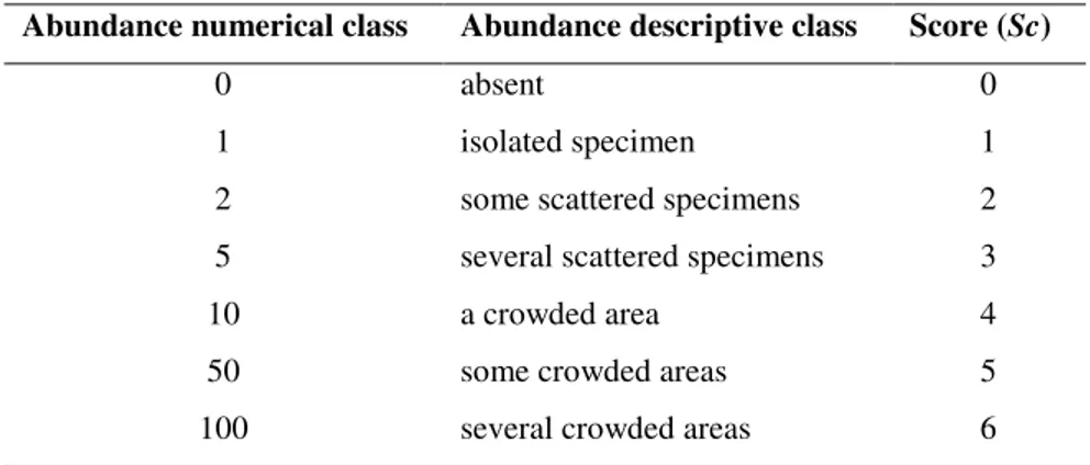
Table 2.2 Abundance class to score conversion.

Abundance numerical class Abundance descriptive class Score (Sc)

0 absent 0

1 isolated specimen 1

2 some scattered specimens 2

5 several scattered specimens 3

10 a crowded area 4

50 some crowded areas 5

100 several crowded areas 6

Mediterranean Reef Check Species richness ratio (MRC-Sratio) resembles the

species richness (S) and represents the proportion of taxa found compared to those searched (taxa searched). This index is based only on presence/absence species data.

MRC-Sratio = Taxa found / Taxa searched

The MRC-Sratio index ranges between 0 (no taxa found) and 1 (all searched taxa

were found). The maximum number of species that can be found is 43, according to the U-CEM protocol. However, the ratio between taxa searched and taxa found could be affected by the volunteer’s choices and by the amount of data available.

Mediterranean Reef Check Species diversity (MRC-D) resembles the

Simpson’s diversity index (1-D; Simpson 1949), which is considered one of the most meaningful and robust diversity measure available (Magurran 2004).

MRC-D = 1-∑pi2

where pi is the proportional abundance of the ith observation calculated on the

abundance class score (Sc).

Mediterranean Reef Check Species heterogeneity (MRC-H) resembles the

Shannon’s index (H’, Shannon & Weaver 1949) and mainly represents the overall heterogeneity of the searched taxa. Higher numbers indicate high species diversity and low numbers low species diversity.

MRC-H = ∑ (pi × log2pi)

where pi is the proportional abundance of the ith observation calculated on the

abundance class score (Sc).

The MRC-H index tends to vary from 0 to 5. The index allows to distinguish the differences between areas with the same number of species and with the same number of individuals, but in different proportion.

To meet the WFD and MSFD requirements, calculated indices should be classified in five ecological classes, corresponding to ecosystem health status. In the first instance, the index values obtained for each TUs were subjected to frequency distribution analysis (the Sturges’s algorithm was used to compute the numbers of classes to be used in the analysis, Sturges 1926) and tested for normality. If the data were normally distributed, the ecological class intervals were based on quintiles (i.e. five quantiles). This ensures that each class is equally represented (Evans 1977). When the distribution was bimodal or multimodal, natural breaks approach based on the Jenks optimization method (Jenks 1967) was used. This minimizes value differences among data within the same class and emphasizes the difference among the classes (Evans 1977). When the frequency distribution was homogeneous (rectangular), the class intervals were defined by dividing the range of values in equal intervals. A colour was assigned of each ecological class using red, orange, yellow, green and blue, in the order, to indicate increasing ecological status.

2.3.2 Non-indigenous species indices

Three easily recognisable NIS species are included in the RCI list of target taxa: two are green algae Caulerpa cylindracea Sonder, 1845 and Caulerpa taxifolia (M. Vahl) C. Agardh, 1817 and one is the gastropod mollusc Rapana venosa (Valenciennes, 1846). In order to assess the presence and abundance of these selected NIS, two simple indices were developed. To ensure the robustness of the indices, the following minimum requirements are imposed:

• minimum TU size: 0.25 km2

• minimum trained observers (i.e. diver volunteers): 3

• minimum number of observations (including absences): 10

For each observation, including absence, the abundance class were converted in abundance score class (Sc; Table 2.2).

Mediterranean Reef Check presence percentage (MRC- SPpresence %) represents

the percentage of sighting of the selected NIS compared to the number of times it was searched, including absences.

MRC-SPpresence % = (sightings / times searched)

The index is based only on presence/absence data.

Mediterranean Reef Check abundance percentage (MRC-SPabundance %)

represents the mean percentage abundance of the selected NIS. It is obtained through the sum of the abundance scores in case of sightings (Sc from 1 to 6; Table 2.2) divided by the sum of the abundance scores in case of sightings plus the count of absences recorded (i.e. Sc = 0).

in the U-CEM protocol, not only the NIS, therefore these indices could be also used for broad-scale species distribution analyses.

The index values, obtained for each TUs, were subjected to frequency distribution analysis and tested for normality. The indices values were classified in five classes, the first correspond to the absence (never sighted), the others values were divided in equal intervals ranging from 0 to 1. Considering the negative impact of the NIS, a colour was then assigned to each class using blue, green, orange, yellow and red, in the order, to indicate decreasing ecological status (i.e. increasing presence and abundance of NIS).

2.3.3 Species sensitive assessment

The present work mainly focus on subtidal rocky bottom and coralligenous habitats, therefore their most representative species included in the U-CEM taxa list were selected and further analysed. This selection resulted in a subset of 22 species and 3 genera (Table 2.3).

Following the approach of the Marine Life Information Network for Britain and Ireland (MarLIN, www.marlin.ac.uk; Hiscock 1997, Hiscock et al. 1999, Tyler-Walters & Jackson 1999, revised: January 2000, Hiscock et al. 2003), a sensitive assessment has been done for each of the sub selected taxon. MarLIN sensitive assessment approach is based on the review of available literature on the life history, distribution, environmental preference (Table 2.4) and any effects of disturbance agent on the chosen species (Hiscock & Tyler-Walters 2006).

Table 2.3 Taxa selected for the sensitive assessment and their typical habitats.

Taxon Typical habitats

Caulerpa cylindracea rocky bottom

Caulerpa taxifolia rocky bottom

Axinella spp. coralligenous

Aplysina spp. rocky bottom, cave

Geodia cydonium rocky bottom, detritic

Corallium rubrum coralligenous, cave

Paramuricea clavata coralligenous

Eunicella cavolinii coralligenous

Eunicella singularis coralligenous

Eunicella verrucosa soft bottom, coralligenous

Parazoanthus axinellae rocky bottom

Savalia savaglia coralligenous

Cladocora caespitosa coralligenous

Astroides calycularis rocky bottom

Balanophyllia europaea rocky bottom

Leptopsammia pruvoti coralligenous

Rapana venosa rocky bottom, artificial reef

Arca noae rocky bottom

Palinurus elephas coralligenous, cave

Homarus gammarus coralligenous, cave

Paracentrotus lividus rocky bottom

Hippocampus spp. seagrasses

Conger conger rocky bottom, wreck

Sciaena umbra rocky bottom

Chromis chromis rocky bottom

Table 2.4 General information need for assessment (MarLIN, www.marlin.ac.uk).

Taxonomy Phylum Class Order Family Genus Species Authority

Habitat information Physiographic preference Biological zone preferences Substratum/ habitat preferences Tidal strenght preferences Wave exposure preferences

General biology Typical abundance Male size range Male size at maturity Female size range Female size at maturity Growth form

Growth rate Body flexibility Mobility

Characteristic feeding methods Typically feeds on

Sociability

Environmental position Supports (Depend on/ support) Is the species toxic?

Reproduction and longevity Reproductive type Reproductive frequency Developmental mechanism Fecundity (number of eggs) Generation time

Age at maturity Dispersal potential Larval settling time Time of first gamete Time of last gamete Life span

Ecosystem importance Protection

Does the species create space in the assemblage? Does it occupy space and exclude?

Does the species provide habitat structure?

Does the species provide an important food source? For what? Medicinal use Aquaculture use Harvested (targered) Harvested (by-catch) Curio use Culinary use Threats

According to MarLIN (Hiscock et al. 2003, Hiscock & Tyler-Walters 2006), the sensitivity is the susceptibility of a species to be damaged, or die, from a disturb

revised: January 2000, Hiscock & Tyler-Walters 2006; Table 2.5). The recoverability is the ability of a species to redress damage sustained because of disturbance agents. On overall, the sensitivity is dependent on the intolerance of a species to be damaged from a disturbance agent and the time taken for its subsequent recovery (Tyler-Walters & Jackson 1999, revised: January 2000).

Table 2.5 Disturbance agents taking into consideration for evaluating the species sensitive (MarLIN, www.marlin.ac.uk).

Physical disturbs Substratum loss Smothering

Changes in suspended sediment Desiccation

Changes in emergence Changes in water flow rate Changes in temperature Changes in turbidity Changes in wave exposure Noise

Visual presence

Physical disturbance or abrasion Displacement

Chemical disturbs Changes in levels of synthetic chemicals Changes in levels of heavy metals Changes in levels of hydrocarbons Changes in levels of radionuclides Changes in levels of nutrients Changes in salinity

Changes in oxygenation

Biological disturbs Introduction of microbial pathogens and parasites Introduction of alien or non- native species Specific targeted extraction of this species Specific targeted extraction of other species

For each taxa and disturb agent, an intolerance and a recoverability value were attributed based on the MarLIN standard benchmarks (Tyler-Walters & Jackson 1999, revised: January 2000). The use of standard benchmarks allows sensitivity not only to be assessed relative to a specific change in an environmental factor but

a few days). Where the species is protected from the disturbance agent, the rating applies is “not relevant” both for the intolerance and for the recoverability (Hiscock et al. 1999). The species sensitivity toward each disturbance agent was established by combining the intolerance and recoverability ranks (Table 2.6).

Table 2.6 Combination between taxa intolerance and recoverability to obtain sensitivity (MarLIN, www.marlin.ac.uk).

Recoverability None Very low

(>25 yr) Low (>10/25 yrs) Moderate (>5/10 yrs) High (1/5 yrs) Very high (<1 yr) Immediate (<1 week) In to le ra n ce

High Very high Very high High Moderate Moderate Low Very Low Intermediate Very high High High Moderate Low Low Very Low Low High Moderate Moderate Low Low Very low NS

Tolerant NS NS NS NS NS NS NS

Tolerant* NS* NS* NS* NS* NS* NS* NS*

Not relevant NR NR NR NR NR NR NR

The sensitivity rank varies from “very high” to “not sensitive”. When the species is protected from the factor, the rank is “not relevant”. For detailed ranks definition see Hiscock et al. 1999, Tyler-Walters & Jackson 1999, revised: January 2000 and for further information about the MarLIN procedure applied see Hiscock 1997, Hiscock et al. 1999, Tyler-Walters & Jackson 1999, revised: January 2000, Hiscock et al. 2003, Hiscock & Tyler-Walters 2006 and the MarLIN website (www.marlin.ac.uk). Thus, the sensitive quality scores were converted in numerical scores (Table 2.7).

Table 2.7 Conversion between sensitive quality class and sensitive quantitative score (MarLIN, www.marlin.ac.uk).

Sensitive quality class Sensitive quantitative score

Very high 5 High 4 Moderate 3 Low 2 Very low 1 Not sensitive 0

sources on sensitivity and recoverability to a particular factor) to “very low” (i.e. informed judgment). “Not relevant” is used when no relevant information has been found or for insufficient information (Hiscock et al. 1999, Tyler-Walters & Jackson 1999, revised: January 2000).

The complete procedure used to assess taxa sensitivity includes the following steps (Fig. 2.1):

1. a review of relevant available information for the taxa in question;

2. collate key information;

3. the identification of the likely intolerance of the taxa to external factors;

4. the identification of the likely recoverability of the taxa to external factors;

5. the identification of the likely sensitivity of the taxa to external factors;

6. the conversion of the sensitivity judgment to a numeric value;

7. an assessment of the quality of the data used (confidence level);

8. the conversion of the confidence level to a numeric value;

9. peer review (referees comments and modification of conclusions if

2.3.4 Species sensitivity indices

In order to evaluate the ecological status of the Mediterranean rocky bottoms based on the sensitivity of species, the Mediterranean Reef Check Species sensitivity indices (MRC-Ss) suite was developed. According to the main group of disturbance agents listed in MarLIN, four indices were included in the suit. The

MRC-Species sensitive index toward physical disturbs (MRS-Ssphy), the

MRC-Species sensitive index toward chemical disturbs (MRS-Sschem) and the

MRC-Species sensitive index toward biological disturbs (MRS-Ssbio) were respectively

calculated on the mean sensitive value of each species toward physical (MSVphy),

chemical (MSVchem) and biological (MSVbio) disturbance factors. The overall

MRC-Species sensitivity index (MRC-Sstot) was calculated from the mean

sensitive value of each species toward each disturbance agent (MSVtot).

To ensure the robustness of the indices, the following minimum requirements are imposed:

• minimum TU size: 0.25 km2

• minimum trained observers (i.e. diver volunteers): 4

• minimum number of observations (including absences): 30

• minimum searched taxa: 15 (up to 25)

For each observation, including absence, the abundance class were converted in abundance score class (Sc; Table 2.2).

Mediterranean Reef Check Species sensitive index toward physical disturbs (MRC-Ssphy) mainly represents the mean sensitive value of the sighted taxa

toward physical disturbance factors (MSVphy), weighted by their observed

abundance class.

MRC-Ssphy= ∑ (Sci × MSV(phy)i ) / ∑ Sci

toward chemical disturbance factors (MSVchem), weighted by their observed

abundance class.

MRC-Sschem= ∑ (Sci × MSV(chem)i ) / ∑ Sci

where MSV(chem)irefers to the taxon in the ith observation.

Mediterranean Reef Check Species sensitive index toward biological disturbs (MRC-Ssbio) mainly represents the mean sensitive value of the sighted taxa toward

biological disturbance factors (MSVbio), weighted by their observed abundance

class.

MRC-Ssbio= ∑ (Sci × MSV(bio)i ) / ∑ Sci

where MSV(bio)irefers to the taxon in the ith observation.

Overall Mediterranean Reef Check Species sensitive index (MRC-Sstot) mainly

represents the mean sensitive value of the sighted taxa toward all possible

disturbance factors (MSVtot), weighted by their observed abundance class.

MRC-Sstot= ∑ (Sci × MSV(tot)i ) / ∑ Sci

where MSV(tot)irefers to the taxon in the ith observation.

All the indices theoretically range between 0 and 5, even if the extremes are impossible to achieve. They increase with increasing of the mean sensitivity of the species sighted and, in less extent, with their abundance.

The index values, obtained for each TUs, were subjected to frequency distribution analysis and tested for normality. The ecological class intervals were identified using quintiles among all the indices values obtained and a colour was then assigned to each class: blue, green, yellow, orange and red, in the order, to indicate increasing mean sensitivity of the assemblages.

intensities of human disturbances in the area. Greater the impacts, lower should be the sensitivity of the assemblages. Ideally, the indices should be tested in a wide range of condition, from highly impacted to pristine areas. Unfortunately, through the Mediterranean Sea is quite impossible to find pristine areas that can be used as reference conditions. Where undisturbed areas cannot be found historical data or experts’ judgment could represent theoretical reference condition (Andersen et al. 2004, Stoddard et al. 2006, Mangialajo et al. 2007). In the present study, the indices were compared with an assessment carried out with traditional methods within the Tavolara Capo Coda Cavallo MPA (Bianchi et al. 2012). In particular, the MPA Environmental quality map was used (www.amptavolara.com/en/home-page/). For the comparison, the area was divided in UTM grid cells, 500 m per side each. MRC-Ssi indices were calculated for each cell where enough data were available.

All the MRC indices, frequency distribution analyses and normality tests were calculated by routines write in R (R Core Team 2012). The Reshape (Wickham 2014), Vegan (Oksanen et al. 2015) and Normest R packages (Pearson chi-square

normality test, H0: the data are normally distributed, α = 0.05, Thode 2002, Gross

3

Results

3.1

Reliability of data collected by RCI volunteers

In order to assess the reliability of the RCI dataset, ability of divers with different training level were compared in a field test carried out at the Gallinara Island, which included 2 surveys and 10 independent observers. Patterns of similarities among observed assemblages are shown in the PCO ordination plot (Fig. 3.1). The first two axes of the PCO explained 34.8 and 28.9% of the total variation. The scatter plot shows some degrees of separation between the two sites, but not among the observer training levels.

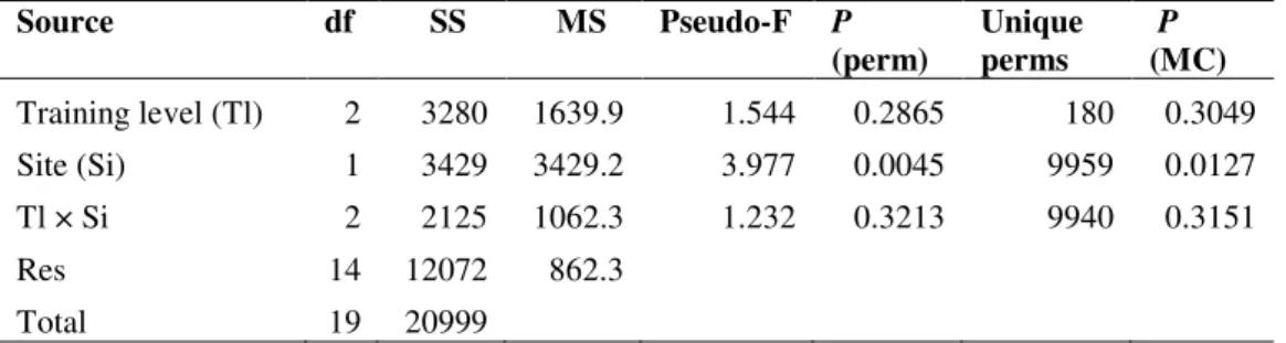
The pattern was confirmed by the PERMANOVA test, showing significant difference only between sites not among training levels (Table 3.1). Even if some minor differences among operators were obtained (points in the PCO are not exactly coincident), these represent a random effect related to the accuracy of the method, as occurs in any visual census. Therefore, the method appeared quite robust, able to distinguish assemblages between sites, and not affected by the training levels of the operators. In other words, the minimum training provided by RCI appears adequate.

Table 3.1 Results from PERMANOVA on Bray-Curtis similarities abundance data

Source df SS MS Pseudo-F P (perm) Unique perms P (MC) Training level (Tl) 2 3280 1639.9 1.544 0.2865 180 0.3049 Site (Si) 1 3429 3429.2 3.977 0.0045 9959 0.0127 Tl × Si 2 2125 1062.3 1.232 0.3213 9940 0.3151 Res 14 12072 862.3 Total 19 20999

3.2

RCI database contents

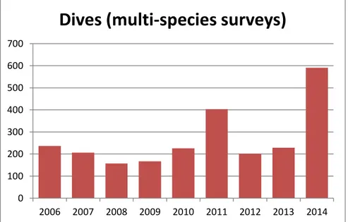
At the last data mining (22/05/2015), the whole RCI database includes 31’190 observations, including absences, carried out in 3’585 surveys (i.e. individual dives). That includes several data collected before the establishment of the current U-CEM protocol and/or without fulfilling the U-CEM standard. Limiting the dataset to the interval 2006-2014 and excluding data with not satisfy the U-CEM standard, 24’966 observation in 2’434 survey were retained for further analyses. In the 2014, the number of surveys (Fig. 3.2) and observations (Fig. 3.3) were largely increased compared to the previous years, which could be related to a relevant increase of EcoDiver volunteers in the last year (Fig. 3.4). On average, each EcoDiver investigate 10.23 ± 0.19 s.e. taxa and spend 35.2 ± 0.4 s.e. minutes per dive.

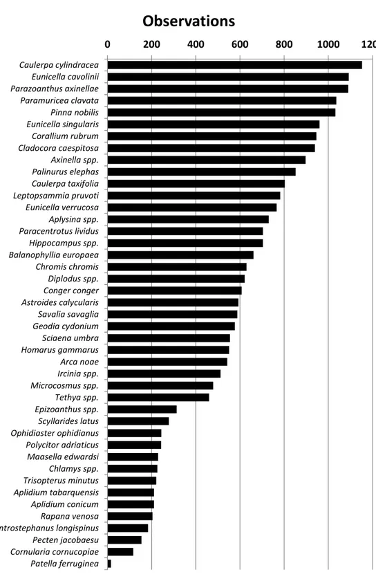
put more efforts in searching the most attractive species, including those to which there is greater awareness, like NIS (Fig. 3.7).

Fig. 3.2 Surveys annually carried out between 2006 and 2014.

Fig. 3.3 Observations annually recorded between 2006 and 2014. 0 100 200 300 400 500 600 700 2006 2007 2008 2009 2010 2011 2012 2013 2014

Dives (multi-species surveys)

0 1000 2000 3000 4000 5000 6000 7000 8000 2006 2007 2008 2009 2010 2011 2012 2013 2014

Observations

Fig. 3.4 Participating EcoDivers between 2006 and 2014.

Fig. 3.5 Surveys distribution per habitats. 0 50 100 150 200 250 300 350 400 2006 2007 2008 2009 2010 2011 2012 2013 2014 Tot

Contributing Divers

Fig. 3.7 Observation effort distribution among taxa. 0 200 400 600 800 1000 1200 Patella ferruginea Cornularia cornucopiae Pecten jacobaesu Centrostephanus longispinus Rapana venosa Aplidium conicum Aplidium tabarquensis Trisopterus minutus Chlamys spp. Maasella edwardsi Polycitor adriaticus Ophidiaster ophidianus Scyllarides latus Epizoanthus spp. Tethya spp. Microcosmus spp. Ircinia spp. Arca noae Homarus gammarus Sciaena umbra Geodia cydonium Savalia savaglia Astroides calycularis Conger conger Diplodus spp. Chromis chromis Balanophyllia europaea Hippocampus spp. Paracentrotus lividus Aplysina spp. Eunicella verrucosa Leptopsammia pruvoti Caulerpa taxifolia Palinurus elephas Axinella spp. Cladocora caespitosa Corallium rubrum Eunicella singularis Pinna nobilis Paramuricea clavata Parazoanthus axinellae Eunicella cavolinii Caulerpa cylindracea

Observations

3.3

Mediterranean Reef Check Diversity indices

The MRC-Sratio index values calculated for provincial coastal areas ranged from

0.17 to 0.96 (Annex 1) and were normally distributed (Pearson chi-square normality test, p = 0.74) (Fig. 3.8).

Fig. 3.8 Frequency distribution of MRC-Sratioindex values in the coastal provinces.

Five classes of equal intervals were chosen and a possible interpretation scale for species richness ratio and ecological status was proposed (Table 3.2). The highest obtained values were in the province of Genoa, Grosseto, Reggio Calabria, Savona and Trapani as it shows in blue colour in the map (Fig. 3.9). The lowest value was in Messina where only 4 out of the 24 searched species were found.

Table 3.2 Proposed classification scheme for the MRC-Sratio index.

MRC-Sratio Species richness ratio Ecological status

0.00 – 0.20 Very low Bad

0.20 – 0.40 Low Poor

0.40 – 0.60 Mean Moderate

0.60– 0.80 High Good

0.80 – 1.00 Very high High

Fig. 3.9 MRC-Sratio index values in the coastal provinces (Mercator projection,

WGS84).

There is no linear correlation between obtained index values and taxa searched (p

= 0.06, r = 0.36 R2 = 0.08) therefore it could be excluded that volunteers choices

normality test, p = 4.69e-06) (Fig. 3.10). The natural breaks were used to define five classes and a possible interpretation scale for species diversity and ecological status is proposed in Table 3.3.

Fig. 3.10 Frequency distribution of MRC-D index values in the coastal provinces.

Table 3.3 Proposed classification scheme for the MRC-D index. MRC-D Species diversity Ecological status 0.00 – 0.69 Very low Bad

0.69 – 0.72 Low Poor

0.72 – 0.89 Mean Moderate

0.89 – 0.94 High Good

0.94 – 1.00 Very high High

Fig. 3.11 MRC-D index values in the coastal provinces (Mercator projection, WGS84).

3.3.3 Mediterranean Reef Check Species heterogeneity index

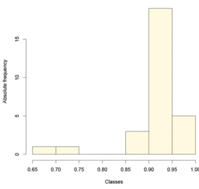
The MRC-H index values calculated for provincial coastal areas ranged from 1.86 (Messina province) to 4.70 (Savona province) (Annex 1) and were normally distributed (Pearson chi-square normality test, p = 0.05) (Fig. 3.12).

Fig. 3.12 Frequency distribution of MRC-H index values in the coastal provinces.

Five classes using quintiles were chosen and a possible interpretation scale for species heterogeneity and ecological status was proposed in Table 3.4.

Table 3.4 Proposed classification scheme for the MRC-H index. MRC-H Species heterogeneity Ecological status

0.00 – 3.32 Very low Bad

3.32 – 4.00 Low Poor

4.00 – 4.30 Mean Moderate

4.30 – 4.54 High Good

4.54 – 5.00 Very high High

Provinces with the highest values were Grosseto, Livorno, Naples and Savona. However, most provinces fall in the mean range with moderate ecological status

Fig. 3.13 MRC-H index values in the coastal provinces (Mercator projection, WGS84).

3.4

Mediterranean Reef Check NIS indices

A possible interpretation scale for species presence (sighting frequency) and mean abundance, which can be applied for any species, and a corresponding ecological status in case of NIS was proposed (Table 3.5). It was based on the confirmed absence and 4 equal intervals of percentage.

Table 3.5 Proposed classification scheme for the MRC-SP indices. MRC-SPpresence %

MRC-SPabundance %

sighting frequency mean abundance Ecological status (NIS)

0 – 0 Absent Absent High

0 – 25 Rare Rare Good

3.4.1 Caulerpa cylindracea

The MRC-C.cylindraceapresence % index values calculated for provincial coastal

areas ranged from 0 to 0.94, while the MRC-C.cylindraceaabundance % index values

from 0 to 0.98 (Annex 2). The MRC-C.cylindraceapresence % index values were

normally distributed (Pearson chi-square normality test, p = 0.86), while

MRC-C.cylindraceaabundance % index values were not normally distributed (Pearson

Fig. 3.14 Frequency distribution of MRC-SP indices values obtained for C. cylindracea.

C. cylindracea was introduced in the Mediterranean Sea from south-western

Australia in the early ‘90s (Klein & Verlaque 2008). Its first record in the Mediterranean Sea comes from Libya in 1990 and the primary vehicle of introduction could be attributed to maritime traffic or aquaria trade (Klein & Verlaque 2008). The species is rapidly spreading across the Mediterranean via both sexual and vegetative reproduction and thanks to shipping, fishing and currents, dramatically altering the local benthic communities (Klein & Verlaque 2008). Nowadays, this species are present in many Italian coastal zones as confirmed by the map (Fig. 3.15). The most affected provinces are in Liguria, Tuscany, Sicily, and Apulia Regions. In particular, along the coast of the Liguria Region first records of C. cylindracea come from the province of Genoa from Quinto and date back to 1995 (Bussotti et al. 1996). Thereafter, some records have been reported the spread of C. cylindracea from east to west Ligurian coast (Montefalcone et al. 2007a, Montefalcone et al. 2007b, Piazzi et al. 2005, Tunesi et al. 2007).

Fig. 3.15 MRC-SP indices values in the coastal provinces (Mercator projection, WGS84).

index values were not normally distributed (Pearson chi-square normality test,

ppresence % = 3.16e-05 and pabundance % = 4.75e-05) (Fig. 3.16).

Fig. 3.16 Frequency distribution of MRC-SP indices values obtained for C. taxifolia.

The green algae C. taxifolia in the Mediterranean Sea has spread steadily since its introduction in 1984 from the aquarium in Monaco (Meinesz & Hesse 1991, Boudouresque et al. 1995). At the end of 2000, it has colonized thousands of hectares mainly in six Mediterranean countries: Spain, France, Monaco, Italy, Croatia and Tunisia (Relini et al. 2000). In Italy the first discovery of C. taxifolia was made in 1992 in Imperia (GE) harbour (Relini & Torchia 1992). Nowadays it is recorded in Liguria, Tuscany, Sicily and Calabria (Meinesz et al. 2001).

The indices show the absence of C. taxifolia along some Adriatic and southern Italian coasts, where enough data were collected. Although C. taxifolia issue has been extensively reported in magazine and scientific journals (Klein & Verlaque 2008), its distributional pattern appeared less concerned than C. cylindracea ones along the Italian coasts (Fig. 3.17).

Fig. 3.17 MRC-SP indices values in the coastal provinces (Mercator projection, WGS84).