Corso di Laurea Magistrale in
Ingegneria Energetica
AN INTEGRATED THERMODYNAMIC/CFD APPROACH
TO EJECTOR MODELING
Relatore:
Prof. Paolo Chiesa
Co-relatore: Ing. Riccardo Mereu
Tesi di Laurea di:
Giorgio Besagni
Matricola 759956
This work is dedicated to my father my mother my sister in memory of my grandfather Ennio my grandmother Maria “Voici mon secret. Il est très simple: on ne voit bien qu'avec le cœur. L'essentiel est invisible pour les yeux.”
i
Acknowledgments
Il ringraziamento più grande lo devo alla mia famiglia, perché se sono arrivato fino a questo giorno lo devo a loro, ai loro sorrisi, al loro sostegno e affetto.
Ringrazio il mio relatore, il Professor Paolo Chiesa, per il tempo che mi ha dedicato, per la pazienza e l’umanità. Ringrazio molto anche la Professoressa Emanuela Colombo per i consigli e la gentilezza. A loro va il merito del dottorato che inizierò.
Doveroso il ringraziamento a Riccardo, per come mi ha seguito in questi mesi, per i consigli, le osservazioni, la pazienza e l’immancabile buon umore.
Ringrazio il Professor Fabio Inzoli e tutti i miei futuri colleghi di dottorato, per come mi hanno accolto nell’ambiente del gruppo di ricerca.
Grazie a Marco, per l’amicizia di questi anni, per essermi sempre stato a ascoltare, per le camminate e i consigli.
Grazie a Matteo, compagno di corso e amico in questi anni di università, lo ringrazio per l’immensa pazienza, i consigli, i discorsi. Cinque anni di corsi, con un amico così, sono pesati meno.
Grazie alla mia squadra di Croce Rossa, il Mercoledì notte, perché se ogni volta che mi metto la divisa sono sempre di buon umore, lo devo in buona parte a voi. Grazie Adriano, Daniele, Laura, Rosy, Paola, Claudia Z. e Claudia L.L. Siete grandi.
Grazie a Enzo, per il continuo sostegno e perché molto di quello che ho imparato come volontario, soccorritore e persona lo devo in buona parte a te.
Grazie a Piero perché mi ha insegnato che il vero cammino comincia quando finisce la strada.
Grazie ai compagni di viaggio, per i chilometri percorsi insieme. In particolare a Giorgio, Riccardo, Roberto, Sergio ed Elisa.
Grazie agli amici di lunga data Lorenzo, Riccardo e Giulia, perché non mi serve vedervi spesso per sapere che posso contare su di voi.
Grazie a tutte le persone che in questi anni mi hanno accompagnato e che ora hanno presto strade diverse. Molto devo anche a loro.
iii
Abstract
Ejectors are widely used in energy engineering and, from the first half of the twentieth century, a large amount of studies have been conducted on modeling and analyzing ejectors by using thermodynamic and Computational Fluid-Dynamics(CFD) approaches. Both modeling techniques have advantages and limits: the former ensures limited computational time and less cost than experimental method for predicting ejector performance, but it is unable to describe internal flow behavior; the latter is able to provide deep understanding of local phenomena, but it requires a higher computational cost and specific competencies in numerical methods. The integrated thermodynamic/CFD approach, proposed in this thesis, defines guidelines and proposes a novel ejectors model that, combining advantages of both described techniques, has potentiality of predicting ejectors performance, accounting local flow behavior. This approach will be applied to the case of a single phase subsonic ejector, providing a model with a structure ready to be implemented in energy power plant simulation codes. In order to achieve this result the thesis is structured as follow: in the first chapters, a description of ejector technology and a review of its modeling state-of-the-art will be provided. In the second pstate-of-the-art the structure of the novel thermodynamic model and the CFD approach will be outlined. The section related with the computational model validation is composed by a comparison of different turbulence models for subsonic ejector and by the description of a qualified approach for numerical investigation requiring application of best practices and software recommendations (the Q3 approach is used, which include the three interdependent, but related, dimensions: software reliability, user knowledge and process control). At the end, the integration of these two modeling approaches will be described and commented.
Keywords: ejector technology; ejector modeling; convergent nozzle; under-expanded jets; CFD; RANS turbulence models;
v
Italian abstract
Gli eiettori trovano largo impiego nell’ingegneria energetica e, dalla prima metà del ventesimo secolo, sono stati presentati molti lavori sulla loro modellazione e analisi, usando sia un approccio termodinamico che uno basato sulla termo fluidodinamica computazionale (CFD). Entrambe queste tecniche hanno vantaggi e limiti: la prima assicura tempi di calcolo e costi minori rispetto a analisi sperimentali, a fronte di un’incapacità nel descrivere il campo di moto interno; la seconda è idonea alla descrizione di fenomeni locali, ma richiede maggiori oneri computazionali e specifiche competenze nell’ambito dei metodi numerici. L’approccio integrato termodinamico/CFD, proposto in questa tesi, definisce linee guida e propone un nuovo modello per eiettori che, riunendo i vantaggi di entrambe queste tecniche, ha la potenzialità di predire le prestazioni di eiettori tenendo in considerazione i fenomeni fluidodinamici locali. Questo approccio sarà applicato a un eiettore subsonico con flusso monofase, presentando un modello con una struttura facilmente implementabile in codici per la simulazione di impianti di potenza. Per arrivare a questo risultato la tesi è strutturata come segue: nei primi capitoli è presentata una descrizione della tecnologia degli eiettori e una presentazione sullo stato dell’arte della loro modellazione. Nella seconda parte è presentata la struttura del nuovo modello termodinamico e dell’approccio CFD. La sezione relativa alla validazione del modello numerico è costituita dal confronto delle prestazioni di modelli di turbolenza RANS per eiettori subsonici e dalla descrizione di un approccio qualificato che richiede l’applicazione delle migliori pratiche e competenze sull’utilizzo del software (è utilizzato l’approccio Q3, che include tre dimensioni indipendenti ma collegate: l’affidabilità del software, la competenza dell’utente e il controllo del processo). In conclusione sarà descritta e commentata l’integrazione di questo due approcci modellistici.
Italian keywords: tecnologia degli eiettori; modellazione degli eiettori; ugello convergente; getti sotto-espansi; CFD; modelli di turbolenza RANS.
vii
Contents
ACKNOWLEDGMENTS ... I ABSTRACT ... III ITALIAN ABSTRACT ... V CONTENTS ... VII LIST OF FIGURES ... X LIST OF TABLES ... XIIIINTRODUCTION ... 1 EJECTOR TECHNOLOGY ... 3 CHAPTER 1 1.1CLASSIFICATION ... 3 1.2OPERATING CONDITIONS... 4 1.2.1 Supersonic ejectors ... 4 1.2.2 Subsonic ejectors ... 4
1.3APPLICATIONS IN ENERGY FIELD... 5
1.3.1 Supersonic ejector applications in energy field ... 5
1.3.1.1 Refrigeration ... 6
1.3.1.2 SOFC and MCFC power plants ... 7
1.3.2 Subsonic ejector applications in energy field ... 8
1.3.2.1 PEMFC ... 8
1.3.2.2 CLC ... 10
EJECTOR MODELING ... 11
CHAPTER 2 2.1INTRODUCTION TO EJECTOR MODELING: MODELS STRUCTURE ... 11
2.1.1 Approach ... 11
2.1.2 Fundamental hypothesis of thermodynamic models ... 11
2.1.3 Equations to be solved ... 12
2.1.4 Boundary conditions ... 13
2.1.5 Initial conditions ... 13
2.1.6 Turbulence modeling ... 13
2.1.7 Auxiliary relations ... 14
2.2THERMODYNAMIC EJECTOR MODELING: STORY AND CURRENT STATE-OF-THE-ART ... 15
2.2.1 A brief story on thermodynamic ejector modeling... 15
2.2.2 Subsonic ejector modeling: a recent theme of research ... 22
2.2.3 Limitations of thermodynamic models ... 30
2.3EJECTOR EFFICIENCIES AND THEIR ROLE IN THERMODYNAMIC MODELING... 31
2.3.1 Ejector global efficiency. ... 31
2.3.2 Ejector efficiencies ... 32
2.3.2.1 Primary Nozzle ... 33
2.3.2.2 Suction nozzle ... 33
2.3.2.3 Aerodynamic throat ... 34
viii
2.3.2.5 Diffuser ...37
2.3.2.6 Ejector efficiencies used in literature ...37
2.3.3 Role of the integrated thermodynamic/CFD model ...39
2.4CFD EJECTOR MODELING: STORY AND CURRENT STATE-OF-THE-ART ...39
2.4.1 A brief story on CFD ejector modeling ...39
2.4.2 Guidelines in CFD ejector modeling ...41
THERMODYNAMIC MODEL ...47
CHAPTER 3 3.1BASIS OF THE NOVEL THERMODYNAMIC MODEL ...47
3.1.1 Power plant simulation codes constrains and modification over the typical 1D approach ...47
3.1.2 CFD contributions ...48
3.2DESCRIPTION OF THE NOVEL THERMODYNAMIC MODEL ...49
3.2.1 Hypothesis ...49
3.2.2 Input...49
3.2.3 Preliminary calculations: flow compositions ...50
3.2.4 Primary nozzle ...51
3.2.5 Exit suction zone ...53
3.2.6 Mixing ...54 3.2.7 Diffuser ...56 3.3BASIS OF INTEGRATION ...56 CFD MODEL ...57 CHAPTER 4 4.1Q3APPROACH ...57 4.1.1 Introduction ...57 4.2.2 Protocol structure ...57
4.2CFD CYCLE PHASE 1-PROBLEM ANALYSIS ...58
4.2.1 Frame of action and general purposes ...58
4.2.2 Problem identification ...58
4.3CFD CYCLE PHASE 2- CONCEPTUAL MODEL SETTING: RESULTS AND APPROACH ...59
4.3.1 Specific goals of the CFD analysis ...59
4.3.2 State-of-the-art of CFD in the field ...59
4.3.3 Expected results and benchmark used ...59
4.3.4 General approach: main assumption and working hypothesis ...60
4.3.5 Activities and plan ...60
4.4CFD CYCLE PHASE 3– MODEL BUILDING AND SOLVING: DEPLOYMENT ...61
4.4.1 Pre-processing ...61
4.4.1.1 Domain identification and Geometry setting ...61
4.4.1.2 Mesh strategy and generation ...62
4.4.2 Model setting ...66 4.4.2.1 Solver ...66 4.4.2.2 Turbulence approach ...66 4.4.2.3 Physical properties ...67 4.4.2.4 Operating conditions ...67 4.4.2.5 Boundary conditions ...67 4.4.3 Numerical setting ...69 4.4.3.1 Numerical strategy ...69 4.4.3.2 Convergence control ...70
ix
4.5.1 Calculation verification ... 71
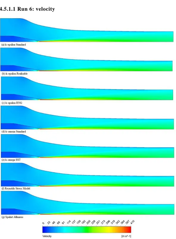
4.5.1.1 Run 6: velocity ... 73
4.5.1.2 Run 7: velocity ... 78
4.5.1.3 Run 9: Velocity ... 83
4.5.1.4 Run 9: Total Temperature ... 89
4.5.1.5 Run 10: velocity ... 92
4.5.2 Calculation validation and critical review of the model ... 96
4.5.3 Strategy improvement ... 96
4.6IMPORTANT REMARKS ... 96
4.6.1 Turbulence models performance comparison ... 96
4.6.1.1 Convergence behavior ... 97
4.6.1.3 Flow field (comparison with velocity data) ... 97
4.6.1.2 Thermal field (comparison with temperature data) ... 98
4.6.1.4 Results ... 99
4.6.2 Approach and guidelines for CFD ejector modeling. ... 99
4.6.3 Applications ... 100
INTEGRATION ... 101
CHAPTER 5 5.1PART 1: APPLICATION OF THE CFD APPROACH ... 101
5.1.1 Range of analysis ... 101
5.1.1.1 Primary range of analysis: primary mass flow rate variation ... 101
5.1.1.2 Secondary range of analysis: secondary mass flow rate variation. ... 102
5.2.2 Results ... 104
5.2.2.1 Efficiencies ... 104
5.2.2.2 Flow behavior ... 106
5.2PART 2: THE RELATIONSHIP BETWEEN INTERNAL FLOW AND EFFICIENCIES. ... 116
5.2.1 Nozzle ... 116
5.2.2 Suction ... 121
5.2.3 Mixing... 125
5.3PART 3: THE INTEGRATED THERMODYNAMIC/CFD MODEL FOR SINGLE PHASE SUBSONIC EJECTOR ... 135
5.3.1 Initialization ... 135
5.3.2 Thermodynamic model code ... 135
5.3.3 CFD efficiency LOOPs ... 135
5.3.4 Model structure ... 135
CONCLUSIONS ... 137
x
List of figures
Figure 1-1 Ejector layout; taken from [27] ... 3
Figure 1-2 Operation modes of supersonic ejector; taken from [30] ... 4
Figure 1-3 Operation modes of subsonic ejector; modified from [25] ... 5
Figure 1-4 JRC layout; taken from [41] ... 6
Figure 1-5 Rolls-Royce fuel cell system ... 7
Figure 1-6 PEM based system studied by [25] ... 9
Figure 1-7 PEM based system studied by [54] ... 9
Figure 1-8 (a) ejectors used on both Air Reactor and Fuel Reactor lines [56] and (b) ejector used on Fuel Reactor line only. ...10
Figure 2-1 Density contour on nozzle outlet (Simulation run 9, section 4.5.1.3) ...12
Figure 2-2 (a) Velocity distribution and (b) mixing section; taken from [75] ...17
Figure 2-3 Ejector studied by Zhu et al. [25] ...25
Figure 2-4 Radial velocity distribution in zone 2; taken from [25] ...27
Figure 2-5 Subsonic ejector operating condition; taken from [55] ...29
Figure 2-6 Ejector flow field; taken from [130] ...43
Figure 2-7 Effects of a mesh improvement; modified from [24] ...44
Figure 2-8 Turbulence modeling results comparison: (a) and (b) model ...44
Figure 3-1 Ejector studied ...47
Figure 4-1 Protocol structure; modified from [118]...58
Figure 4-2 Activities and plan ...61
Figure 4-3 Ejector geometry; taken from [137] ...62
Figure 4-4 Benchmark ejector; taken from [119]. ...62
Figure 4-5 2D Mesh used in previous work; taken from [119] ...63
Figure 4-6 Comparison between mesh (Figure 4-5) used and geometry in [137] ...63
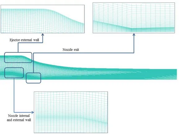
Figure 4-7 Mesh developed with GAMBIT ...64
Figure 4-8 Mesh developed with GAMBIT with details ...64
Figure 4-9 Aspect ratio comparison ...65
Figure 4-10 Cell surface comparison ...65
Figure 4-11 Element skewness comparison ...66
Figure 4-12 Boundary conditions used ...68
Figure 4-13 Mixing sections traverse locations; taken from [137] ...72
Figure 4-14 Velocity contours (run 6) ...73
Figure 4-15 Velocity profiles at (run 6) ...74
Figure 4-16 Velocity profiles at (run 6) ...74
Figure 4-17 Velocity profiles at (run 6) ...75
Figure 4-18 Velocity profiles at (run 6) ...75
Figure 4-19 Considerations about velocity profiles at (run 6)...76
Figure 4-20 Considerations about velocity profiles at (run 6)...77
Figure 4-21 Velocity contours (run 7) ...78
Figure 4-22 Velocity profiles at (run 7) ...79
Figure 4-23 Velocity profiles at (run 7) ...79
Figure 4-24 Velocity profiles at (run 7) ...80
Figure 4-25 Velocity profiles at (run 7) ...80
xi Figure 4-27 Run 7 nozzle exit velocity contours for (a) and (b)
... 82
Figure 4-28 Velocity contours (run 9) ... 83
Figure 4-29 Velocity profiles at (run 9) ... 84
Figure 4-30 Velocity profiles at (run 9) ... 84
Figure 4-31 Velocity profiles at (run 9) ... 85
Figure 4-32 Velocity profiles at (run 9) ... 85
Figure 4-33 Velocity profiles at (run 9) ... 86
Figure 4-34 Velocity profiles at (run 9) ... 86
Figure 4-35 Considerations about velocity profiles at (run 9) ... 87
Figure 4-36 Total temperature contours (run 9) ... 89
Figure 4-37 Total temperature profiles at (run 9) ... 90
Figure 4-38 Total temperature profiles at (run 9) ... 90
Figure 4-39 Run 9 nozzle exit total temperature contours for (a) and (b) ... 91
Figure 4-40 Velocity contours (run 10) ... 92
Figure 4-41 Velocity profiles at (run 10) ... 93
Figure 4-42 Velocity profiles at (run 10) ... 93
Figure 4-43 Velocity profiles at (run 10) ... 94
Figure 4-44 Velocity profiles at (run 10) ... 94
Figure 4-45 CFD cyclic process ... 96
Figure 4-46 Total temperature profiles at (run 9) ... 98
Figure 4-47 Total temperature profiles at (run 9) ... 99
Figure 5-1 Relations between primary mass flow rate variations, primary inlet pressure and primary inlet velocity ... 107
Figure 5-2 Simulation results: Mach contours. ... 108
Figure 5-3 Subsonic jet flow from a sonic nozzle; taken from [143] ... 109
Figure 5-4 Moderately under-expanded jet flow from a sonic nozzle; taken from [143] ... 110
Figure 5-5 Highly under-expanded jet flow from a sonic nozzle; taken from [143] ... 110
Figure 5-6 NPR=1.893; taken from [136] ... 111
Figure 5-7 NPR=2.50; taken from [136] ... 111
Figure 5-8 NPR=2.75; taken from [136] ... 111
Figure 5-9 NPR=3.00; taken from [136] ... 111
Figure 5-10 NPR=3.10; taken from [136] ... 112
Figure 5-11 NPR=4.00; taken from [136] ... 112
Figure 5-12 Relations between primary mass flow rate variations, secondary inlet pressure, secondary inlet velocity ... 113
Figure 5-13 Simulation results: Effects of improving (CASE11) - Mach contours ... 114
Figure 5-14 Simulation results: Effects of improving (run9) - Mach contours ... 115
Figure 5-15 Simulation results: Effects of improving (CASE2) - Mach contours ... 115
Figure 5-16 Nozzle efficiencies 3D plot ... 116
Figure 5-17 Nozzle efficiencies 2D plot ... 117
Figure 5-18 Nozzle efficiencies relationship with flow fields (part a) ... 118
Figure 5-19 Nozzle efficiencies relationship with flow fields (part b) ... 119
Figure 5-20 Error between CFD nozzle efficiencies and interpolating function proposed ... 120
Figure 5-21 Suction efficiencies 3D plot ... 121
Figure 5-22 Suction efficiencies 2D plot with considerations ... 122
xii
Figure 5-24 Error between CFD suction efficiencies and interpolating function proposed ...124
Figure 5-25 Mixing efficiencies ...125
Figure 5-26 Mixing efficiencies 2D plot with considerations ...126
Figure 5-27 Mixing efficiencies relationship with flow fields (part a) ...127
Figure 5-28 Mixing efficiencies relationship with flow fields (part b) ...128
Figure 5-29 Mixing efficiencies relationship with flow fields (part c) ...129
Figure 5-30 Mixing efficiencies relationship with flow fields (part d) ...130
Figure 5-31 Mixing efficiencies relationship with flow fields (part e) ...131
Figure 5-32 Interpolating surface ...132
Figure 5-33 Mixing efficiencies relationship with flow fields (with interpolating surface) ...133
Figure 5-34 Error between CFD mixing efficiencies and interpolating function proposed ...134
xiii
List of tables
Table 2-1 Relevant studies about thermodynamic model for supersonic single phase ejectors ... 22
Table 2-2 Relevant studies about thermodynamic model for subsonic single phase ejectors ... 30
Table 2-3 Value of parameters for [77] ... 34
Table 2-4 Value of parameters for [71] ... 35
Table 2-5 Mixing efficiencies; taken from [63] ... 36
Table 2-6 Ejector efficiencies: a brief overview... 38
Table 2-7 Experimental flow visualization studies ... 43
Table 4-1 Operating conditions of tests performed by Gilbert and Hill [137] ... 60
Table 4-2 Solver settings ... 66
Table 4-3 Working fluid properties ... 67
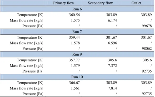
Table 4-4 Operating conditions taken from [137] ... 67
Table 4-5 Boundary condition for temperature, mass flow rate and pressure ... 68
Table 4-6 Boundary conditions for turbulence ... 69
Table 4-7 Numerical setting used... 70
Table 4-8 Control parameter used ... 70
Table 4-9 Comparison between experimental data and simulation results for data point , and ... 76
Table 4-10 Comparison between experimental data and simulation results for data point, , and ... 77
Table 4-11 Comparison between experimental data and simulation results ... 77
Table 4-12 Comparison between experimental data and simulation results for data point , and ... 82
Table 4-13 Comparison between experimental data and simulation results for data point , and ... 82
Table 4-14 Comparison between experimental data and simulation results ... 82
Table 4-15 Comparison between experimental data and simulation results for data point , and ... 87
Table 4-16 Comparison between experimental data and simulation results ... 88
Table 4-17 Comparison between experimental data and simulation results ... 88
Table 4-18 Comparison between experimental data and simulation results for data point , and ... 91
Table 4-19 Comparison between experimental data and simulation results for data point , and ... 91
Table 4-20 Comparison between experimental data and simulation results ... 95
Table 5-1 Primary range of analysis... 102
Table 5-2 Secondary range of analysis ... 103
Table 5-3 Efficiency results ... 106
Table 5-4 Coefficients of nozzle efficiency interpolating function ... 120
Table 5-5 Coefficients of suction efficiency interpolating function ... 124
1
Introduction
Ejectors are widely used in energy engineering for: (i) refrigeration applications [1], [2], (ii) fuel cells based systems [3], and (iii) advanced energy conversion power plants [4], [5], [6]. So, from the first half of the 20th century, beside experimental investigations [7], [8], [9], [10], [11], [12], [13], [14], [15], [16], [17], [18], [19], [20], [21] a large amount of works has been conducted on modeling and analyzing ejectors by using thermodynamic and Computational Fluid-Dynamics (CFD) approaches [22]. Both modeling techniques have advantages and limits: the former ensures limited computational time and less cost than experimental method for predicting ejector performance, but it is unable to describe internal flow behavior; the latter is able to provide deep understanding of local phenomena, but it requires a higher computational cost and specific competencies in numerical methods [23].
However, He et al. [23], after studying progress of mathematical modeling on ejectors, concluded that, though a large amount of studies have been presented on ejector modeling, further efforts are still needed:
1. to study the influence of variable isentropic coefficients, which are taken as constant in almost all existing thermodynamic models;
2. to improve the accuracy of the models based on turbulence modeling;
3. to build a simulation package of the whole ejector-based system by combining the model of the ejector and other components in the system.
This thesis starts from above remarks and proposes an ejector integrated thermodynamic/CFD modeling approach which will be applied to a single phase subsonic ejector.
The goals of this integrated approach are:
1. giving guidelines on CFD ejectors modeling;
2. providing efficiencies maps using a validated CFD approach;
3. proposing a novel thermodynamic model that uses efficiencies maps given by CFD simulations: this model will provide global parameters by considering local flow behavior;
4. developing a thermodynamic model ready to be integrated in energy power plant simulation codes;
Moreover, the application of the integrated approach to a single phase subsonic ejector will provide:
2
1. the first study focused on comparison of different turbulence models for the case of a convergent nozzle-ejector (in literature there are only studies about comparison of turbulence models for supersonic ejectors [24]);
2. further development for subsonic ejector modeling, which is an uncharted field of study [25].
In the next chapters a description of ejector technology (Chapter 1) and a review of ejector modeling state-of-the-art (Chapter 2) will be provided. In the second part the structure of the novel thermodynamic model (Chapter 3) and the CFD model (Chapter 4) will be discussed. In the third part of the thesis the integration of these two modeling approaches will be described and commented (Chapter 5). At the end, conclusions and future developments will be outlined.
3
Ejector technology
Chapter 1
Ejector, also known as injector or jet pump is a device constituted by a primary nozzle, a suction chamber, a mixing chamber and a diffuser (Figure 1-1) [26].
Figure 1-1 Ejector layout; taken from [27]
A high total energy “primary fluid” or “motive fluid”, expands and accelerates through the primary nozzle, flows out and creates a low pressure region at the nozzle exit plane and, subsequently, in the suction/mixing chamber. Hence, a “secondary fluid” or “entrained fluid” is drawn by both the entrainment effect (due to pressure reduction around nozzle exit) and the shear action between the primary and secondary fluids. By the end of the mixing chamber the two streams are completely mixed and a compression of the flow is achieved through a subsonic diffuser.
1.1 Classification
There are three ways of classifying ejectors:
1. supersonic and subsonic ejectors, according to the design of the nozzle:
subsonic ejectors: if nozzle is a converged;
supersonic ejectors: if nozzle is a converged-divergent; 2. CAM and CPM ejectors [28], according to the position of the nozzle:
Constant Area Mixing (CAM) ejectors: if nozzle exit is located within constant-area section;
4
Constant Pressure Mixing (CPM) ejectors: if nozzle exit is located within suction chamber;
3. single phase and two phase ejectors [23], according to the number of flow phases:
single phase ejectors: if there is a single phase flow inside ejector;
two phase ejectors: if there is a two phase flow inside ejector.
1.2 Operating conditions
1.2.1 Supersonic ejectors
In supersonic ejectors two choking phenomena exist [29]: in addition to the one in the nozzle, the second results from the acceleration of the entrained flow from a stagnant state, at the suction port, to a supersonic flow, in the constant-area section. Figure 1-2 shows the variation of entrainment ratio ̇ ⁄ ̇ with the discharge pressure, at fixed inlet conditions:
Figure 1-2 Operation modes of supersonic ejector; taken from [30]
Ejector performance can then be divided into three operational modes, according to the back pressure (Figure 1-2):
1. double-chocking or critical mode: both primary and secondary flows are chocked;
2. single-chocking or subcritical mode: only primary flow is chocked;
3. back-flow or malfunction mode: primary flow does not entertain secondary flow and suction chamber is filled by primary flow.
5 The flow in the convergent nozzle can be either subsonic or sonic (Figure 1-3a) by pressure ratio critical value ( ⁄ ) [ ( )⁄ ] ( )⁄ :
Figure 1-3 Operation modes of subsonic ejector; modified from [25]
According to the conditions of the primary and secondary flows, ejector performance is divided into three operational modes (Figure 1-3b):
1. critical: primary flow is chocked ( ⁄ ) and secondary mass flow rate keeps near constant;
2. sub-critical: primary flow is not chocked ( ⁄ ) and secondary mass flow rate is very sensitive to the operating conditions;
3. back-flow: primary flow does not entertain secondary flow and suction chamber is filled by primary flow.
Ejector may work in the subcritical mode or even in back flow mode during start up, load changes and shut down [25].
1.3 Applications in energy field
1.3.1 Supersonic ejector applications in energy field
Ejectors upon which studies focused their attention are supersonic ones and found their applications in:
1. refrigeration;
2. Solid Oxide Fuel Cell (SOFC) and Molten Carbonate Fuel Cell (MCFC) power plants.
6
1.3.1.1 Refrigeration
Jet refrigeration is a present field of study [31] because of applications in processes where heat is available in large quantities at low enthalpy [19], [32], such as thermal energy provided by solar collector [33] or waste heat [34], [35], [36] coming from power plants [37], [38], [39] or industrial processes [40]; in Figure 1-4 a Jet Refrigeration Cycle (JRC) is represented:
Figure 1-4 JRC layout; taken from [41]
Comparing to the typical refrigeration cycle (vapor compression cycle), in jet refrigeration the ejector, the boiler and the circulating pump are used to replace the compressor: boiler uses low grade heat to generate high pressure and high temperature vapor, which is the primary flow that enters the ejector and entertain secondary fluid from the evaporator. Then the pressure of the mixed stream rises to the condenser pressure in the diffuser and the flow is discharged from the ejector to the condenser where it change phase from vapor to liquid rejecting heat. One part of the liquid leaving the condenser enters the evaporator after passing through the expansion valve, and the other part increases its pressure using pump before flowing to the generator to be vaporized again. Meantime, the low pressure and low temperature refrigerant is vaporized in evaporator by absorbing heat from the cooled media.
Among the very large amount of works in literature, following reviews are able to give current state-of-the-art in jet refrigeration:
1. 2012. Bravo et al. [1] described the latest developments of jet refrigeration and hybrid jet refrigeration systems are presented; the importance of working fluid in the performance of the system is emphasized;
2. 2012. Sarkar [42] provided a literature review on two-phase ejectors and their applications in vapor compression refrigeration and heat pump systems;
3. 2012. Sumeru et al. [43] presented a review on two-phase ejector as an expansion device in vapor compression refrigeration cycle;
7 4. 2011. Elbel [31] gave an overview of historical and present developments on ejectors utilized to improve the performance of air-conditioning and refrigeration systems;
5. 2009. Abdulateef et al. [33] focused on Solar jet refrigeration system (SJRS); 6. 2004. Chunnanond and Aphornratana [2] presented a review on ejector
applications in refrigeration technology, providing detailed description of possible cycle configurations beside JRC: (i) Booster assisted ejector cycle, (ii) Hybrid vapor compression-jet cycle, (iii) Hybrid ejector-absorption refrigeration cycle and (iv) Solar jet refrigeration system (SJRS);
Jet refrigeration system is an interesting technology because of its advantages [23]: 1. it can alleviate environment problems by using low grade thermal energy
sources to drive the system instead of high grade electric energy, hence it can reduce emissions resulting from the combustion of fossil fuels;
2. it is simple and with no-moving parts, noise-free, reliable, long lifetime, low initial and running cost;
3. natural substances, such as water, can be utilized as working fluids, which have zero ozone depletion potential.
Despite advantages, standard vapor compression systems still dominate, due to low jet refrigeration systems efficiency ( [1]): further development is required to improve their performance.
1.3.1.2 SOFC and MCFC power plants
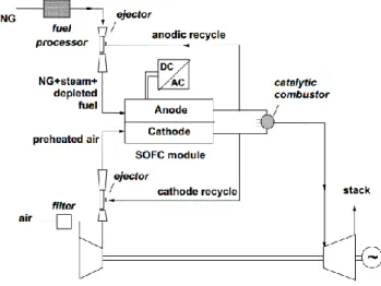
Supersonic ejectors can be used in SOFC [44], [45], [46] or MCFC [47], [48] cathodic and/or anodic recirculation lines (Figure 1-5) instead of fans or blowers (increasing system reliability) [3].
8
Anodic recirculation. High pressure fuel (primary flow) flows through the ejector, where the low pressure anodic exhaust (secondary flow) is entrained and mixes with the primary flow. The resulting mixed stream flows out the diffuser to at a higher pressure and then enters into the connected reformer [45].
According to Marsano et al [44], the functions of the ejector is recirculating the anodic gas to:
1. raise the secondary flow pressure to meet the FC pressure at the required level; 2. supply sufficient heat required for the reforming reactions in the reformer; 3. provide enough secondary flow rate to maintain a proper “Steam to Carbon
Ratio” (STCR) avoiding carbon deposition in the reformer and FC stacks. Cathodic recirculation. This ejector is used as an heat exchanger to pre-heat gas at cathode inlet [45].
A remark on SOFC/MCFC modeling. Since the cost of energy for fuel compression is remarkable [49], an extreme care should be taken in ejector design and an accurate model for evaluating both on-design and off-design ejector performances is required, but most of ejector existing models are developed for refrigeration applications.
These modeling approaches will cause large errors if used to model ejectors in SOFC systems due to the differences in geometries, working fluids properties and operating conditions [50]:
1. the diameter ratio of mixing chamber to nozzle throat is much bigger, due to the requirement of larger entrainment ratio;
2. primary and secondary flows are overheated gases instead of saturated vapors; 3. primary and secondary flows temperature and composition are different from
refrigeration ones;
4. pressure raise of the secondary flow is smaller than in refrigeration application.
1.3.2 Subsonic ejector applications in energy field
Subsonic ejectors are used in:
1. Proton Exchange Membrane Fuel Cell (PEMFC) based systems; 2. Chemical Looping Combustion (CLC) power plants.
1.3.2.1 PEMFC
PEM fuel cell is a subject of great interest because of its (i) high power density, (ii) low operating temperature and (iii) short start-up time [51].
The fuel, hydrogen, is usually stored highly pressurized, while the pressure of the fuel cell stack is relatively low; this high-pressure difference can be exploited by an ejector
9 that uses the high-pressure hydrogen as the primary fluid to entertain the anodic exhaust (Figure 1-6).
Figure 1-6 PEM based system studied by [25]
In PEMFC based systems, ejector is used to [25]:
1. utilize the pressure potential energy of hydrogen otherwise wasted; 2. recycle the unconsumed hydrogen to increase the fuel usage efficiency; 3. regulate the anode humidity with the recycle gas;
4. raise the secondary flow pressure to the level required by the cell.
PEM fuel cell must have a strictly control of water on electrodes [51]: in order to avoid condensation of water vapor (due to the low temperature of the primary and secondary flows) ejector has a convergent nozzle instead of a convergent–divergent one [25]: this is the main difference between ejectors used in PEM or in SOFC systems.
PEMFC based system (similar to the one in Figure 1-6) with an ejector on anodic recirculation line have been studied by [25], [52] and [53], whereas He et al. [54], [55] studied an hybrid fuel delivery system that consists of two supply and two recirculation lines (Figure 1-7).
10
The supply lines operate basing on the load demand: at low load demand, the supply line with a low pressure regulator mainly accounts for the supply of fuel, while at a high load demand the other line with a flow control valve is used to supply additional flow. An ejector and a blower is used to mix the exiting unconsumed fuel with the supplying flow through two recirculation lines.
1.3.2.2 CLC
Subsonic ejector are used in fixed bed CLC power plants [56] (Figure 1-8):
Figure 1-8 (a) ejectors used on both Air Reactor and Fuel Reactor lines [56] and (b) ejector used on Fuel Reactor line only.
Penati [56] used ejectors on both Air Reactor and Fuel Reactor (Figure 1-8a) recirculation lines. Ejectors function is recirculating Nitrogen and exhausts, providing enough to win reactors pressure loss (due to high temperature1
, a compressor cannot be used).
However due to high mass flow rate on Air Reactor, power plant efficiency gets worse if ejector performance is low: to overcome this problem ejector can be used only on Fuel Reactor recirculation line (Figure 1-8b).
1
11
Ejector modeling
Chapter 2
On the basis of governing equations, coupled with appropriate assumptions, it’s possible to build up models for studying ejector performance. In this this chapter is presented a review about single-phase ejector modeling, because this is by far the case where there is higher experience in modeling techniques: for this reason is possible to give guidelines for future studies. Two-phase flow ejector modeling is an interesting new field of study, but there is obviously less experience [22], [23]: a multi-phase approach requires, beyond competences in ejector modeling, not only a complete knowledge of two-phase flow behaviors but also a remarkable experience in Multiphase Computational Fluid Dynamics, which is a present field of study [57], [58].
2.1 Introduction to ejector modeling: models structure
Main steps in building a model are:1. choosing approach;
2. choosing fundamental hypothesis;
3. defining governing equation to be solved;
4. choosing auxiliary relations needed to close the governing equations. In following sections each of these points will be deeply examined.
2.1.1 Approach
There are two main ways of approaching ejector modeling [22], [23]:
1. thermodynamic modes. One-dimensional steady-state explicit equations are used to obtain state and parameters along the ejector. Detailed information such as shock interactions or turbulent mixing of two streams cannot be obtained by these models;
2. CFD models. Numerical methods are applied to solve the partial implicit differential governing equations, after being discretized using control volume techniques [59], [60].
2.1.2 Fundamental hypothesis of thermodynamic models
Due to the complexity of flow behavior (choking, shock and mixing of the two streams are too complicated to be modeled in a thermodynamic approach), some ideal assumptions are needed. On the other hand, some factors that do not influence the flow significantly can be neglected, reducing problem complexity.
12
Here is presented the list of basic assumptions common to every thermodynamic model: I. inner wall of the ejector is adiabatic: neglecting heat transfer between the ejector
and the environment, allows using isentropic relations;
II. flow inside the ejector is steady and isentropic: this hypothesis is based on assumption [I];
III. primary and secondary fluid are supplied to the ejector at zero velocity: inlet pressure and temperature are also equal to the total pressure and temperature; IV. velocity at the ejector outlet is neglected;
V. two fluids begin to mix with a uniform pressure at the mixing section.
2.1.3 Equations to be solved
Thermodynamic models are based on the following equations: 1. conservation of mass: ∑ ∑ (3.1) 2. conservation of momentum: ∑ ̇ ∑ ̇ (3.2) 3. conservation of energy; ∑ [ ̇ ( )] ∑ [ ̇ ( )] (3.3) CFD models are based on Navier-Stoker equations coupled with a turbulence modeling approach; due to the presence of a transonic flow, equations to be solved have to take into consideration both turbulence and compressibility (Figure 2-1 represents density contours at nozzle exit of a subsonic ejector: there is a remarkable density variation).
13 In a Reynolds-Averaged-Navier–Stokes (RANS) approach, the solver has to deal with Favre averaged Navier-Stokes equations [59] coupled with a RANS turbulence models:
{ ̅ ( ̅ ̃) ( ̅ ̃ ) ( ̅ ̃ ̃) ̅ [ ( ̃ )] [ ( ̅ ̅̅̅̅̅̅) ( ̅ ̅̅̅̅̅̅) ( ̅ ̅̅̅̅̅̅) ] ( ̅ ̃ ) ( ̅ ̃ ̃) ̅ [ ( ̃ )] [ ( ̅ ̅̅̅̅̅̅) ( ̅ ̅̅̅̅̅̅) ( ̅ ̅̅̅̅̅̅) ] ( ̅ ̃ ) ( ̅ ̃ ̃) ̅ [ ( ̃ )] [ ( ̅ ̅̅̅̅̅̅) ( ̅ ̅̅̅̅̅̅) ( ̅ ̅̅̅̅̅̅) ] ( ̅ ̃) ( ̅ ̃ ̃) ̅ [ ( ̃)] [ ( ̅ ̅̅̅̅̅̅̅) ( ̅ ̅̅̅̅̅̅̅) ( ̅ ̅̅̅̅̅̅̅) ]
2.1.4 Boundary conditions
Boundary conditions describe the behavior of the simulation at the edges of the control volume:
thermodynamic models common [23] use pressures at inlets and exit of the ejector. Also the mass flow rates [61] or the velocities of the primary and secondary fluids have been used as boundary conditions in some literatures;
CFD models common [23] use thermodynamics conditions at inlets (pressures and temperatures), pressure outlet [60] and no slip condition at walls.
2.1.5 Initial conditions
Some thermodynamic models need initial condition to start simulation, such as expansion ratio ⁄ [61], entrainment ratio ̇ ⁄ ̇ [62] or cross-section area of the constant-area throat tube [27]; CFD model need to be initialized and, due to the presence of multiple inlets (primary and secondary flow), it’s suggested an hybrid initialization [60].
2.1.6 Turbulence modeling
Turbulence has strong effect on the flowing process; CFD models use Boussinesq hypothesis [59], which brings to turbulence models based on an eddy viscosity assumption (Reynolds stress tensor is proportional to the mean deformation rate tensor):
̅̅̅̅̅̅ (
14
Thermodynamic models cannot model turbulence phenomena in detail: dissipation term is implemented by frictional and mixing losses, which are accounted by applying coefficients introduced in the governing equations [63] (section 2.3 for further details).
2.1.7 Auxiliary relations
Auxiliary relations involve state equation, and variable relations; first of all it’s important to define the kind of approach toward fluid, giving state equation:
( ) (3.5)
For an ideal gas it becomes:
(3.6)
Mach number is defined as:
⁄ (3.7)
Where c is the sonic velocity: √( )
; for an ideal gas it becomes:
√ (3.8)
A typical approach to thermodynamic ejector modeling uses the hypothesis of isentropic transformation [III], which gives the following equations (where –i is a generic ejector section):
1. mass flow rate per area unit:
̇
√ √(
)
( ) ( ⁄ )
(3.9)
2. area ratio between two sections:
( ) ( ) (3.10) 3. pressure ration between two section:
(
)
(3.11) Remembering the relations between static and total variables:
15 ( )
(3.12) and the following relation:
(3.13)
2.2 Thermodynamic ejector modeling: story and current
state-of-the-art
Thermodynamic models deal with global parameters: starting from a set of hypothesis (section 2.1.2), equations (section 2.1.3) and boundary conditions (section 2.1.4), they are able to provide global information on ejector, such as outlet conditions or the entertainment ratio ̇ ⁄ ̇ ; one of best examples of this global approach is given by Yu and Li works [64], [65] that are able to provide a very synthetic formulation for starting from assumptions, balance equations and boundary conditions:
√ ( )
( ) (3.14) In this section a review on thermodynamic modeling is provided, remarking the approach used in each study and advancement achieved from first works till nowadays.
2.2.1 A brief story on thermodynamic ejector modeling
Ejector modeling has been developed since first half ho the 20th century with reference to supersonic ejector, due to an increasing interest in steam jet refrigeration. In 1942 Keenan and Neumann [66] applied a one-dimensional analysis based on continuity, momentum and energy equations to predict ejectors performance under ideal gas assumption, but the difficulty in offering an analytical solution for the momentum equation, forced to use some experimental coefficients.
Later, in 1950 Keenan et al. presented a work [28] where two theoretical methods to approach ejector modeling were introduced, laying the fundamental models of one-dimensional ejectors design theory:
Constant Pressure Mixing (CPM) model: during mixing is supposed ;
Constant Area Mixing (CAM) model: during mixing is supposed . Keenan et al. [28] also demonstrated that the former ejector technology (CPM) has better performance, but the latter model (CAM) offers better agreement with
16
experimental results: for this reason, most of the mathematical models that followed are based on CPM ejectors.
Beside fundamental hypothesis pointed out in section 2.1.2, in [28] (i) were supposed that primary and secondary streams start mixing immediately after discharging from nozzles and (ii) no efficiencies were used to correct isentropic process:
1. the former assumption was overcome in 1977 by Munday and Bagster [29] who further developed the CPM model by assuming that (i) primary and secondary fluid start mixing in a section in suction/mixing chamber and that (ii) primary flow creates a converging duct for secondary flow;
2. the latter assumption was overtaken later in 1995 by Eames et al. [61] that modified Keenan’s model [28] to include irreversibility associated with the primary nozzle, mixing chamber and diffuser. This work is based on CPM theory but without considering Munday and Bagster [29] theory (in [61] it’s supposed that two streams mixed at the primary nozzle exit plane).
It’s important to remark that the works of Munday and Bagster [29] and Eames et al. [61] have given in the past and they give nowadays the basis of the approach in ejector modeling theory: a coupling between the theory proposed by Munday and Bagster [29] and the model proposed by Eames et al. [61] is presented in 1999 by Aly et al. [62]. However none of above models took in account secondary fluid chocking: to overcome this lack in 1999 Huang et al. [27] presented a double chocking model based on Munday and Bagster’s [29] theory. Obviously, a double chocking model have an increasing number of equations to consider secondary fluid choking.
All of the models considered above are based on ideal gas assumption: an improvement was given in 2000 by the work of Rodgaris and Alexis [67] who improved Munday and Bagster’s [29] model by using thermodynamic and transportation properties of real gas (using R717 as media); later, in 2001, Cizungu et al. [15] proposed one of the first studies to compare system performance with different working fluids. Others studies concerning real gas effects were published back till now:
2004. Selvaraju and Mani [68] used R134a, R152a, R290, R600a, R717;
2005. Yapici and Ersoy [69] used R123;
2006. Yu et al. [65] used R134a, R152a and R142b;
2007. Yu et al. [70] used R142b;
2012. Cardemil and Colle [71] used R141b, Steam, Carbon dioxide.
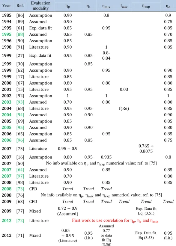
Once basis theory of ejector modeling was settled, the use of non-constant ejector efficiencies values was pointed out as main way to improve the accuracy of thermodynamic ejector models: their importance was already discussed in 1999 by Aly et al. [62], who found that efficiencies have a remarkable influence on system performance. In 2004 Selvaraju and Mani [68] proposed a model that uses an expression to describe the frictional loss in the constant area section (relating loss to
17 Reynolds number through friction factor in the form of the Darcy-Weisbach equation). Recently, in 2012, Liu et al. [72] proposed the first model using variable ejector efficiencies (estimated using empirical correlations retrieved from [73]). Further information on ejector efficiencies can be found in section 2.3.
General structure of approach presented in above studies (resulting from the coupling between the theory proposed by Munday and Bagster [29] and the model proposed by Eames et al. [61]) uses relations described in section 2.1.7 and models are organized in the following parts: (1) determining velocity and thermodynamic properties in the inlet of mixing section for both primary and secondary fluid; (2) using momentum equation to obtain condition of the outlet of mixing section; (3) using gas dynamics relations to study shock wave effects over Mach number and pressure; (6) determining velocity and thermodynamic conditions at diffuser outlet.
All of the models mentioned above gave only quantitative information, so Ouzanne e Aidoun in 2003 [74] proposed a local mathematical model based on Munday and Bagster’s [29] theory, isentropic flow and real gas (R142b): ejector is divided in control volumes and, for each of it, balance equations are solved; this model gives both qualitative and quantitative information on operation and performance of ejector. All works that have been presented above are based on the approach proposed in [29]: in 2007, Zhu et al. [75] developed a new approach to ejector modeling, proposing a model, called “Shock Circle Model” (SCM), which have been applied to an ejector operating in double-choking condition. Main features of this model are (i) the introduction of the “shock cycle” at the entrance of the mixing chamber (defined as the section where secondary fluid chokes) together with (ii) a 2D expression for velocity distribution to approximate the viscosity flow near the ejector inner wall:
1. shock circle (Figure 2-2): it’s assumed that for double-choking operating condition only the layer between primary and secondary flow is in the chocking condition and, being the layer very thin, it’s assumed that the layer sheet is a circle with zero thickness (which is defined as “shock circle”);
18
2. 2D velocity function (nomenclature from Figure 2-2) proposed in [75]:
{
( ) (3.15) Using logarithms, can be defined as:
( ) (
)
(3.16) In order to calculate , conditions at the “shock circle” are used: (i) the radius of the circle and (ii) the speed of sound at the shock circle:
{ √ (3.17) Hence: ( ) (√ ⁄ ) (3.18)
Once is known, secondary flow mean velocity and mass flow rate can be defined:
̅̅̅̅̅ ∫ ( ) (3.19) ̇ ∫ (3.20) Beside above consideration, general structure of this approach uses typical relations presented in section 2.1.7 and model is organized in the following parts: (1) determining the primary mass flow rate using isentropic flow relations; (2) determining velocity and thermodynamic properties in nozzle throat; (3) determining velocity and thermodynamic properties in the aerodynamic throat (4) approximating the velocity distribution of secondary flow by a 2D function; (5) deriving a simple formula for secondary mass flow rate; (5) establishing the energy conservation equation for primary and secondary flow.
19
refrigeration cycle with supersonic ejector operating in double-choking condition [75];
SOFC anodic recirculation with supersonic ejector operating in double-choking condition [50];
SOFC anodic recirculation, with supersonic ejector operating in: (i) back-flow, (ii) choking and (iii) double-choking condition [76];
Similar approaches, based on SCM, were developed for studying:
refrigeration cycle with or without steam condensation during flow expansion, with supersonic ejector operating in double-choking condition [77]2;
PEMFC anodic recirculation, with subsonic ejector [25], [55] 3;
Moreover SCM has been the basis for other models, such as the simplified ejector model for control and optimization presented in Zhu et al. [78].
Compared with a typical 1D model (such as the one proposed by Huang et. al. [27]) SMC model offers several advantages:
1. SCM is easy to run (there are less equation then standard 1D models in the solution procedure);
2. SCM can better predict ejector performance;
3. modeling of the mixing process in the constant area chamber is avoided;
4. only two basis coefficients ( and ) are used in SCM compared with 4 in the classical 1D models ( , , and ).
Last improvement in thermodynamic ejector modeling, as already remarked, is given by the proposal of a new approach (applied to a two-phase ejector) proposed in 2012 by the work Liu et al. [72], which is the first that develop a model using variable ejector efficiencies (estimated using empirical correlations retrieved from [73]).
In Table 2-1 a brief overview of relevant studies on thermodynamic modeling of single phase supersonic ejectors is presented.
Reference Working fluid Year, authors, work contributions and eventual presence of experimental data
[66] Air 1942. Keenan and Neumann. First paper to develop analytical model of ejectors. Experimental.
2 In this case there is not
, in fact it’s used a linear function for secondary flow velocity.
3
20
[28] Air 1950. Keenan et al. Fundamental work that laid the basis of CPM and CAM ejector modeling. Experimental.
[79] Air
1958. Fabri and Siestrunck. Fundamental study of ejector flow
phenomena; it introducesìd the idea of aerodynamic throat.
Experimental.
[29] Water
1977. Munday and Bagster. Fundamental work that further
developed Keenan theory [28] by considering that (i) primary and secondary fluid start mixing in a section in suction/mixing chamber and that (ii) primary flow creates a converging duct for secondary flow. Experimental.
[80] Air
1982. Dutton et al. They considered ejectors where secondary
stream enters at a supersonic velocity; mention of the effect of boundary layers on ejector operation. Experimental.
[81] Diatomic gas with
1986. Dutton and Carroll. Molecular weight was included as
optimization parameter; distinction between different operating regimes. Experimental.
[82] Ideal gas 1990. Sokolov and Hershgal. One of the first studies to consider working fluids other than air or water vapor. Experimental.
[61] Water 1995. Eames et al. One of the first works that used isentropic efficiency coefficients in order to take in account losses.
[62] Steam
1999. Aly et al. Coupling between the theory proposed by
Munday and Bagster [29] and the model proposed by Eames et al. [61] with considerations about ejectors efficiencies influences over system performance.
[27] R141b
1999. Huang et al. 1D model that supposed a constant-pressure
mixing occurring inside the constant-area section; experiments are used to calculate isentropic efficiency coefficients that include friction and mixing losses; coefficients used in many subsequent studies. Experimental.
[67] R717 2000. Rodgaris and Alexis. Improved Munday and Bagster’s [29] model by using real gas properties.
[15] R123, 134a, R152a, R717
2001. Cizungu et al. One of the first studies to compare
performance with different working fluids
21
both qualitative and quantitative information on operation and performance of ejectors (use NIST database for R141b) .
[68]
R134a, R152a, R290, R600, R717
2004. Selvaraju, and. Mani. First work to propose a
non-constant formulation of , related to friction loss in the
constant area section.
[69] R123 2005. Yapici and Ersoy, Local model for optimization of CAM ejector.
[65] R134a, 152a, R142b
2006. Yu et al. Best examples of global approach: provide a very
syntactical formulation for starting from balance equations, boundary conditions and assumptions (see equation 3.14).
[70] R142b
2007. Yu et al. Along with [65] is an important example of
global approach: provide a very syntactical formulation for starting from balance equations, boundary conditions and assumptions (see equation 3.14)
[75] R141b, R11
2007. Zhu et al. Develops model that is simpler than most 1D
models; takes into account radial velocity variation within mixing chamber from oblique shock
[50] Methane, Air
2007. Zhu et al. Uses model from Zhu et al. [75]; application in
SOFC anodic recirculation with ejector operating in double-choking condition.
[76] Methane, Air
2008. Zhu et al. Uses model from Zhu et al. [75]; SOFC
application in anodic recirculation, with ejector operating in: (i) back-flow, (ii) choking and (iii) double-choking condition [76]
[78]. Validated with R141b
2008. Zhu et al. Simplified ejector model for control and
optimization.
[83] R134a 2009. Guo and Shen. Model similar to Huang et al. [27]; gas property derived from NIST REFPROP.
[77] R141b, R11, steam
2009. Zhu et al. Uses model from Zhu et al. [75]; application in
refrigeration cycle with or without steam condensation during flow expansion, with ejector operating in double-choking condition
[71] R141b, Steam,
2012. Cardemil and Colle, The real gas equations of state are
22
[72]
2012. Liu et al. First model that uses variable efficiencies
estimated using empirical correlations, instead of being assumed to be constant value (two-phase flow ejector). Experimental. Table 2-1 Relevant studies about thermodynamic model for supersonic single phase ejectors
2.2.2 Subsonic ejector modeling: a recent theme of research
Subsonic ejector modeling is a recent theme of research and is linked to the growing interest in PEM fuel cell (section 1.3.2.2): the task of these models is to provide global parameters, such as outlet conditions or mass flow rate ( ̇ , ̇ ) flowing through the ejectors, for a given set of boundary conditions.
In this section, the models referring to literature presented in section 1.3.2.2 will be described; they all use different sets of equations to calculate ̇ and ̇ considering as working fluid and (PEM anode recirculating stream):
first models proposed in literature ( [52], [53] and [54]) used convergent nozzle equations;
Zhu and Li [25] proposed a model based on the same approach of Zhu et al [75], providing a more advanced model, which can simulate both a sub-critical and a critical ejector operating condition. This model has some constants that were calibrated using a CFD model;
He et al. [55] proposed an improvement of [25], providing a model that is able to simulate every operating condition of the ejector (back-flow, sub-critical and critical).
2006: 1D model proposed by Bao et al. [52]. Bao et al. in [52] used nozzle flow equations to calculate ̇ ; naming upstream pressure and downstream pressure , flow characteristic is divided into two regions by the critical pressure ratio: sonic (
) and subsonic flow (
). Using isentropic flow relations
and energy equation we can obtain:
for sonic flow:
̇ √
√ √ ( )
(3.21)
23 ̇ √ √ [( ) ( ) ] ( ) √ (3.22)
This model is able to take in consideration both critical and subcritical ejector operating condition (section 1.2.2).
2006: 1D model proposed by Karnik et Al [53]. Karnik et al. [53]studied a subsonic ejector using a 1D-CAM model:
primary flow ̇ through the ejector is obtained using the equation for choked flow through a nozzle:
̇
√ √ ( )
√ (3.23)
secondary flow ̇ depends upon the primary and secondary pressures :
̇ { ( ) √ √ ( ) √ (3.24) In these relations: 1. : nozzle throat;
2. : efficiency of the primary nozzle;
3. : efficiency for the secondary flow path (suction chamber); 4. : area of mixing tube;
5. : primary flow aerodynamic section determined supposing isentropic flow:
[ ( ) ] ( ) (3.25)
Where : is the coefficient that accounts for loss of primary flow affected at the boundary and is the Mach number of primary flow at the section where the secondary flow is choked:
[( )
( ) ] (3.26)
Obviously this model is unable to take in consideration subcritical ejector operating condition (section 1.2.2).
24
2008: 1D model proposed by He et al. [54]. He et al. in [54] used a 1D-CAP to build a model for a subsonic ejector with both primary and secondary streams operating in chocking condition:
• mass flow rate of the primary steam ̇ :
̇
√ √ ( )
√ (3.27)
• mass flow rate of the secondary steam ̇ :
̇ √ √ ( ) √ (3.28) In these relations: 1. : nozzle throat;
2. : efficiency of the primary nozzle;
6. : efficiency for the secondary flow path (suction chamber); 3. : area of mixing tube;
4. :the hypothetical throat area equal to the secondary flow section area where the flow is choked:
{
(3.29) Where is the primary flow section area determined by:
[ ( ) ] ( ) (3.30)
Where : is the coefficient that accounts for loss of primary flow affected at the boundary and is the Mach number of primary flow at the section where the secondary flow is choked:
[( )
( ) ] (3.31)
Obviously this model is unable to take in consideration subcritical ejector operating condition (section 1.2.2).
2009: 1D\2D model proposed by Zhu and Li et al. [25]. Li and Zhu in [25] presented a 1D\2D model that can simulate both a sub-critical (primary flow is subsonic) and a critical (primary flow is chocked) operating condition; due to the importance of this model, a detailed description has to be provided.
25 The following assumptions are made in developing the model:
1. the primary flow is treated as the ideal gas;
2. the primary and secondary flow velocity is uniform in the radial direction inside the ejector;
3. the velocity of the secondary flow inside the ejector is non-uniformly distributed in the radial direction;
4. pressure and temperature of both the primary and the secondary flows are uniformly distributed in the radial direction of ejector;
5. the isentropic relations hold in calculating friction losses using isentropic efficiencies.
Figure 2-3 Ejector studied by Zhu et al. [25]
Primary flow.
The flow through the convergent nozzle (between inlet and throat) is divided into two different regions: subsonic and sonic flow: due to the absence of a divergent part, the flow can only reach sonic flow condition when the pressure ratio is greater than the critical value (
)
.
Using isentropic flow relations and energy equation we can obtain (i) Mach number of nozzle throat of the primary flow and (ii) nozzle geometry :
sonic flow ( ): { ̇ √ √ ( ) √ (3.32) subsonic flow ( ):
26 { ̇ √ √ [( ) ( ) ] ( ) √ √ [ ( ) ] ( ) (3.33)
Where is the isentropic coefficient taking into account the flow friction loss.
Primary flow expands fully in the suction chamber: the pressure of the expansion flow can be represented by the secondary flow pressure . Using isentropic flow and energy balance laws for the primary flow from zone 1 to zone 2 can be determined:
1. Mach number: [ ( ) ] (3.29) 2. temperature: ( ) (3.30) 3. velocity: √ (3.31) 4. aerodynamic throat: [ ( ) ( ) ] ( ) ( ) (3.32) Where is a coefficient accounting for the frictional loss due to the mixing process.
Secondary flow.
Ejector performance is significantly affected by the flow characteristics in zone 2, where a mixing layer separates primary and secondary flows (which has a non-linear velocity distribution due to the turbulent flow and fluid viscosity as shown in Figure 2-4).
27 Figure 2-4 Radial velocity distribution in zone 2; taken from [25]
While in conventional 1D analysis, both velocities of the primary flow and secondary flow are treated uniform in the radial direction in [25] is proposed a 2D function:
{ ( ) (3.33) Based on this 2D velocity function and defining ⁄ the average density of the secondary, mean mass flow rate of secondary flow at Section 2 is:
̇ ∫ ( ) ∫ ( ) ( )( ) ( )( ) (3.34)
Remembering that ̇ ⁄ and ( ) mean velocity of secondary flow can be evaluated as:
( )
( )( )( ) (3.35) The velocity of the secondary flow is modeled by a 2D exponential function: this improvement led to a model which is capable of predicting the ejector performance within less uncertainties compared to the conventional 1D analysis [53], [52], [54]. Moreover, this treatment of the secondary flow velocity makes this model simpler than the conventional CAM or CAP theory: the model need only one algebraic equation for calculating ̇ .
![Figure 1-6 PEM based system studied by [25]](https://thumb-eu.123doks.com/thumbv2/123dokorg/7505527.104812/27.892.210.722.252.430/figure-pem-based-system-studied-by.webp)
![Table 2-5 Mixing efficiencies; taken from [63]](https://thumb-eu.123doks.com/thumbv2/123dokorg/7505527.104812/54.892.136.724.669.1040/table-mixing-efficiencies-taken-from.webp)
![Table 4-1 Operating conditions of tests performed by Gilbert and Hill [137]](https://thumb-eu.123doks.com/thumbv2/123dokorg/7505527.104812/78.892.146.723.192.493/table-operating-conditions-tests-performed-gilbert-hill.webp)
![Figure 4-4 Benchmark ejector; taken from [119].](https://thumb-eu.123doks.com/thumbv2/123dokorg/7505527.104812/80.892.240.617.541.820/figure-benchmark-ejector-taken-from.webp)
![Figure 4-18 Velocity profiles at (run 6) 050100150200250-1-0,50 0,5 1Velocity [m/s]](https://thumb-eu.123doks.com/thumbv2/123dokorg/7505527.104812/93.892.182.759.630.952/figure-velocity-profiles-run-velocity-m-s.webp)
