Near infrared diagnostics of Class 0/I protostars: the jets and accretion region

(1)

UNIVERSIT `

A DEGLI STUDI DI ROMA

“TOR VERGATA”

Facolt`a di Scienze Matematiche, Fisiche e Naturali

Dottorato Di Ricerca in Astronomia

XXI ciclo (2006-2008)

Near infrared diagnostics of Class 0/I

protostars: the jets and accretion region

Rebeca Garc´ıa L´opez

A.A. 2008/2009

Relatore esterno: Dott.ssa Brunella Nisini

Relatore interno: Prof. Roberto Buonanno

(2)

(3)

(4)

Abstract

In this thesis a study of the accretion and ejection properties of low mass embedded proto-star (the so-called Class 0/I sources) through ISAAC NIR high angular observations is pre-sented. The physics, kinematics and dynamics of five Class 0/I jets (HH1, HH111,HH212

/ HH34, HH46-47) have been analysed in order to give some insights about the jet

gener-ation and the dependence of the jet properties on the evolutionary stage of the source. In addition, the accretion properties of a sample of ten Class I sources have been measured in order to revise their evolutionary status.

All the studied jets have been observed through atomic and molecular emission, traced by [Fe ] and H2transitions. Applying near-IR diagnostic techniques important physical

parameters have been inferred. In particular, one milestone of this thesis was to derive the physical properties of embedded protostellar jets as a function of the jet radial velocity. For instance, at large distances from the source, the electron density (ne) has been found to decrease with lower velocities. Average values over the brightest knots of 2600-6200 cm−3

have been found. The amount of mass transported along the flows has been also inferred. The results show that Class 0/I jets transport more mass than the more evolved jets from CTTS, while the accretion to ejection ratio remains roughly constant independently of the evolutionary stage of the source.

The inner region of Class I jets has been studied in detail in order to constrain the jet launching mechanism. Similarly to what found in CTTS jets, Class I jets present two velocity components at high and low velocity (the HVC and LVC) in both the atomic and molecular gas. The LVC in Class I jets reaches, however, larger distances (up to

∼ 1000 AU from the source) with respect to jets from CTTS. At variance with what found at large distances from the source, in the inner jet region, ne increases with decreasing velocity, while the mass flux along the jet is always higher in the HVC. When comparing these results with the predictions of MHD jet launching models, the kinematical char-acteristics of the line emission are found to be, at least qualitatively, reproduced by the studied models. None of them can explain, however, the extent of the LVC and the veloc-ity dependence of electron densveloc-ity that is observed.

On the other hand, the study of the set of Class I sources reveals no clear correlation between accretion and ejection features. In addition, in spite of what is expected by embedded protostars, only four of the ten sources show accretion dominated luminosities. This result suggests that most of the objects considered as Class I sources are, instead, more evolved sources that have already acquired most of their mass. Despite this fact, the inferred mass accretion rates are larger that those found in CTTS of the same mass.

(5)

Sommario

In questa tesi viene presentata una analisi detagliata delle propietà di accrescimento ed eiezione da stelle giovanni estinte di basa massa attraverso osservazioni ad alta risoluzione angolare nel vicino infrarosso effettuate con la camera infrarossa ISAAC. In questo modo, sono state analizzate la fisica, cinematica e dinamica di 5 getti di Classe 0/I (HH1, HH111, HH212 / HH34, HH46-47) al fine di ricavare informazioni circa l’origine dei getti e la dipendenza delle loro propietà fisiche rispetto allo stadio evolutivo della sorgente. In-oltre, le propietà di accrescimento di un campione di dieci sorgenti di Classe I sono state misurate con lo scopo di acertare loro stadio evolutivo.

Tutti i getti studiati sono stati osservati per mezzo di emisione atomica e molecolare, traciate da righe di [Fe ] e H2. Applicando tecniche di daignostica nel vicino infrarosso,

sono stati ricavati importanti parametri fisici. In particolare, un punto fondamentale di questa tesi è stato derivare come varianno le propietà fisiche di questi oggetti in fun-zione della velocità radiale dello getto. Ad essempio, ne risulta che la densità elettronica decresce al diminuire della velocità a grande distanza dalla sorgente, con valori medi in-torno 2600-6200 cm−3_{. Inoltre, è stata ricavata la masa trasportata da i getti che risulta}

maggiore di quella trovata in oggetti pi`u evoluti di tipo TTauri, mentre il rapporto tra eiezione e accrescimento rimane approssimativamente costante indipendentemente dallo stato evolutivo dalla sorgente.

`

E stata altres`ı studiata in detaglio la regione interna dei getti di Classe I con il preciso fine di determinarne il mechanismo di lancio. Come per i getti da stelle di tipo TTauri, la cinematica delle regioni interne è caratterizzata da due componenti ad alta e bassa velocità (HVC and LVC) in entrambe le emissioni atomiche e molecolare. La componente a bassa velocità nei getti di Class I ragiunge distanze maggiori dalla sorgente (fino a 1000 AU) che nei getti di tipo TTauri. Inoltre, contrariamente a quanto trovato lontano dalla sorgente, nelle vicinanze della stella la densità elettronica aumenta al diminuire della velocità, mentre la componente ad alta velocità trasporta sempre la maggiore quantità di masa. I risultati qui mostrati sono stati inoltre confrontati con le predizione trovate dai modelli di lancio di getti. Mentre le propietà cinematiche sono, al meno qualitativamente, riprodotte da questi modelli, nessuno di loro riesce ad spiegare l’andamento osservato dalla densità elettronica in funzione della velocità.

D’altraparte, non è possibile stabilire alcuna correlazione tra la presenza di indica-tori di acrescimento ed egezione entro il campione di sorgenti di Classe I. Inoltre, di-versamente da ciò che previsto per le stelle giovanni, soltanto quatro delle dieci sorgenti hanno una luminosità dominata da accrescimento. Questo risultato sembra suggerire che

(6)

ii

la maggioranza di stelle giovanni clasificate come Classe I sono in realtà sorgenti molto più evolute che hanno già acquisito la maggior parte della loro massa. Nonostante ciò, i valori di tasa di accrescimento ottenuti sono in media più alti di quelli trovati in stelle di tipo TTauri della stessa masa.

(7)

List of Figures

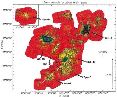
1.1 The ρ Ophiuchus molecular cloud complex mapped at 1.3 mm. Figure taken from Motte et al. (1998) . . . 2 1.2 Hertzsprung-Russel diagram for a sample of T Tauri and Herbig Ae/Be pre-main

se-quence stars (black points). The evolutionary tracks (Palla & Stahler 1993) for stars with masses M < 6 M⊙show the path of the stars from the birthline corresponding to

an accretion rate of 10−5M⊙/yr (bottom dotted line) to the Zero Age Main Sequence

(ZAMS, solid line on the left). The top dotted line is the birthline corresponding to ˙

Macc= 10−4M⊙/yr. The evolutionary tracks are almost vertical (Hayashi tracks) for

stel-lar masses smaller than 0.8M⊙, while the tracks relative to stellar masses between 2 and

6 M⊙(Herbig Ae/Be stars) are horizontal. The birthline intersects the ZAMS for M =

6 M⊙, thus the stars with larger masses have not a pre-main sequence phase. The thinner

solid lines are the isochrones for stellar ages of 105, 5×105, 106, 2×106, 5×106and 107 yr. . . 7

1.3 Schematic description of the various phases that characterise the formation of an indi-vidual star, from the earliest main accretion phase (Class 0), to the time when all the circumstellar matter is dissipated (Class III). The SED typical of objects in the various phases is represented on the left, while typical physical parameters of YSO according to their classification are listed on the right. . . 9 2.1 The interaction between the rotating magnetosphere of the central star and the

circum-stellar disc (Camenzind 1990). . . 12 2.2 Possible locations for the launching of MHD winds in young stars: disc-wind model

(upper panel, on the left), X-wind model (upper panel, on the right) and stellar wind (lower panel). In a disc-wind model, an extended magnetic field threads the disc, while in a X-wind model the magnetic field thread the disc through a singe annulus at the interaction point between the magnetosphere and the inner disc radio. When the field lines are anchored onto a rotating star we have a stellar wind. . . 13

(10)

iv

2.3 Left: the HH34 jet imaged by the VLT with the optical camera FORS2. Only the blue-shifted lobe of the jet is optically detected, while the red-blue-shifted lobe remains invisible as propagates inside the cloud. Both lobes terminate in a typical bow-shock structure. Right. The HH111 jet imaged at optical and near-IR wavelengths by Hubble Space Telescope. This jet presents a typical morphology with a chain of knots and a bow-shock at the head of the flow. Figures taken from ESO Press Release 17/99 (left) and Reipurth et al. (1997;right). . . 14 2.4 Spitzer image resulting from combining 3.6 µm(blue), 4.5+5.8 µm(green) and 24 µm(red)

images of the HH46-47 protostellar jet. A wide-angle outflow cavity is clearly seen to-gether with a compact jet propagating inside it. Two characteristic bow-shock structures are detected (HH47A and HH47C) corresponding to the end of the blue- and red-lobe of the outflow. Image taken from Velusamy et al. (2007). . . 15 2.5 Spectrum of the HH1 jet from 0.6 to 2.5 µm. Several atomic and molecular emission

lines are detected. Figure taken from Nisini et al. (2005b).. . . 16

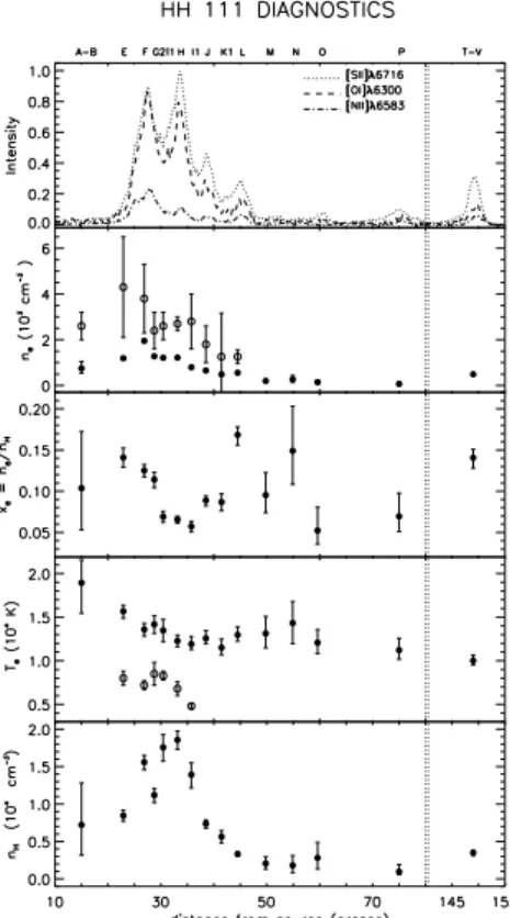
2.6 Variation of physical parameters along the HH111 jet. From top to bottom panel are represented: intensity profiles of the optical lines, the electron density, ne, in units of

103_cm−3_{, the ionisation fraction, x}

e, the electron temperature, Tein units of 104K and

the total density, nHin units of 104cm−3. The open circles are the values derived from

[Fe ] infrared lines, while filled circles represent values derived from [S ], [N ], [O ] optical lines. . . 17 2.7 Position-velocity diagram of the DG Tau jet, the archetype of CTTS jets. In the x-axis

the velocity of the jet is represented while in the y-axis the distance from the exciting source is indicated. In the diagram the intensity contours of the [O ] λ 6300 line are plotted decreasing by a factor of 2 beginning from a 83% of the peak. This jet exhibits typical kinematic features at the base, with a HVC that reaches far distances from the source and a LVC confined very close to the driving source. DG Tau is situated at a distance of ∼140 pc, thus 1′′ _{represents ∼140 AU. Figure adapted from Lavalley et al.}

(1997). . . 18 2.8 [Fe ] 1.644 µm predicted position-velocity diagram from the cold disc-wind model. In

the x-axis the velocity of the jet is represented while in the y-axis the distance from the exciting source is indicated. The model reproduces well the presence of an extended HVC and a LVC near the source. Figure adapted from Pesenti et al. (2004). . . 19 2.9 Position-velocity diagram of the SVS13, IRAS 04239, L1551, HH34 and HH72 jets near

the source through the H22.122 µm emission line. On the left panel the continuum of the

driving source has been subtracted leaving only the emission associated with the MHEL regions. The HVC and LVC have been indicated. Figure taken from Davis et al. (2001b). 20 2.10 Relation between the dereddened UV luminosity and the accretion luminosity for a

sam-ple of TTauri stars in the Taurus molecular cloud. Figure taken from Gullbring et al. (1998). 22 2.11 Relationships between the accretion luminosity and the luminosity of the Brγ and Paβ

lines for a sample of TTS in Taurus. Figure taken from Muzerolle et al. (1998). . . 23 2.12 Mass accretion rates derived from IR lines as a function of the stellar mass (M∗). Dots

and diamonds show ˙Maccvalues derived from the Paβ and Brγ line luminosities. Figure

(11)

LIST OF FIGURES v

3.1 Example of a NIR spectrum of the protostellar jet HH240. Several [Fe ] lines involving the first 13 levels of the Fe+and H2 emission lines are indicated. Figure taken from

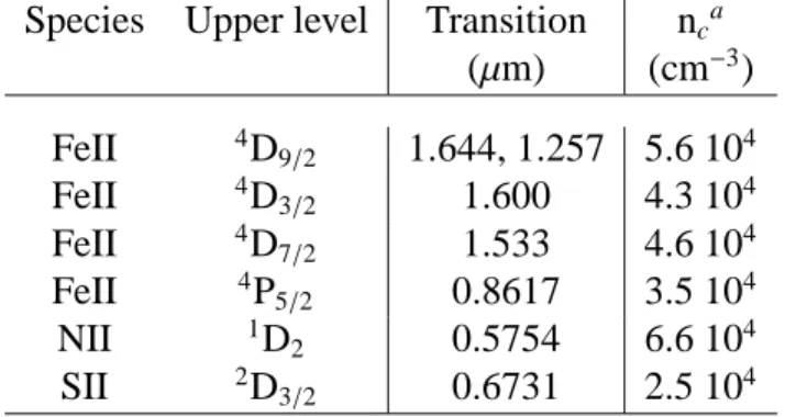
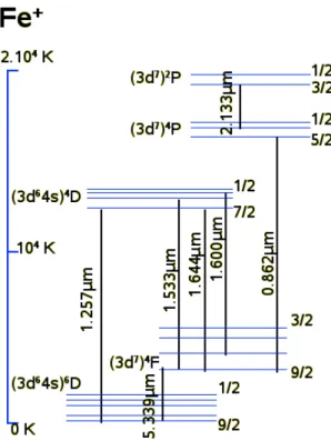
Nisini et al. (2002). . . 26 3.2 Fe+_{energy level diagram of the 16 first levels together with the (3d}7₎2_{P terms. The}

brightest transitions are indicated. . . 29 3.3 Theoretical ratio of the [Fe ] 1.533 and [Fe ] 1.644 µm lines calculated for different

electron temperatures (3 000,10 000, 20 000 K). Electron temperature increases from bottom to top. These transitions come from energy levels with similar excitation en-ergies thus their ratio is independent of electron temperature and then, very sensitive of electron density. Figure taken from Pesenti et al. (2003). . . 30 3.4 Diagnostic diagram based on [Fe ] lines. On the x-axis the [Fe ] 1.644/0.862 µm line

ratio (sensitive to Te) is represent, while in the y-axis the [Fe ] 1.644/1.533 µm line ratio

(sensitive to neis plotted. Dashed and solid lines indicates neand Tevalues of 103, 104

and 105_cm−3_{and 4, 5, 6, 8, 10, 15×10}3_{K. Figure taken from Nisini et al. (2005b).} _{. . .} ₃₁

3.5 Example of a Boltzmann diagram. When the gas is isothermal the value of ln(N(v, J)/gv,J)

for each line falls in a straight line which slope indicates the T_ex−1value. Different sym-bols represent lines coming from different vibrational levels. The 1-0S(1) and 1-0Q(3) lines have the same E(v, J) value, thus they can be used to estimate the visual extinction (see text). Figure adapted from Caratti o Garatti et al. (2006). . . 34 3.6 Example of a Boltzmann diagram for a thermalised gas. Different symbols indicate lines

coming from different vibrational levels. In this case, the value of ln(N(v, J)/gv,J) for

each line follow a curve. The dashed line represents the theoretical population distribu-tion of a gas at three different temperatures: 520, 2050 and 5200 K. Figure taken from Caratti o Garatti et al. (2008). . . 35 3.7 Sketch of a protostellar jet where the velocity (vt) and length (lt) of a section of the jet

perpendicular to the line of sight is represented. . . 36 4.1 Image of the HH1 jet taken by HST at four different wavelengths: NIR images in

[Fe ] 1.644 µm and H22.122 µm lines, and optical images in [S ] 0.6717/0.6731µm

and Hα lines. HH1 is a Class 0 protostellar jet, thus, a very embedded object. The

po-sition of the source, VLA1 (only detected at radio wavelengths), is indicated for all the panels. In the x- and y-axis the distance from the source is represented in arcseconds. The NIR lines trace regions closer to the driven source (down to ∼2′′_{) with respect to}

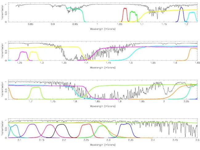
the optical ones that only trace gas down to ∼6′′ from the source. Figure taken from Reipurth et al. (2000a). . . 40 4.2 Model of the atmospheric transmission spectra of the J, H and K band for Paranal. The

response curve of the narrow band filters available at ISAAC are also plotted. In green is represented part of the Z filter and in yellow the J filter. The SH and H filters are indicated in magenta and blue, respectively, while, green and orange represent the SK and Ks filters. . . 41

(12)

vi

4.3 PVD for the H22.122 µm line along the HH111 jet (on the left). On the x-axis the

velocity with respect to the LSR is represented, while on the y-axis the distance from the source is reported. For comparison a narrow band H2image of the jet is presented

on the right. Figure taken from Davis et al. (2001a). . . 47 5.1 Three-colour composite image of the HH34 jet based on CCD frames taken with the

ESO instrument FORS2 at VLT. The composite was taken through three different filters: B (here rendered as blue), Hα(green) and [S ] (red). North is up and East is left. The

two bow-shocks HH34 N and HH34 S are indicated in the figure, together with the HH34 jet. Figure taken from Eso Press Release 17/99. . . 50 5.2 Continuum-subtracted K-band spectral images of the HH34 jet. Offsets in arcsec are

with respect to the HH34-IRS driving source. . . 51 5.3 Contours plot of the HH34 jet as seen in [S ] from the WFPC2 camera on HST. The

knots along the jet are identified. Figure taken from Reipurth et al. (2002). . . 53 5.4 Continuum-subtracted PV diagrams of the [Fe ] 1.644 µm and H21-0S(1) emission lines

for the blue and red lobe of the HH34 jet. A P.A. of -15◦ _{was adopted. Contours show}

[Fe ] 1.644 µm intensity values of 5, 15, 45, 135, 405 σ for the blue lobe, and 5, 10, 20, 40, 80 σ for the red lobe. The contours plotted on the H21-0S(1) PVDs show values of

5, 15, 45, 135, 405 σ for both lobes. On the Y-axis the distance from HH34 IRS is reported. 54 5.5 Continuum-subtracted PV diagrams for the [Fe ] 1.644 µm and H2 1-0S(1) emission

lines of the HH34 jet in the region nearest to the source. A P.A. of -15◦ was adopted. Contours show values of 5, 15, 45, 135, 260 σ for both lines. On the Y-axis the distance from HH34 IRS is reported. . . 57 5.6 Normalised line profiles (lower panels) of the [Fe ] lines 1.644 µm (solid line) and

1.600 µm (dotted line), and their ratio in each velocity channel (upper panel) for different extracted knots along the HH34 jet. Note that rA is a region that includes the knot rA. . 58 5.7 The electron density (upper panel) and mass flux (bottom panel) are represented as a

function of the distance from the source for the HH34 jet. Solid circles indicate the the electron density and mass flux for the HVC, while open circles refer to the values of the LVC. . . 60 5.8 HST image of the HH46-47 jet combining two WFPC2 images at [S ] and Hα

wave-lengths. Only the blue-shifted lobe of the jet is detected. The position of the source HH47 IRS is indicated together with some bright knots. North is up and East is left. . . 63 5.9 Position of the ISAAC slit superimposed on the H22.12 µm image of the HH46-47 jet.

Individual knots along the jet are identified following the nomenclature of Eisl¨offel & Mundt (1994). . . 65 5.10 LR spectrum from 1.00 to 2.50 µm of the knot Z1 in the HH46-47 jet. The stronger lines

are identified. . . 66 5.11 MR continuum subtracted spectral image of the HH46-47 jet in the K-band. . . 67 5.12 Continuum-subtracted PVDs for the [Fe ] 1.644 µm and H22.122 µm lines along the

HH46-47 jet. Contours show values of 3, 9, . . . , 243 σ for the [Fe ] line and 4.5, 13.5,. . . ,364.5 σ for the H2. On the Y axis distance from the source HH46-IRS in arcsec

(13)

LIST OF FIGURES vii

5.13 H2rotational diagram for the different lines in the knot Z1 of HH46-47. Different

sym-bols indicate lines coming from different vibrational levels. The straight line represents the best fit through the data. The corresponding temperature and the adopted extinction value is indicated. . . 71 5.14 Normalised line profiles (lower panels) of the [Fe ] lines 1.644 µm (solid line) and

1.600 µm (dotted line), and their ratio in each velocity channel (upper panels) for differ-ent extracted knots along the HH46-47 jet.. . . 72 5.15 HST image of the HH1 jet. (Top) NICMOS image in [Fe ] at 1.644 µm. (Bottom)

WFPC2 image in [S ] at 6717/6731 Å. The position of the source, VLA1, is indicated in both panels. Tick marks represents intervals of 1′′_{(∼460 pc at the distance of HH1).}

The detected knots along the flow are labelled. Figure taken from Reipurth et al. (2000a). 74 5.16 Continuum-subtracted K-band spectral image of the HH1 jet. Offset is with respect to

the CS star. . . 75 5.17 (left) Continuum-subtracted PVD for the H21-0 S(1) line along the HH1 jet. A position

angle of 145◦ _{was adopted. Contours show values of 10, 40, 60, 100 σ. On the Y-axis}

the distance from the driving source VLA1 is reported.(right) Normalised line profiles of the H21-0S(1) for different knots near the source. . . 77

5.18 Normalised line profiles (lower panels) of the [Fe ] lines 1.644 µm (solid line) and 1.600 µm (dotted line), and their ratio in each velocity channel (upper panel) for different extracted knots along the HH1 jet. . . 79 5.19 PV diagrams for the [Fe ] 1.64 µm, 2.13 µm and [Ti ] 2.16 µm emission lines of the

HH1 jet. A position angle of 145◦ _{was adopted. Contours show values of 11, 22,...,176 σ;}

4, 8, 12 σ and 3, 6, 12 σ, respectively. On the Y-axis the distance from the driving source VLA1 is reported. . . 81 5.20 HST mosaic image based on NICMOS and WFPC2 images of the HH111 jet. The

different knots along the jet are labelled. Figure adapted from Reipurth et al. (1999). . . 84 5.21 (left) PVD for the [Fe ] 1.644 µm line along the HH111 jet. A position angle of 22◦

was adopted. Contours show values of 5, 15, . . . , 405 σ. On the Y-axis the distance from the driving source HH111-VLA is reported. The velocity is expressed with respect to the LSR and corrected for a cloud velocity of 8.5 km s−1 _{(Davis et al. 2001a).(right)}

Normalised line profiles of the H22.122µm line for different knots along the jet. . . 85

5.22 Variation of the derived electron density along the HH111 jet. . . 86 5.23 Normalised line profile (lower panels) of the [Fe ] 1.600 µm line, and the [Fe ] 1.600/1.644 µm

line ratio in each velocity channel (upper panel) for different extracted knots along the HH111 jet. . . 87 5.24 (Left) ISAAC H2 image of the HH212 jet. North is up and left is East. The two insets

in the corners show the details of the inner jet region and a south-west bipolar nebula. Figure taken from McCaughrean et al. (2002). (Right) The H2image of the inner jet

where the knots have been labelled is shown together with the contours of the SiO (cen-tral panel) and CO (right panel) emission plotted on top of the H2 image. Figure taken

(14)

viii

5.25 PVDs for the H22.122 µm line along the blue-shifted (top) and red-shifted (bottom)

lobes of the HH212 jet. A position angle of 22◦ _{was adopted. Contours show values}

of 10, 30,. . . , 810 σ in both lobes. On the x-axis the distance from the central source is reported. . . 90 5.26 PVD for the [Fe ] 1.644 µm line along the HH212 jet. A position angle of 20◦ _was

adopted. Contours show values of 30, 60, 120 and 175 σ. . . 91 5.27 Normalised line profiles (lower panels) of the [Fe ] 1.644 µm (solid line) and 1.600 µm

(dotted line) lines, and their ratio in each velocity channel (upper panel) for different extracted knots along the HH212 jet. . . 92 5.28 PVDs of the [Fe ] 1.644 µm line for the HH34 and HH46-47 jets. . . 93 5.29 (left) Continuum-subtracted PVD of the [Fe ] 1.644 µm line for the RW Aur jet. The

[Fe ] emission features are indicated by dotted lines. Figure taken from Pyo et al. (2006). (right) Continuum-subtracted PVD of the [Fe ] 1.644 µm line for the HH34 jet. 94 5.30 (left) Predicted PVD of the [Fe ] 1.644 µm line from the cold disc-wind model,

assum-ing an inclination angle i=45◦. Figure taken from Pesenti et al. (2003). (right) Predicted PVD of the [S ] λ 6731 emission line from the X-wind model assuming an inclination angle of i=30◦_{. Figure adapted from from Shang et al. (1998).} _{. . . .} ₉₆

5.31 Comparison of predicted specific angular momentum vs. poloidal velocities for all types of stationary MHD models. Solid lines represent the relationship between rvφand vp:

in red for disc-winds assuming a fixed launching radius r0, in blue for stellar winds.

Dashed lines indicates curves of constant magnetic lever arm in the disc wind case. The position of the X-wind solution for a fixed r0= 0.07 AU is indicated by a thick red line.

Observational points for several TTauri jets are reported. . . 97 6.1 H- and K-band spectra of WL12. . . 102 6.2 J-, H- and K-band spectra of WL16. Both Brγ and Paβ lines show inverse P-Cygni profiles.103 6.3 (Top) J- and K-band spectra of GSS26. (Bottom) H- and K-band spectra of WL15. . . 104 6.4 J-, H- and K-band spectra of IRS54. . . 105 6.5 J-, H- and K-band spectra of WL17. . . 106 6.6 Mass accretion rate as a function of the stellar mass for the studied Class I sample

(aster-isks) and a set of CTTS and brown dwarfs (squares, crosses, plus and rhombi; Muzerolle et al. 2003; White & Ghez 2001; Gullbring et al. 1998; Calvet et al. 2004). . . 108 6.7 J-, H- and K-band spectra of WL18. . . 110 6.8 (Top)J-, H- and K-band spectra of YLW16A. (Bottom) H- and K-band spectra of YLW16B111 1 H2 rotational diagram for the different lines in the knot X1. Different symbols

indi-cate lines coming from different vibrational levels. The straight line represents the best fit through the data. The corresponding temperature is indicated. An extinction of AV=5.5 mag was adopted. . . III

2 H2 rotational diagram for the different lines in the knot X2. Different symbols

indi-cate lines coming from different vibrational levels. The straight line represents the best fit through the data. The corresponding temperature is indicated. An extinction of AV=7 mag was adopted. . . III

(15)

LIST OF FIGURES ix

3 H2 rotational diagram for the different lines in the knot X3. Different symbols

indi-cate lines coming from different vibrational levels. The straight line represents the best fit through the data. The corresponding temperature is indicated. An extinction of AV=8.5 mag was adopted.. . . I

4 H2rotational diagram for the different lines in the knot Y. Different symbols indicate

lines coming from different vibrational levels. The straight line represents the best fit through the data. The corresponding temperature is indicated. An extinction of AV=8 mag was adopted. . . I

(16)

(17)

List of Tables

3.1 Critical densities for the upper levels of some forbidden atomic lines. . . . 28

3.2 _{Radiative transition probabilities for [Fe ] lines taken from different} au-thors. . . 32

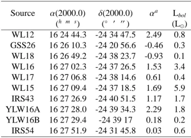
4.1 The observed sample: HH objects . . . 42

4.2 The observed sample: Class I sources . . . 43

4.3 Observations: HH objects . . . 44

4.4 Observations: Class I sources . . . 45

4.5 Wavelength range and nominal resolution for the J, SH and SK filters of ISAAC at LR for a 0.′′_{6 slit and at MR for a 0.}′′_{3 slit. . . .} ₄₆

5.1 List of detected lines . . . 52

5.2 Observed radial velocities along the HH34 jet. . . 56

5.3 M˙jet along the HH34 jet. . . 62

5.4 Lines observed in the knot Z1 of the HH46-47 jet. . . 64

5.5 Observed radial velocities along the HH46-47 jet. . . 69

5.6 AV along the HH46-47 jet. . . 69

5.7 T, ˙Mjet(H2) along the HH46-47 jet. . . 70

5.8 Electron density along the HH46-47 jet. . . 72

5.9 M˙jet along the HH46-47 jet. . . 73

5.10 List of detected lines . . . 76

5.11 Observed radial velocities along the HH1 jet. . . 78

5.12 M˙jet along the HH1 jet. . . 83

5.13 Kinematical and physical parameters of the HH111 jet internal knots . . . 86

5.14 List of detected lines along the HH212 jet . . . 90

5.15 Radial velocities along the HH212 jet. . . 91

5.16 M˙jet values along the HH212 jet. . . 92

5.17 Summary of the average physical properties in the considered sample of Class 0/I objects. . . 99

6.1 M˙accfor the observed targets. . . 107

6.2 Emission features in the observed Class I sources. . . 112 6.3 Observed unreddened lines along HH46-47: H2lines. . . I

(18)

xii

(19)

(20)

Introduction

The star formation process is a fundamental issue in stellar physics. It represents, how-ever, the less known process in the whole stellar evolution. This is mostly due to the difficulty of observing the protostars and the region nearby. Indeed, in the first stages of evolution, when most of the final stellar mass is accumulated, protostars are embedded in dense molecular clouds of gas and dust from which they originate. As a consequence, the younger protostars (the so-called Class 0 and I sources) are hidden to optical wavelengths and become only visible after they have dissipated most of their dense envelopes. This happens when they have overpassed their main accretion phase and are observed as pre-main sequence stars evolving towards the pre-main sequence (Class II and III sources). Only during the last twenty years, thanks to the development of infrared instrumentation, it has been possible to perform extensive studies on star forming regions.

Embedded protostars are very complex systems composed by a dense core surrounded by a circumstellar disc and a dense envelope, which represents the store of infalling ma-terial. As matter flows from the disc to the protostar surface part of the material is ejected away from the star in the form of collimated bipolar jets. These jets have a fundamental role in the star formation process, since they remove angular momentum from the star-disc system, allowing the accretion of matter onto the protostar to proceed. In addition, they influence the final mass of the star as they disrupt infalling material dissipating the surrounding envelope. Accretion and ejection of matter are thus intimately associated and represent the fundamental mechanism regulating the formation of a solar mass star.

In spite of their crucial role, the details of these processes are still largely unknown. Several models have been so far proposed for the mechanism regulating the accretion process and the consequent formation of the collimated jet. Most of these models have been developed to explain the properties derived from optical observations of Class II TTauri stars, sources that have already accumulated most of their final mass. Little is known, however, about the application of the same mechanism to the younger and actively accreting Class 0/I sources.

The main observational difficulty is to investigate the inner regions of the embedded Class 0/I sources at a spatial resolution high enough to resolve the relevant spatial scales. The accretion disc and the jet launching regions are, indeed, characterised by a size of the order of 0.1-1 AU, which corresponds to angular sizes of less than a few milliarcsec-onds even in the nearest star-forming clouds. Such angular scales can be directly probed only through IR interferometric techniques that at present are still under development. Alternatively, observational constraints to these phenomena can be provided only through

(21)

II

indirect tracers. In this respect, the study of the collimated jets provide a fundamental tool to get quantitative information on the active processes occurring in young stars. The jets extend up to large distances from their driving source, reaching regions at low obscuration where they can be studied in detail. As a consequence, the study of the jet often repre-sents the only mean to indirectly infer some properties of its driving source. Protostellar jets interact with the ambient medium producing strong shock waves which compress and heat the gas: this, in turn, cools down by emitting atomic and molecular lines over a large spread of wavelengths. The near IR spectral region is particularly suited to study the jets from embedded objects because several bright transitions excited in shocks can be found in this wavelength domain, able to diagnose important physical parameters of the jet. IR sensitive spectroscopic observations can, moreover, penetrate close to the jet base, thus providing information on the physics occurring as near as possible to the jet origin.

In addition to the study of jets, important information of the accretion process can be also inferred through the observations of spatially not resolved line emission features characterising the IR spectra of Class I objects. Permitted HI lines, in particular, are believed to originate from the region of accretion that connects the circumstellar disc to the protostar. Their luminosity and profiles provide therefore an important tool to investigate whether the protostar is still actively accreting or has already accumulated its final mass.

High dispersion IR spectroscopy performed on 8-m class telescopes provides an ex-cellent tool to perform the kind of investigations described above, since it couples the needed sensitivity and adequate spatial resolution with a spectral resolution high enough to study the dynamics of the matter in infall or being ejected from the source.

The work presented in this thesis aims at studying the accretion an ejection process in low mass embedded protostars (Class 0/I) through high resolution IR spectroscopy obtained with the ISAAC instrument at VLT. The work is divided in main parts whose goals are summarised below:

• The main part of this thesis deals with the detailed study of the physical and kine-matical properties of five classical Class 0/I jets. Long-slit ISAAC spectra have been obtained with the slit aligned along the jets in order to derive important pa-rameters as a function of the distance from the driving source. The IR investigation makes it possible to trace the jet very close to the central source. Thus, the excita-tion and dynamics of these jets have been probed as close as ∼100 AU from their origin in less embedded Class I sources, where their properties have not been yet modified by the interaction with the surrounding medium and still retain important information about the jet acceleration mechanism. Diagnostic techniques employ-ing ratios and luminosity of lines, e.g., [Fe ] and H2 transitions, have been used

to derive important physical parameters such as electron density (ne) and mass flux rates ( ˙Mjet) in the different jet velocity components. These parameters, together with the kinematical information, have been compared with the predictions of the-oretical models to constrain the jet launching mechanism. The physical properties derived in our Class 0 and I sample will be also compared with those of the jets from

(22)

Introduction III

more evolved CTTSs to understand if the excitation conditions and the dynamical properties change as a function of the source evolutionary state.

• The second part of the thesis address the accretion properties of a sample of ten Class I sources selected in the ρ Oph molecular cloud. The accretion properties and mass accretion rates of the sources have been measured from the luminosity of the permitted HI lines in order to investigate whether they are really sources in their main accretion phase or not. Indeed, it is usually assumed that the bolometric lumi-nosity of Class I objects is dominated by the accretion lumilumi-nosity due to the release of energy in the impact of the infalling matter onto the star surface. Should be this the case, we would expect that all the sources of our sample have a large Lacc/Lbol ratio. Mass accretion rates derived from the selected sources will be compared with the values measured in samples of TTauri stars to study if there is really an evo-lutionary sequence among Class I and Class II objects. This analysis will make it possible to discern whether the Class I are really younger than TTauri stars or they also are evolved objects but seen with edge-on circumstellar discs, thus appearing more embedded.

This thesis is structured as follows: In Chapter 1 a review of the star formation theory is presented, while in Chapter 2 a description of the present knowledge of the accretion an ejection properties of young stars is done, together with a brief description of the pro-posed models for these phenomena. In Chapter 3 the main diagnostic capabilities of IR emission lines are briefly described. The basic notions of IR spectra acquisition and anal-ysis techniques are presented in Chapter 4 together with a discussion on the advantages and limitations of IR observations and a description of our source sample and instrument set-up. In Chapter 5 the results on the ejection properties of Class 0/I jets are presented, while in Chapter 6 the findings on the accretion properties of the studied Class I sources are shown. Finally, conclusions are presented, summarising the main results of this work and describing future projects.

(23)

(24)

Chapter 1 The birth of stars

1.1 From molecular clouds to protostars

Most of the protostars are born inside Giant Molecular Clouds (GMCs). These are the largest molecular structures in the galaxy with sizes ranging between 10 and 100 parsec (pc), masses from 104 _{to 10}6_M

⊙ and average kinetic energies of only ∼10 K. Their

prin-cipal chemical components are hydrogen (90%) and helium (9%), while the abundance of other elements depends mainly on the history of the cloud as, for example, the pres-ence of some supernova explosion nearby. GMCs are far to be uniform with the dust and gas distributed along very complex and filamentary structures with areas of high density corresponding to star formation regions. Most of the information we have about GMCs is derived through the analysis of emission lines coming from rovibrational transitions of CO, CS or NH3molecules. Although the main constituent is H2, molecular clouds cannot

be mapped through this molecule due to the high temperatures (∼510 K) required to excite detectable emission. The best tracer of the molecular cloud structure is the CO molecule since is quite abundant ([CO]/H2∼10−4) and can be easily populated under collisions at

low temperatures (T∼ 5 K with n(H2 >100 cm−3)). In addition, the CO dissociation

en-ergy is very high (11.09 eV) meaning that is a very stable molecule. The CO emission in our galaxy is located mainly in the spiral arms suggesting that GMCs have lifetimes of the order of 107_{years. The larger is the molecular cloud the shorter is its lifetime. This is}

due to the photoevaporation produced by O and B stars that form inside large molecular clouds. These stars produce high energy photons that ionise and destroy their molecular surroundings.

The complicated density structure of GMCs (Fig. 1.1) can be roughly classified in terms of clouds, clumps and pre-stellar cores (Williams et al. 2000). Clumps are gravi-tationally bound structures inside which stellar clusters are formed. Pre-stellar cores are the smallest fragments out of which individual stars or multiple systems are born. These initially gravitationally bound condensations form from the fragmentation of molecular clumps. A large number of pre-stellar cores have now been observed, both in molecular line tracers of dense gas such as NH3, CS, N2H+ and HCO+ (Andre et al. 2000) and in

(25)

2

Figure 1.1:The ρ Ophiuchus molecular cloud complex mapped at 1.3 mm. Figure taken from Motte et al. (1998)

There is yet not a complete understanding of how stars are born from dense cores. A core begins to collapse when the thermal pressure of the gas within the core is no longer sufficient to contrast self-gravity. This means, in the classical theory proposed by Jeans (Jeans 1902), that collapse occurs when the gravitational energy of the cloud core is greater than its thermal energy,

|Eg|> Eth (1.1)

which, for a homogeneous spherical core with mass M, radius R and temperature T, is given by: 3 5 GM R > 3 2 M µmH kT (1.2)

where G is the gravitational constant, k the Boltzmann constant, µ the mean molecular weight and mH the mass of the hydrogen atom. This inequality is, usually, expressed in terms of the Jeans mass MJ: gravitational collapse begins when the core mass M is greater than MJ, M > MJ = 3 4πρ !1/2 5kT 2GµmH !3/2 ≃ 6M⊙ T3 n !1/2 (1.3) where ρ is the density of the gas and n = ρ/µmHis the numerical density.

In absence of pressure support, the collapse due to gravitation occurs in a free-fall time: tf f = 3π 32Gρ !1/2 ≃1.4 × 106 n 103_[cm−3_] ! [yr] (1.4)

(26)

The birth of stars 3

If T =10 K and n ≥50 cm−3_{, which are typical values for GMCs, we have M}

J ≃100 M⊙and

tf f ≃105yr. These values are smaller than the observed values of mass (104-106M⊙) and

lifetime (>107_{yr) of the clouds. Thus, on the basis of the classical theory, molecular}

clouds should be small short-lived structures with a star formation rate of about 250-300 M⊙yr−1, while observations indicate rates of only 3 M⊙yr−1.

The Jeans criterion is thus unable to describe observational data, providing only a necessary and not sufficient condition to have an unavoidable collapse. Other mechanisms capable of hampering and delaying gravitational contraction must be, therefore, present within the clouds.

Nowadays, three physical mechanisms are believed to concur with the thermal pres-sure in supporting the core against self-gravity: magnetic field, core rotation and gas turbulence. Thus, the most general condition to be satisfied is:

|Eg|>Eth+ Emag+ Eturb+ Erot, (1.5) where Eth is the thermal energy due to gas pressure, Emag is the magnetic energy due to magnetic pressure and Eturband Erotare the terms due to turbulence and rotational velocity of the clumps, respectively. We will now briefly describe these terms:

• Rotation: From measurements of the rotational velocity by means of the study of

Doppler shifts in lines from molecular species, we know that the cores rotate very slowly (Ω ∼ 10−13 − 10−14 rad/s, Goodman et al. 1993). Therefore, Erot can be neglected if we compare it with the pressure gradients and the self-gravity. This rotation play a fundamental role, however in the formation of protostellar disc as we will see in Sect. 1.2.

• Magnetic field: The presence of a magnetic field B (usually smaller than 10 µG

in molecular clouds and up to 50 µG in the cores) provides support against gravita-tional collapse because the ions present in the cloud gas tend to couple with the mag-netic field lines. Moreover, neutral constituents are affected by this phenomenon, since collisions couple ions with neutrals, resulting in an overall magnetic pressure which halts and slows down gravitational contraction. Assuming that the magnetic energy is the only term capable to compensate the gravitational energy of the cloud in eq. 1.5, the criterion for core collapse can be expressed in terms of critical mag-netic mass Mφ: M > Mφ≃ 0.3G−1/2B R2 = 200M⊙ B 3[µG] ! R 1[pc] !2 (1.6) If the cloud mass M exceeds Mφ, the cloud globally implodes forming stars: this

is the case of high mass stars in magnetically supercritical cloud cores (M ≫ Mφ),

where the collapse takes place in a free-fall time-scale tf f. Otherwise, the forma-tion of low mass stars occurs in magnetically subcritical cloud cores (M ≪ Mφ),

that are quasi-static equilibrium structures resulting from the balance of gravita-tional, magnetic and pressure forces. The core collapse in these systems occurs

(27)

4

because of a process called “ambipolar diffusion”: since ions and neutrals are not strongly coupled, the neutrals can drift across the field lines resulting in a gravi-tational condensation of the cloud matter without compressing the magnetic field lines. Truly neutral drift motion deforms the magnetic field lines, producing Alfv´en waves that dissipate the magnetic field. As a result, ambipolar diffusion produces the effect of decreasing the critical magnetic mass, so that the core can collapse when M ≫ Mφin a time-scale (ambipolar diffusion time tAD) that depends on the efficiency of the coupling between ions and neutrals. For typical values of molecu-lar cores tAD ∼5×106yr, one order longer than the free-fall tf f.

Magnetic diffusion was believed to be the dominant physical process controlling star formation and it was widely accepted in the 80s. During the last decade, with the improvement in instrumentation and computer modelling techniques, this theory has seemed, however, to fail on some aspects, although the debate is still open. Indeed, observations seem to suggest that protostellar cores are supercritical (i.e. the magnetic fields are too week to retard the gravitational collapse of cores) and infall motions detected in the cores contradict the long lasting phase that is expected in the standard theory. Finally, a high fraction of cores which contain embedded protostellar objects is observed: if cores evolved on ambipolar diffusion time-scales, we would expect to find a significantly larger number of starless cores.

• Supersonic turbulence: During the last decade, substantial observational evidence

suggests that supersonic turbulence is the main process controlling star formation. The random supersonic motion in molecular clouds is described by the Mach num-ber M = vturb/cs, where vturb =

p

hv2_i_{is the average speed of the random motions}

and csis the sound speed. The observational evidence of this motion comes from velocity dispersion measurements of molecular line widths of 4-6 km s−1_{, that}

can-not be accounted for unless considering non-thermal motions.

Turbulent supersonic motion is a dissipative phenomenon able to reallocate energy inside the cloud, providing a global support against gravitational collapse. The dissipation time for turbulent kinetic energy is indeed:

td= Ld vturb = 3 Myr Ld 50[pc] ! vturb 6[kms−1_] !−1 (1.7)

where Ld is the driving scale of the turbulence. Numerical methods and computer simulations demonstrate that supersonic turbulence within large clouds would dis-sipate in a time-scale which is comparable to the free-fall time-scale. A recurring injection of energy is, then, needed to maintain turbulence as long as is necessary to obtain the observed core contraction times. Several mechanisms have been consid-ered, such as galactic rotation, MHD wave propagation, protostellar outflows and, in particular, supernova explosions.

(28)

1.2 The evolution of Young Stellar Objects (YSOs)

As described above, low-mass star formation is thought to occur when a molecular cloud core becomes unstable and begins to collapse. During the last years, several studies have been done trying to measure the infalling motions gas within the cloud core. However, the detection of these motions are very difficult. The velocities of collapse are too small if we compare them with the random motions inside the molecular cloud. This fact becomes extreme if we try to distinguish the infall motion against fast molecular gas put in motion by bipolar outflows (see Sect. 2.1). On top of all this, the highest velocities are expected to be present in the central regions of the cloud, where, however, the amount of mass is really low and the extinction is very high.

Despite the lack of measurements of infalling velocities, some theoretical models have been developed in order to give some light about the very first phases of the stellar evo-lution. One of the simplest models assumes that the molecular core about to collapse presents a density profile ρ ∝ R−2 _{(singular isothermal sphere in quasi-equilibrium}

be-tween thermal pressure and gravity). When the structure becomes gravitationally unsta-ble, the collapse starts, following the free-fall time-scale. Being τf f ∝ ρ−1/2, the central zones collapse more rapidly than the outer part. As a result, at the centre of the structure a core in hydrostatic equilibrium is formed, which accretes matter from the surrounding infalling envelope. In this simple infall model, with an initial cloud spherically symmet-ric that exhibits asymmetsymmet-ric rotation, the infall solution has complete symmetry above and below the equatorial plane. With this assumption, the momentum fluxes of infalling material on either side of the equatorial disc plane perpendicular to the disc are equal in magnitude and opposite in direction. The result is that the infalling gas must pass through a shock at the equator, which cancels the kinetic energy component perpendicular to it. This process will lead to an accumulation of matter in a thin structure in the equatorial plane, i.e., a rotating disc. Ultimately, disc material will be redistributed by the process of angular momentum transport and energy loss driving disc accretion. The accretion rate depends on the sound speed in the medium (cs= (kT/µmH)1/2):

dM dT ≡ ˙Macc = ρ4πR 2 cs= 2 c3 s G (1.8)

For typical values, accretion rates of ∼10−5_-10−6_M

⊙yr−1 are derived. In this way, the

time expected for the formation of a solar mass star is around 106 years. In this phase, there are no nuclear reactions in the star and the luminosity of the YSO comes from the energy realised during the accretion in the so called “accretion shocks”. Assuming a spherical geometry for the accretion, the luminosity emitted is given by the conversion of gravitational energy:

Lacc =

GM∗M˙acc R∗

(1.9) where M∗and R∗are the mass and radius of the central condensation. For a typical values

of low-mass protostars (M∗= 1 M⊙, R∗ = 4 R⊙ and ˙Macc = 10−5M⊙/yr) the accretion luminosity is around 50 L⊙, much higher than the luminosity of a main sequence star with

(29)

6

the same mass. It has been observed that the accretion process is usually accompanied by the ejection of material from the protostar. This is the origin of the so-called protostellar jets, the main topic of this thesis and described in detail in the following sections.

In the early stage of evolution, protostars have a low surface temperature (T < 2000 K) and thus emit most of their energy at IR wavelengths. In addition, the emitted radiation is absorbed by the external envelope and re-emitted at longer wavelengths. This means, that in the protostellar phase the YSO is not simply characterised by a single temperature and thus cannot be positioned in the Hertzsprung-Russel (HR) diagram. When the gravi-tational collapse finishes and the envelope has been dissipated, the YSO becomes visible at optical wavelengths and can be positioned in the HR diagram. This is the so-called pre-main sequence phase (see Fig. 1.2). At this stage, the star has almost reached its final mass and the accretion rate is very small, around 10−7M⊙/yr. In the pre-main sequence

phase the central temperature of the stellar core is still too low to permit the hydrogen fusion into helium. Deuterium fusion occurs at temperatures lower than hydrogen fusion, but since deuterium abundance is relatively low, the deuterium fusion can last only for a short period of time (∼ 1 × 10−6_{yr). Without fusion energy release, the protostar must}

contract, generating gravitational potential energy to replace the energy lost by the radi-ation of the stellar photosphere. Thus, the luminosity is mainly the energy irradiated by the stellar photosphere:

L∗= 4πR2σT_{e f f}4 (1.10)

where σ is the Stephen-Boltzmann constant and Te f f is the temperature of the stellar pho-tosphere. When protostars appear for the first time on the HR diagram, they are located along the so-called “birthline”, whose position in the HR diagram depends on the proto-stellar accretion rate. While the protostar contracts (typical time-scale of 107_{yr), it moves}

in the HR diagram along the pre-main sequence tracks. The contraction will stop when the star arrives in the main-sequence, at which point the energy released by the hydrogen fusion compensate the energy radiated by the stellar photosphere.

The low-mass (M . 2 M⊙) pre-main sequence stars, with stellar spectral types F-M are

called T Tauri stars (Joy 1945). These stars are fully convective and follow the so-called Hayashi tracks, along which the temperature is roughly constant, while the luminosity decreases with the radius. Higher-mass (M ∼2-10 M⊙) pre-main sequence stars are named

Herbig Ae/Be stars (Herbig 1960) to distinguish them from other types of more evolved A-B emission line stars. These stars have, at variance with TTauri, radiative nuclei and follow evolutionary tracks nearly horizontal (see Fig. 1.2).

1.3 The Spectral Energy Distribution classification of YSOs

The evolutionary status of a “normal”, low-mass star can be determined by its position on the HR diagram (see previous section). This method works as far as the star produces a black-body like spectrum and thus can be accurately spectrally classified. This is, how-ever, very difficult for most of the YSOs. The circumstellar gas and dust around these objects absorb and reprocess most of the radiation emitted by the embedded star, thus

(30)

Figure 1.2: Hertzsprung-Russel diagram for a sample of T Tauri and Herbig Ae/Be pre-main sequence stars (black points). The evolutionary tracks (Palla & Stahler 1993) for stars with masses M < 6 M⊙show

the path of the stars from the birthline corresponding to an accretion rate of 10−5_M

⊙/yr (bottom dotted

line) to the Zero Age Main Sequence (ZAMS, solid line on the left). The top dotted line is the birthline corresponding to ˙Macc= 10−4M⊙/yr. The evolutionary tracks are almost vertical (Hayashi tracks) for stellar

masses smaller than 0.8M⊙, while the tracks relative to stellar masses between 2 and 6 M⊙(Herbig Ae/Be

stars) are horizontal. The birthline intersects the ZAMS for M = 6 M⊙, thus the stars with larger masses have

not a pre-main sequence phase. The thinner solid lines are the isochrones for stellar ages of 105, 5×105, 106, 2×106, 5×106and 107yr.

(31)

8

altering its spectral appearance. In fact, the youngest objects are not detected at optical wavelengths due to the presence of a thick protostellar disc and a dense envelope that radiate most of their energy in the IR. In addition, in their first evolutionary stages, the circumstellar gas and envelopes have spatial extent larger than the protostar photosphere itself and thus, the YSO will exhibit a wide range of effective temperatures. As a result, the detected spectral distribution is much wider than a simple black-body spectrum. For all these reasons to place a YSO on a HR diagram is very difficult.

Lada (1987) found that the infrared sources could be classified as a function of their IR energy distributions (i.e., log(λFλ) vs. log(λ)). The shape of the broad-band IR spectrum

of a YSO depends both on the nature and distribution of the surrounding material. We would expect that more embedded objects show a spectral distribution with a black-body profile at the dense envelope temperature, while more evolved objects should have a spec-tral distribution characterised by the black-body emission of the censpec-tral protostar (since they should be accreted most of their surrounding material). In this way, the spectral energy distribution (SED) of a YSO can give some clues about its evolutionary status.

Lada & Wilking (1984) classified the YSOs as a function of their SED from Class I to Class III objects. With the pass of the years it was necessary to include a new type of colder objects, the Class 0 objects (Andre et al. 1993). This first stage (see Fig. 1.3) corre-sponds to a very embedded protostar, where the mass of the central core is small in com-parison to the mass of the accreting envelope. The SED of these objects is characterised by the blackbody emission of the envelope and peaks at sub-millimeter wavelengths. The accretion rate of Class 0 objects is very high, of the order of ˙Macc∼10−4M⊙/yr. The next stage is represented by the Class I objects. They are poor evolved embedded stars with less mass in the envelope and more massive central cores with respect to the Class 0 ob-jects. Their SED peaks in the far-infrared and is characterised by a weak contribution of the blackbody of the central star (detected at near-IR wavelengths) and the emission of a thick disc and dense envelope. The accretion rate is lower than in Class 0 objects with a typical value of the order of ˙Macc∼10−6M⊙/yr. Class II objects are the classical T Tauri stars (CTTS) with a SED due to the emission of a thin disc and the central star. They have accumulated most of their final mass, dispersed quite completely their circumstellar envelope, but still accreting at a very low rate of the order of ˙Macc∼ 10−7-10−8M⊙/yr. Fi-nally, Class III objects have pure photospheric spectra. Their SED is peaked in the optical and is well approximated by a blackbody emission with a faint infrared excess due to the presence of a residual optically thin disc that may be the origin of planetesimals.

This classification scheme can be made more quantitative by defining the spectral index:

α = dln(λFλ

dln(λ) (1.11)

defining the slope of the spectrum between 2 and 12 µm . α varies from 0 to +3 for Class I objects, -2 < α < 0 in Class II objects and for Class III objects it ranges from -3 to -2. This variation in SED shape represents an evolutionary sequence corresponding to the gradual dissipation of gas and dust envelopes around young stars. Adams et al. (1987) were able to theoretically model this empirical sequence from protostar to young main

(32)

Figure 1.3: Schematic description of the various phases that characterise the formation of an individual star, from the earliest main accretion phase (Class 0), to the time when all the circumstellar matter is dissipated (Class III). The SED typical of objects in the various phases is represented on the left, while typical physical parameters of YSO according to their classification are listed on the right.

(33)

10

sequence stars.

Today this classification must be applied with some caution. Although the general scheme is probably correct, recent observations have lead to some doubts about the ex-istence of real physical differences between many Class I and II objects. Geometrical effects due to the orientation of the structures with respect to the observing line of sight may alter the shape of the SED causing a misclassification of the objects. This issue will be addressed in the second part of this thesis (Chap. 6).

(34)

Chapter 2 Ejection and accretion of material in

low-mass YSOs

Accretion and ejection of matter are two phenomena intimately related during the forma-tion of a star. This thesis reports an observaforma-tional study of the ejecforma-tion, through collimated jets, and accretion of matter in young embedded Class 0/I protostars. To put the presented work in a context, I will make here an overview of the present knowledge of the accretion an ejection properties of young stars, presenting also a brief description of the proposed models for these phenomena.

The Chapter is divided in two main sections dealing with jets (Sect. 2.1) and accretion properties of YSOs (Sect. 2.2).

The discussion about protostellar jets is subdivided into a summary of the main ejec-tion models (Sect. 2.1.1), an overview of the large scale observaejec-tional characteristics (Sect. 2.1.2) and a description of the physical properties found at the base of protostel-lar jets (Sect. 2.1.3).

Finally in Sects. 2.2.1 and 2.2.2 the accretion characteristics of CTTS and Class I sources are discussed separately.

2.1 Protostellar jets

The evolution from Class 0 to Class III requires the dissipation of the circumstellar mate-rial in the protostellar infalling envelope and in the disc. In principle, this could be done by accreting all the surrounding material onto the star. We know, however, that star form-ing cores contain more mass than the stars themselves. This suggests that at some point in the early evolution of a YSO the cloud material has been partially removed. In addition, the mass accretion process needs to be followed by the dissipation of angular momentum. In fact, to conserve angular momentum the star would be forced to rotate at increasing velocities leading to its break-up.

As noted in the previous chapter, the accretion process is associated with ejection of material from the star in form of energetic bipolar outflows since the first stages of

(35)

proto-12

Figure 2.1: The interaction between the rotating magnetosphere of the central star and the circumstellar disc (Camenzind 1990).

stellar evolution . These supersonic and collimated jets significantly contribute at both the angular momentum removal and envelope dissipation. In fact, recent observations seem to indicate that protostellar jets rotate (Bacciotti et al. 2002; Coffey et al. 2004), suggesting that they can efficiently contribute to the remove of angular momentum from the system (Ferreira & Casse 2004), helping to spin-down the protostar (Ferreira et al. 2006) and al-lowing the accretion of material. In addition, as protostellar jets propagate supersonically through the molecular cloud, they disrupt infalling material from the collapsing cloud influencing the final mass of the protostar (Terebey et al. 1984). Protostellar jets have therefore a fundamental role in the star formation process, although the exact mechanism for their formation is still unclear.

In this section, the basics of theoretical models so far developed for the jet launching are presented, together with a general description of their physical properties as derived from observations.

2.1.1 The launching mechanism

Theoretical models for accretion and ejection of matter in YSOs have as a common ele-ment the influence of the magnetic field. The magnetic field structure in the inner regions of the star-disc system is believed to acquire a configuration like the one in Fig. 2.1. A magnetised star with a dipolar field configuration accretes material from a disc through the magnetic field lines. The magnetic field of the protostar is believed to be strong enough to truncate the disc at a few stellar radii from the star (the truncation radius or

(36)

magne-Ejection and accretion of material in low-mass YSOs 13

Figure 2.2: Possible locations for the launching of MHD winds in young stars: disc-wind model (upper panel, on the left), X-wind model (upper panel, on the right) and stellar wind (lower panel). In a disc-wind model, an extended magnetic field threads the disc, while in a X-wind model the magnetic field thread the disc through a singe annulus at the interaction point between the magnetosphere and the inner disc radio. When the field lines are anchored onto a rotating star we have a stellar wind.

topause) and creates a magnetospheric cavity as shown in the Fig. 2.1. Very briefly, the accretion process is supposed to occur as follows. The material from the outer parts of the disc spirals toward the inner disc region. At this point, if the material is ionised enough it will be forced to move longward the magnetic field lines to partially accrete onto the pro-tostar and partially be ejected in a wind. When the material reaches the propro-tostar surface, through the so-called accretion-columns, it produces strong accretion shocks that create hot spots on the star surface. There are several observational evidences for the presence of such hot spots on the surface of accreting protostars (see e.g. Bouvier et al. 1995).

The accretion is only possible if the truncation radius is smaller than the corotation radius (RCO). The corotation radius is the radial distance at which the keplerian velocity of the material of the disc equals the stellar angular velocity. Outside the RCO, the angular velocity of the star is larger than the keplerian velocity. Thus, the material along the field lines of the magnetosphere is thrown away due to the presence of a strong centrifugal force, thus generating a “wind”.

Following the general idea described above, various Magneto-Hydro-Dynamic (MHD) models have been proposed (Konigl & Pudritz 2000; Shu et al. 2000). It remains to be established, however, where the wind/jet is launched from: the circumstellar accretion disc, the rotating star, or its magnetosphere (or a combination of them). The most popular MHD ejection models are the X-wind, the disc-wind and the stellar wind (see Fig. 2.2). I will briefly describe below the main properties of each of these models.

Disc-wind and X-Wind model

(37)

14

Figure 2.3: Left: the HH34 jet imaged by the VLT with the optical camera FORS2. Only the blue-shifted lobe of the jet is optically detected, while the red-shifted lobe remains invisible as propagates inside the cloud. Both lobes terminate in a typical bow-shock structure. Right. The HH111 jet imaged at optical and near-IR wavelengths by Hubble Space Telescope. This jet presents a typical morphology with a chain of knots and a bow-shock at the head of the flow. Figures taken from ESO Press Release 17/99 (left) and Reipurth et al. (1997;right).

inner radius to a certain external radius (smaller than the outer disc radius). In an extended disc-wind model, the magnetic field is threading the disc over an extended range of disc radii and thus the jet originates in a large disc region up to a few AUs from the star (Ferreira 1997). In a X-wind model (Shu et al. 1995) the magnetic field is anchored to a single disc annulus at the interaction region between the disc inner edge and the stellar magnetosphere.

The only difference between these two models is the amount of magnetic flux thread-ing the disc. The ejection process is, in fact, identical: a recombination between the close stellar magnetic field lines and open field lines carrying accretion material. In both situa-tions, jets carry away the exact amount of angular momentum required to allow accretion. However, the predicted terminal velocities and angular momentum fluxes are different and can be tested against observations (see Sect. 5.6.1).

MHD stellar winds

Self-collimated stellar winds are produced from open stellar magnetic field lines. However, the star has to rotate near the break-up in order to provide enough rotational

(38)

Ejection and accretion of material in low-mass YSOs 15

Figure 2.4: Spitzer image resulting from combining 3.6 µm(blue), 4.5+5.8 µm(green) and 24 µm(red) images of the HH46-47 protostellar jet. A wide-angle outflow cavity is clearly seen together with a com-pact jet propagating inside it. Two characteristic bow-shock structures are detected (HH47A and HH47C) corresponding to the end of the blue- and red-lobe of the outflow. Image taken from Velusamy et al. (2007).

energy to magnetically accelerate stellar winds. Low-mass protostars, such as TTauri stars, have been found to be slow rotators (see e.g. Bouvier 2007) and thus stellar winds can hardly provide the protostellar rotational energy necessary to launch the jet. There-fore, although the presence of stellar winds cannot be excluded, they seem not efficient enough to be the main responsible for the launching of the most energetic jets.

2.1.2 An observational overview of protostellar jets

The first evidences of outflow activity linked to the formation of a star have been discov-ered in the 1950’s by Herbig (1950;1951) and Haro (1952;1953), who detected diffuse line emitting nebulae spatially not associated with any star. From the beginning, it was realised that these nebulae were linked to star formation since they were associated with star forming regions. However, their origin was unknown until the 1970’s when Schwartz (1975) proposed that these objects (called Herbig-Haro, HH, objects) could be shock fronts moving away from the young star.

Enormous progresses have been done over the last 20 years on the understanding of jet physics through imaging and spectroscopy at different wavelengths, providing infor-mation about their morphology, kinematics and physical properties.

Protostellar jets are ejected perpendicular to the disc plane and are usually bipolar structures, although the red-shifted lobe is often hidden at optical wavelengths since it moves toward the cloud, through regions at high visual extinction (e.g., Fig. 2.3).