SCUOLA DI SCIENZE
Dipartimento di Chimica Industriale “Toso Montanari”
Corso di Laurea Magistrale in
Chimica Industriale
Curriculum: Advanced Spectroscopy in Chemistry
Classe LM-71 - Scienze e Tecnologie per la Chimica Industriale
Characterisation and speciation of
particulate matter deposited on PTFE
and quartz filters
CANDIDATE
Zhanar ZhakiyevaSUPERVISOR
Prof. Marco GiorgettiCO-SUPERVISORS
Prof. Sylvain Cristol, Prof. Reinhard DeneckeSession I
____________________________________________________________________________________________________________ Academic Year 2016/2017
i
TABLE OF CONTENTS
TABLE OF CONTENTS……….i LIST OF FIGURES………...iv LIST OF TABLES………...ix ABSTRACT………...x CHAPTER I INTRODUCTION I-1 Particulate Matter………...1▪ I-1-1Air pollution: historical aspects………...1
▪ I-1-2 Particulate matter composition and origins………….………...2
▪ I-1-3 Health hazards……….2
I-2 X-ray Absorption Fine Structure Spectroscopy………..4
▪ I-2-1 Physics of XAFS………...4
▪ I-2-2 XANES and EXAFS regions………6
▪ I-2-3 Synchrotron radiation………...8
I-3 X-ray Photoelectron Spectroscopy ………9
▪ I-3-1 Principles of the technique………...9
MOTIVATION OF WORK………...11
CHAPTER II EXPERIMENTAL AND METHODS II-1 PM Sampling………...12
II-2 XAFS data collection………...13
II-3 XPS data collection……….14
II-4 FDMNES package details………...15
▪ II-4-1 Finite difference method………..15
▪ II-4-2 Muffin-tin calculations……….16
▪ II-4-3 The general procedure………..16
ii CHAPTER III RESULTS
III-2 XANES results………...19
▪ III-1-1 Results obtained with experimental reference XANES spectra III-1-1-1 Sulphur………..19
III-1-1-2 Zinc………...20
III-1-1-3 Calcium……….21
III-1-1-4 Iron………....23
▪ III-1-2 Results obtained with calculated reference XANES spectra III-1-2-1 Manganese………24 III-1-2-2 Chromium……….25 III-1-2-3 Copper………...26 III-1-2-4 Vanadium………..27 III-1-2-5 Titanium………28 III-1-2-6 Nickel………29 III-2 XPS results ▪ III-2-1 Comparative survey scans………..30
▪ III-2-2 Carbon………31 ▪ III-2-3 Oxygen………...………33 ▪ III-2-4 Silicon……….33 ▪ III-2-5 Nitrogen………..34 ▪ III-2-6 Sodium………36 ▪ III-2-7 Iron……….37 ▪ III-2-8 Calcium………..38 CHAPTER IV DISCUSSION IV-1 Speciation of the elements ▪ IV-1-1 Sulphur…….………..40 ▪ IV-1-2 Iron……….45 ▪ IV-1-3 Calcium………..56 ▪ IV-1-4 Titanium……….57 ▪ IV-1-5 Vanadium………...58 ▪ IV-1-6 Chromium………..59
iii ▪ IV-1-7 Manganese………..59 ▪ IV-1-8 Copper………60 ▪ IV-1-9 Zinc………60 ▪ IV-1-10 Nickel………...60 ▪ IV-1-11 Carbon………..61 ▪ IV-1-12 Oxygen……….61 ▪ IV-1-13 Nitrogen………62 ▪ IV-1-14 Sodium……….62 ▪ IV-1-15 Silicon………..63
IV-2 In depth profile: XPS sputtering experiment of VADO 118……….63
CONCLUSIONS……….…………..65
APPENDIX………66
iv
LIST OF FIGURES
Fig. 1 Interaction of X-rays photons with matter [2]……….4 Fig 2. The photoelectric absorption process which creates core hole and its relaxation by fluorescent X-ray emission or Auger electron emission [2]……….6 Fig 3. Emission of a photoelectron for an isolated atom [2]……….….7 Fig 4. Emission of a photoelectron for a coordinated atom. The absorption coefficient measured at a central atom threshold shows a fine structure due to the presence of neighbouring atoms[2]………...8 Fig.5 Relative binding energies and absorption cross-sections of uranium. The binding energy is proportional to the distance below the line indicating the Fermi level, and the ionization cross-section is proportional to the length of the line [1]………9 Fig. 6 Schematic of an XPS experiment [18]………..10 Fig.7 The scheme and the photo of a sampler FAI SWAM Dual Channel……….…………12 Fig.8 General view of the whole region of calculation around the absorbing atom. Symmetry planes are used to reduce the area of calculation. This one is divided in three zones: (1) around the atomic cores, (2) between the atoms where the standard FDM calculation is used, (3) the outer sphere region. White points are at the boundary of the ion core. Grey points are at the boundary of the outer sphere [5]……….15 Fig.9 Element concentrations in QUI 156, VADO 118 and VADO 28 filters by PIXE analysis (Tositti et al.)………...18 Fig.10 Comparative sulphur K-absorption edge spectra of VADO 118, VADO 28 and QUI 156 filters………..19 Fig.11 Results of linear combination fitting in ATHENA of S K-edge spectrum of VADO 28 filter………20 Fig.12 Comparative zinc K-edge XAFS spectra of the QUI 156 and, VADO 118 filters ……….20 Fig.13 Results of linear combination fitting in ATHENA of QUI 156 Zn K-edge XANES spectrum ……….…..21 Fig.14 Comparative calcium K-edge XAFS spectrum of the QUI 156, VADO28 and VADO 118 filters ……….21
v Fig.15 Results of linear combination fitting in ATHENA of VADO118 Ca K-edge XANES spectrum ………22 Fig.16 Comparative iron K-edge XANES spectra of the QUI 156, VADO28 and VADO 118 filters………..23 Fig.17 Results of linear combination fitting in ATHENA of QUI 156 Fe K-edge XANES spectrum ………...23 Fig.18 Comparative manganese K-edge XAFS spectra of the QUI 156, VADO28 and VADO 118 filters………..24 Fig. 19 Results of linear combination fitting in ATHENA of VADO 28 Mn K-edge XANES spectrum ………24 Fig. 20 Results of a linear combination fitting in ATHENA of QUI 156 Cr K-edge XANES spectrum……….……25 Fig. 21 Results of linear combination fitting in ATHENA of QUI 156 Cu K-edge XANES spectrum……….……26 Fig. 22 Comparative vanadium K-edge XAFS spectra of the QUI 156, VADO 118 and VADO 28 filters. Note a prominent Ba LII-edge peak at ~5620 eV……….…27
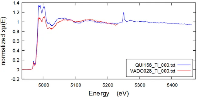
Fig. 23 Comparative titanium K-edge XAFS spectra of the QUI 156 and VADO 28. Note a prominent Ba LIII-edge peak at ~5240 eV………...28
Fig. 24 Comparative spectra of experimental titanium K-edge XANES spectra of QUI 156 (first), and calculated spectra of TiO2-rutile of different cluster radii: 6Å (second), 5.5Å (third) and 5Å
(the last)………..28 Fig. 25 Results of linear combination fitting in ATHENA of VADO 118 Ni K-edge XANES spectrum……….29 Fig.26 A comparative “survey scan” over electron-binding energies characteristic of core shell electronic energy levels of VADO 118, VADO 28 and QUI 156 filters before sputtering. The individual peaks are labelled by the element and core shell energy. Other peaks arising from secondary Auger electrons are labelled in standard KL format………,……..30 Fig.27a A detailed C1s XPS spectrum of QUI 156 resolved into signals assigned as reported in the discussion part………31
vi Fig.27b A detailed C1s XPS spectrum of VADO 118 resolved into signals assigned as reported in the discussion part……….……….……31 Fig. 27c A detailed C1s XPS spectrum of VADO 28 “new” resolved into signals assigned as reported in the discussion part……….……..32 Fig. 28 A detailed O1s XPS spectrum of VADO 28 “new” resolved into signals assigned as reported in the discussion part………33 Fig. 29 A detailed Si2p XPS spectrum of VADO 28 “new” resolved into signals assigned as reported in the discussion part………33 Fig.30a A detailed N1s XPS spectrum of VADO 28 “new” resolved into signals assigned as reported in the……….34 Fig. 30b A detailed N1s XPS spectrum of VADO 118 after 10 min of sputtering resolved into signals assigned as reported in the discussion part……….34 Fig.30c A detailed N1s XPS spectrum of QUI 156 resolved into signals assigned as reported in the discussion part………35 Fig. 31 A detailed Na1s XPS spectrum of VADO 118 after 10 min of sputtering resolved into signals assigned as reported in the discussion part………..36 Fig. 32a A detailed Fe2p XPS spectrum of VADO 28 “new” resolved into signals assigned as reported in the discussion part………37 Fig. 32b A detailed Fe2p XPS spectrum of VADO 118 after 30 min of sputtering resolved into signals assigned as reported in the discussion part……….37 Fig. 33a A detailed Ca2p XPS spectrum of VADO 118 after 30 min of sputtering resolved into signals assigned as reported in the discussion part………,………38 Fig. 33b A detailed Ca2p spectrum of VADO 28 “new” (bottom) resolved into signals assigned as reported in the discussion part………38 Fig. 34 An experimental sodium sulphate spectrum along with calculated in FDMNES sodium sulphate decahydrate spectrum using FDM and cluster radius of 6Å……..……….40 Fig. 35 An experimental sodium sulphate spectrum (the last) along with calculated spectrum using FDM and cluster radius of 6Å (the first), spectra od sodium sulphate decahydrate using cluster radii of 4.1Å (the second) and 6Å (the third) ………...41
vii Fig. 36 An experimental sodium sulphite spectrum along with calculated spectrum using FDM and cluster radius of 6Å ………..…….42 Fig. 37 Sulphur K-edge XANES spectra of sulphate and sulphite forms of sulphur. The progressive shift of the absorption-edge is shown [2] ……….….42 Fig. 38 An experimental sodium sulphite spectrum (the last) along with calculated spectra using FDM and cluster radius of 5Å (the first) and 6Å (the second) ……….…….43 Fig. 39 Database zinc sulphide spectrum along with calculated spectrum using FDM and cluster radius of 8.5Å……….……...43 Fig. 40 Database zinc sulphide spectrum (the last) along with calculated spectra using FDM and cluster radius of 6.5Å (the first), 8.5Å (the second) and 9.5Å (the third)……….………44 Fig. 41 Selected normalized pre-edge region (Fe K-edge) and the best fit obtained (Origin) of VADO 28, VADO 118 (top), QUI 156 and Fe2O3 (bottom)……….…….46
Fig. 42 (top) (C) The Fe K-edge pre-edge region of [Fe(H2O)6][SiF6] including the experimental
data, a fit to the data (- - -), the background function (--), and the individual pre-edge peaks from the fit (°°°). The inset displays the second derivative of the data and the second derivative of the fit (- - -). (D) Ligand field analysis of [Fe(H2O)6][SiF6] (E) Theoretical simulation of the pre-edge
region for [FeCl6] [7] (bottom) The pre-edge fit for FeSO4*7H2O done in Origin…………..……47
Fig. 43 (top) (C) Fit to the Fe K-edge pre-edge region of Fe(acac)3 including the experimental data
(s), a fit to the data (- - -), the background function (--), and the individual pre-edge peaks from the fit (°°°). The inset displays the second derivative of the data (- - -). (D) Systematic analysis of the octahedral pre-edge features. (E) Theoretical simulation of the pre-edge region for [FeCl6]3- [3]
(bottom) The pre-edge fit for Fe(NH4)(SO4)2*12H2O done in Origin………..………48
Fig. 44 Summary of the pre-edge characteristics for the binary mixtures between IVFe2+, VIFe2+,
IVFe3+ [4]………50
Fig. 45 Summary of pre-edge region fittings showing the centroid positions vs pre-edge intensity……….50 Fig. 46 A unit cell of hematite (left). Fe atoms are displayed in gold, O in red. A local fragment of the unit cell with local coordination (right). The picture displays both Fe-O and Fe-Fe interactions……….52
viii Fig. 47 Comparison of the experimental (-) and theoretical (…) kn-weighted EXAFS signals (upper
panels) and the corresponding Fourier Transform (FT) of the kn-weighted EXAFS for filter samples at the Fe K-edge. The different level of S/N reflect the relative abundance of the Fe in the filters. Because of the higher concentration, the EXAFS analysis of the VADO118 sample has
been computed in K2………55
Fig. 48 Selected normalized pre-edge region (Ti K-edge) and the best fit obtained (Origin) of QUI 156 (top) and VADO 28 (bottom)……….57
Fig. 49 Derivative plots of the K-edge spectra of vanadium……….58
Fig. 50 Vanadium XANES spectrum of the NIST urban PM SRM.[6]……….58
Fig. 51 O 1s evolution of components 1 (top) and 2 (bottom) in VADO 118……….61
Fig. 52 The evolution of N 1s components 1 and 2 with sputtering time of VADO 118 filter….…62 Fig. 53 The evolution of O, Si, C (left) and of Fe, N, Na (right) at.% with sputtering time in VADO 118……….63
ix
LIST
OF TABLES
Table 1 XPS measurement parameters……….………….…14 Table 2 Results of linear combination fitting in ATHENA of QUI 156, VADO 118 and VADO 28 Fe K-edge XANES spectra…………..………..……….45 Table 3 Pre-edge characteristics of reference iron compounds and filters and their comparison with literature values………..…49 Table 4 Structural parameters from EXAFS fitting results of filter samples. The estimated parameter errors are indicated in parentheses……….…54
x
ABSTRACT
Respirable fractions of airborne ambient particulate matter (PM), specifically PM10 and PM2.5,
have been identified over the years as potential health hazards. Moreover, there is a big concern about potentially toxic species that can dissolve in lung fluids and bloodstream. This toxic species can be either organic or inorganic in origin. Due to chemical complexity, extremely small particle sizes, small sample size collected on filters, analysis of such samples is quite problematic. The technique that has a great potential for elemental speciation of fine PM inside the bulk of the filter is a synchrotron-based X-ray Absorption Fine Structure Spectroscopy. This technique allows to identify the form of an occurrence of an element in the complex mixture, complementing compositional elemental data obtained by X-ray fluorescence and Proton-Induced X-ray Emission (PIXE). Additionally, XAFS is non-destructive and sensitive to parts-per-million (ppm) concentration levels of many elements when the signals are detected in fluorescence configuration. However, it is well known that chemical composition of airborne PM on the surface differs from that of the core. Moreover, many studies have shown that there is a good correlation between the surface composition of aerosol particles and their role in environmental processes, such as atmospheric scavenging and cloud condensation nuclei. Therefore, an X-ray Photoelectron Spectroscopy was employed to investigate the surface composition of PM. XPS is a non-destructive technique that requires minimum sample preparation. Furthermore, XANES K-edge spectra simulations using FDMNES code were performed in order to simulate lacking reference data for elements in scarce amounts. We went even further and performed FDMNES calculations for intermediate energy of sulphur K-edge. Previously such XAS simulations were done in solitary cases, therefore our interest was justified. Following the pre-edge and XANES analyses outcomes of the three investigated filters, and by considering the relative abundance of the metals in them, an EXAFS analysis at the Fe K-edge only was performed. It provided quantitative data of the selected metal core bonding, was performed. In particular the local atomic environment of the Fe site has been revealed, providing bond length referring mostly to the first coordination shell.
1
CHAPTER I INTRODUCTION
I-1 PMI-1-1 Air Pollution: historical aspects
In the 17th century, the coal burning near the palace at Westminster was forbidden by Queen Elizabeth I because of the offensive nature of smoke, and therefore the factories were moved away from London. Already in the 19th century, clinicians in England linked various lung diseases to air pollution. Nonetheless, a proper legislation to control air pollution was lacking in many industrial countries, until the major industrial air pollution episodes occurred in the Meuse Valley (Belgium, 1930), and in Donora Valley (Pennsylvania, United States, 1948) and in urban London (December 1952). In Belgium and US, air pollution was caused by excessive smoke from coal-burning domestic appliances and industrial furnaces, whereas in London, a dense fog occurred during inversion weather and lasted for four days. The detected concentrations of smoke particles and sulphur dioxide were 10 times of normal levels. Almost 4,000 deaths occurred during or after the episode, mostly of elderly people with chronic heart and lung diseases. Later, in the 1970s and 1980s many big cities had serious air pollution episodes such as Chicago, Mexico City, Lagos, Cairo, Tokyo etc. As a consequence, many developed countries introduced environmental legislation and created environmental protection agencies[8].
The introduction of new clean air regulations led to the reduction of pollution episodes in urban areas, elimination of winter smog (London-type pollution), and significantly improved levels of photochemical pollutants (California-type pollution) because of aggressive controls on vehicle exhausts and industrial fumes. But the problem of adverse health effects and excess deaths by airborne particulate matter (PM) in urban areas were not eliminated, as it was believed by an extensive review of Holland et al [9].
The reason that PM became very important air pollutants in recent decades and their adverse health effects became more hazardous is that air pollution in urban areas has changed. Air pollution from combustion of traditional fossil fuels (biomass, coal, wood, crude oil, diesel with high content in sulfur) is now in much lower concentrations than 30 to 40 years ago because of better and cleaner technologies, but other pollutants have gained prominence, such as fine and ultrafine PM, because of a dramatic increase in motor vehicle use worldwide with the consequent rise in exhaust emissions in urban areas. Nowadays, airborne PM is found not only in big cities but also in small and large towns, and their size distribution and composition is now more varied, e.g. they may contain heavy metals, PAHs, etc.[8].
2
I-1-2 Particulate matter composition and origins
Particulate matter (PM) is a complex, heterogeneous mixture that changes in time and space. It encompasses emissions from both natural and man-made sources. Natural sources include wind-blown dust, sea salt, volcanic ash, pollens, fungal spores, soil particles, the products of forest fires and the oxidation of biogenic reactive gases. Manmade sources include fossil fuel combustion (especially in vehicles and power plants), industrial processes (manufacturing metals, cement, lime and chemicals), construction work, quarrying and mining activities, cigarette smoking and wood stove burning. The main source of PM in urban areas is road transport in addition to the burning of fossil fuels in power stations and factories. Components of traffic-derived PM include engine emissions and wear, brake and tyre wear and dust from road surfaces. The largest single source of airborne PM from motor vehicles is derived from diesel exhaust (diesel fuel combustion results in many more particles than gasoline engines). Owing to the increase in the number of new cars with diesel engines in industrialised countries, diesel exhaust particles (DEPs) account for most airborne particulate matter (up to 90%) in the world’s largest cities. These particles are composed of a carbon core upon which high-molecular weight organic chemical components and heavy metals deposit. One of the most important distinctions of particulate pollution is based on how the particles are introduced into the atmosphere. [10].
The behaviour of particles in the atmosphere and within the human respiratory system is determined largely, but not wholly, by their physical properties which have a strong dependence on size, varying from a few nanometres to tens of micrometres. The class of coarse particles consists of particles having diameters greater than 2.5µm, the most widespread being PM2.5 and
PM10. This class includes the most visible or obvious forms of PM such as black smoke, soil, dust
from roads and building sites, large salt particles from sea spray, mechanically generated particles, as well as some secondary particles. Coarse particles also include pollen, mould, spores and other plant parts. PM10 denotes all ambient PM (i.e. ultra-fine, fine and coarse particles) having a
diameter of 10µm or less and are sometimes termed “thoracic” particles in that they can escape the initial defences of the nose and throat and penetrate beyond the larynx to deposit along the airways in the thorax[10].
I-1-3 Health hazards
Over the years exposures to ambient PM have been related to enhanced mortality and morbidity. PM exposures were reported to induce oxidative stress, pulmonary inflammation and modulate the immune responses of the lungs. Moreover, the PM were linked to various respiratory infections such as pneumonia, especially among the elderly. Previously, the toxicity of PM has been related to the particle size and not to its composition, however in last years it is being discovered that the
3 composition of PM strongly determines its toxicity[11, 12]. Associations between chemical composition and particle toxicity tend to be stronger for the fine and ultrafine PM size fractions[8]. Janssen et al. have demonstrated, that exposure to air pollution is associated with reductions in lung function and growth, asthma, allergic rhinitis and respiratory infections in children. The reason that children are more vulnerable than adults is in the higher permeability of their airways to air pollutants compared to adults and the immaturity of their respiratory defence mechanisms[10, 13].
4
I-2 X-ray Absorption Fine Structure Spectroscopy
X-ray Absorption Fine Structure spectroscopy is a unique tool for studying at the atomic structure at a molecular level, being highly sensitive to the local structure around selected elements that are contained within a material. The main advantage of this technique is that it can be applied not only to crystals, but also to materials without a long-range order: amorphous systems, glasses, disordered films, solutions, liquids, metallo-proteins, and in this work, particulate matter. Moreover, XAFS is also an electronic spectroscopy, that measures transitions between bound initial states and continuum final states[14].
I-2-1 Physics of XAFS
XAFS is intrinsically a quantum mechanical phenomenon that is based on the X-ray photoelectric effect, in which an incoming X-ray photon is absorbed by an atom, followed by freeing an electron from an inner atomic orbital (Figure 1). The “photoelectron” wave scatters from the atoms surrounding the absorbing atom, creating interferences between the outgoing and scattered parts of the photoelectron wavefunction, which provides information about the structure, structural disorder and thermal motions of neighbouring atoms. Other phenomena occurring are heat, X-ray fluorescence and production of electrons (the detection of which is at the basis of an X-ray photoelectron spectroscopy experiment), and of course the scattering of X-rays which is another fundamental X-ray-material interaction. This scattering could be either coherent, also called elastic (i.e., X-ray diffraction, where the scattered photons interfere with each other) or incoherent, leading to the family of inelastic scattering-based techniques[3].
5 As displayed at the bottom of Figure 1, the absorption of X-rays can be measured quantitatively, and it follows a similar exponential decay given by the Beer-Lambert law which describes optical transitions. The quantity of interest here is called linear absorption coefficient and it can be considered analogous to the absorbance in UV-vis spectroscopy. It is measured in [cm−1]. Actually, because of its applicability to all states of matter, it is more convenient to use the mass absorption coefficient μm obtained by normalization to the density of the material ρ, that is, (μ/ρ); therefore,
the dimension becomes [cm2/g]. The absorption coefficient describes how strongly X-rays are absorbed as a function of energy E. In general, matter becomes more transparent to X-rays at higher energies; that is, X-rays are more penetrating following a decreasing function proportional to (1/E3) of the absorption cross-section μ(E). However, at specific energies that are element-specific, there is a sudden increase in the cross section, also called X-ray absorption edge. This dramatic increase of the absorption is due to the photoelectric effect[3, 14]. In order to observe such an edge, the X-ray photon has to have a sufficient energy to liberate electrons from the low-energy bound states in the atoms. Absorption edges were first measured by Maurice de Broglie in 1913, and in 1920 Hugo Fricke first observed the “fine structure” – energy-dependent variations in μ(E). Afterwards, despite the enthusiasm about this new technique, the theoretical explanation of XAFS remained vague. Only in the 1970s Stern, Sayers and Lytle had clarified the essential points of a theory of XAFS and showed that XAFS could be a practical tool for structure determination.
The X-ray photoelectric process which gives rise to such an absorption is summarized in Figure 2.
An X-ray photon is absorbed by an atom, and the excess energy is transferred to an electron which is expelled from the atom, leaving it ionized. This electron is called photoelectron, and we will see how it is responsible for the EXAFS mechanism. The electron vacancy created in the photo absorption process leaves the atom in a very unstable condition and therefore two competing processes may occur. The first is X-ray fluorescence, in which a higher energy core-level electron fills the deeper core hole, emitting an X-ray of well-defined energy. This provides a unique signature of the atoms constituting the material once those photons are collected by a detector, as in X-ray fluorescence spectroscopy (XFS). The second process (for de-excitation of the core hole) is the Auger effect, in which an electron drops from a higher electron level and consequently, a second electron is emitted into the continuum. The measurement of these electrons is made possible by Auger spectrometers. In the hard X-ray region (>2 keV), X-ray fluorescence is more likely to occur than Auger emission, but for lower energy the Auger process dominates.
6
Figure 1 The photoelectric absorption process which creates a core hole, and its relaxation by fluorescent X-ray emission or Auger electron emission (taken from Giorgetti M.)[3]
I-2-2 XANES and EXAFS regions
X-ray Absorption Near Edge Structure (XANES) starts at absorption edge (Eo) and spans for
approximately 30 eV. In this region a core electron is excited into a bound empty valence state. The shape and intensity is characteristic of the oxidation state, number and type of atoms bonded to the excited atom. Intense peaks at the top of the edge are historically called “white lines”, because of their appearance on photographic plates[14]. The most common and the simplest interpretation of the XANES region is an identification of the oxidation state of an element. When the electron density around the absorbing atom decreases, its affinity towards electrons increases,
7 resulting in the shift of the absorption edge to slightly higher energies. These shifts of the order of few eV act as fingerprints of specific oxidation states. Generally, the edge energy is assigned as the position of first inflection point at the absorption edge, or the maximum at the derivative spectrum.
Additionally, by employing linear combination fitting techniques (LCF), the amounts of different components giving unique spectral features to XANES spectra, can be determined. This is made possible by the peculiar property of mass-absorption coefficients, which can be added together when multiple components are present. Also, XANES spectra can also be calculated. Among several programs performing such calculations, in this work the FDMNES code was employed. The FDMNES (Finite Difference Method Near Edge Structure) package is an ab initio code, which is based on building clusters around the absorbing atoms and performing several independent calculations when there are several non-equivalent absorbing atoms[15].
Another part of the XAS spectrum that comes after the XANES region and ranges to approximately 1000 eV above the edge is called Extended X-ray
Absorption Fine Structure spectrum (EXAFS). The EXAFS phenomenon arises from the quantum-mechanical interference resulting from the scattering of a photoelectron by the potential of the surrounding atoms.
This is seen from Figures 3 and 4 where the photoelectron emitted by the photoabsorbing atom (blue) propagates as a spherical wave and spreads out over the solid. At this point the mechanism can be different in case of an isolated atom (Figure 3) or a coordinated atom on (Figure 4). In the latter case, the emitted photoelectron is reflected off by the neighbouring atoms (yellow) to the absorbing atom and so does every atom in the material. The amplitude of all the reflected electron waves adds either constructively or destructively to the spectrum of the absorbing atom and hence the X-ray absorption coefficient exhibits the typical oscillations depicted at Figure 4 (bottom).
Figure 2 Emission of a photoelectron for an isolated atom (adapted from Giorgetti M.)[3]
8 A crucial issue is the recognition that the photoelectron is not infinitely long lived but decays as a function of time and distance, therefore, the EXAFS cannot probe long-range distances. EXAFS can give only local structural information, of about several angstroms around the selected atomic species. Of course, this mechanism does not happen in the case of isolated atoms like Ar gas, which leads to the corresponding X-ray absorption edge to appear featureless as observed in Figure 3 (bottom). From the time frame of the EXAFS phenomenon it is helpful to underline that this takes place at a time scale much shorter than that of atomic motion (also vibrations), so the measurement is a sum of instantaneous spectra of molecules at different stages of their vibrational cycle. This results in a damping of the EXAFS oscillations and is normally considered in the data analysis by means of an EXAFS Debye-Waller like factor. EXAFS should be considered as a bulk technique, because all the materials under investigation contribute to the overall shape of the XAS spectrum. As the oscillations in absorption are related to neighbouring atoms, the EXAFS region gives information about the number and type of neighbouring atoms and their distance to the absorbing atom [3, 16]. As a customary, in order to obtain the relevant structural parameters from an EXAFS features the experimental spectrum is fitted with a suitable structure. In this work, the fit obtained for an Fe K-edge case will be presented.
I-2-3 Synchrotron radiation
At the same time as XAFS spectroscopy was developing, research on synchrotron radiation was equally progressing. In the 1970s, when Stern, Sayers and Lytle were completing XAFS theory, the first synchrotron radiation facilities were developed. Nowadays, almost all XAFS experiments are performed at Synchrotron Radiation Sources (SRS) due to a high energy tuneable X-ray beams that are produced there. SRSs were the “bonuses” coming from high-energy physics experiments, which were later adapted to produce high-energy electromagnetic radiation with desirable spectral characteristics. Electrons moving close to the speed of light within an evacuated pipe are guided
Figure 3 Emission of a photoelectron for a coordinated atom. The absorption coefficient measured at a central atom threshold shows a fine structure due to the presence of neighboring atoms (adapted from Giorgetti M.)[3]
9 around a closed path of 100-1000 meters circumference by vertical magnetic fields. When the trajectory bends, the electrons accelerate (change velocity vector). Accelerating charged particles then emit electromagnetic radiation[14].
I-3 X-ray Photoelectron Spectroscopy
X-ray photoelectron spectroscopy was developed in the mid-1960s by Kai Siegbahn and his research group at the university of Uppsala, Sweden. The technique was first called ESCA (Electron Spectroscopy for Chemical Analysis). Later, in 1981, Siegbahn was awarded the Nobel Prize for Physics for his work with XPS.
The XPS experiment is based on irradiating a solid in vacuo with monoenergetic X-rays and by analysing the energy of the electrons emitted. The spectrum is a plot of the number of detected electrons per energy interval versus their kinetic energy. Each element has a unique spectrum with the mixture of elements giving the sum of the peaks of individual constituents. As the mean free path of electrons in solids is very small, the detected electrons originate from the top few atomic layers only, which makes XPS unique surface-sensitive technique. Quantitative data can be obtained from peak heights or peak areas, and identification of chemical states can be concluded from the exact measurement of peak positions and separations [17].
I-3-1 Principles of the technique
XPS proceeds by irradiating a sample with monoenergetic soft X-rays, generally Mg Kα (1235.6 eV) or Al Kα (1486.6 eV), and by analysing the energy of the detected electrons (Figure 6). These photons (penetrating power 1-10 μm) interact with atoms in the surface region, causing the electrons to be emitted by the photoelectric effect. The emitted electrons have measured kinetic energy given by:
KE=hν-BE-φs
where hν is the energy of the photon, BE is the binding energy of the atomic orbital from which the electron originates, and φs is the
spectrometer work function.
Figure 5 Relative binding energies and absorption cross-sections of uranium. The binding energy is proportional to the distance below the line indicating the Fermi level, and the ionization cross-section is proportional to the length of the line.[1]
10 BE is the energy difference between the initial and final states after the photoelectron has left the atom. As there is variety of possible final states of the ions from each type of atom, there is a corresponding variety of KE (Kinetic energies) of the emitted electrons. Furthermore, there is a different probability or cross-section for each final state. The Fermi level corresponds to zero BE (by definition), and the depth beneath the Fermi level in the Figure 5 indicates the relative energy of the ion remaining after electron emission, or the binding energy of the electron. The line lengths indicate the relative probabilities of the various ionization processes. The p, d and f levels become split upon ionization, leading to vacancies in the p1/2, p3/2, d3/2, d5/2, f5/2 and f7/2 levels. The
spin-orbit splitting ratio is 1:2 for p levels, 2:3 ford levels and 3:4 for f levels.
As each element has a unique set of binding energies, XPS can be used to identify and determine the concentration of the elements of the surface. Variations in the elemental binding energies (the chemical shifts) come from the differences in the chemical potential and polarizability of compounds. These chemical shifts are used to identify the chemical state of the materials being analysed.
Figure 6 Schematic of XPS experiment (taken from Crist V.)[18]
In addition to the photoelectrons emitted in the photoelectric process, Auger electrons may be emitted because of relaxation of the excited ions remaining after photoemission. This Auger
11 electron emission occurs roughly 10-14 seconds after the photoelectric event. The competing
emission of a fluorescent X-ray photon is a minor process in this energy range. In the Auger process (described previously on Figure 2 in XAFS introduction part), an outer electron falls into the inner orbital vacancy, and a second electron is simultaneously emitted with an excess energy. The Auger electron possesses kinetic energy equal to the difference between the energy of the initial ion and the doubly charged final ion, and is independent of the mode of the initial ionization. Therefore, photoionization leads to two emitted electrons - a photoelectron and an Auger electron. The probability of electron interaction with matter is way higher, so while the path length of the photons is of the order of micrometres, that of the electrons is of the order of tens of angstroms. Thus, while ionization occurs to a depth of a few micrometres, only those electrons that originate within tens of Angstroms below the solid surface can leave the surface without energy loss. These electrons which leave the surface without energy loss produce the peaks in the spectra and are the most useful. The electrons that undergo inelastic loss processes before emerging form the background[17].
MOTIVATION
OF
WORK
As described in the introduction, PM is a complex, heterogeneous mixture that changes in time and space. It encompasses many different chemical components and physical characteristics, many of which have been cited as potential contributors to its toxicity. Each component has multiple sources, and each source generates multiple components. Identifying and quantifying specific components and assigning chemical speciation represents one of the most challenging problems of analytical and environmental science. Generally, PM analysis is done using conventional techniques such as: gravimetry, inductively coupled plasma- mass spectrometry, atomic absorption spectroscopy etc. However, these techniques give information only about the elemental composition. In this work, we have successfully gone beyond the elemental characterization. By using core-level spectroscopy techniques we were able to obtain oxidation states, local structure arrangement and symmetry around selected sites and element quantification of different layers. Since the term speciation refers to the chemical form or compound in which an element occurs, this work can be considered an excellent example of chemical speciation.
12
CHAPTER
II
EXPERIMENTAL
AND
METHODS
II-1 PM sampling
Particulate matter deposited on filters were collected by the group of Prof. Laura Tositti (University of Bologna, Chemistry Department) from January till July 2012. For each collection, daily samplings of 24h duration were made. The two samples were named VADO and QUI, referring to their respective sampling zones. Therefore, several filters were available for analysis, which were identified by their sampling number. The VADO filter deposited PM10 on two different types of
filter (quartz and Teflon), while the QUI filter collected PM10 and PM2.5 on Teflon filters. In this
work only two VADO filters (VADO 118 and VADO 28) and one QUI 156 filter will be analysed.
The particulates were collected on two different types of filters: Teflon and quartz chosen according to the type of analysis planned, in order to obtain the most complete characterization of the particulates. Since, the PM is an extremely complex mixture where a number of organic and inorganic species are present, the choice of the filtering support was a critical aspect. The material constituting the membranes should be compatible with the type of analyte to be determined, and must not alter its composition through the chemical impurities. The degree of purity of the filters was verified every time a new set was acquired. Generally, the filters in quartz are used to determine and characterize the carbon fractions and the ions, while those in polymeric material are used to determine and characterize the inorganic fraction. The Teflon filters were used for PIXE analysis.
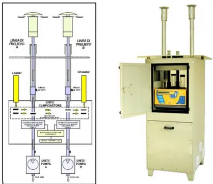
The sampling instruments have three units as shown on Figure 7:
1. Two sampling lines allowing the sampling of a particulate matter suspended in the atmosphere. Each line includes a sampling head with the function of collecting the exact size of PM, and with anti-wind and anti-rain properties.
Figure 7 The scheme and the photo of a sampler FAI SWAM Dual Channel
13 2. A filtering station with one or two filtering membranes on which PM is accumulated. 3. Two suction pumps, which intake air from the environment through the sampling heads,
the sampling tubes and the filtering membranes located in the filtering station.
At the end of every sampling cycle, the filters were transferred in a waste container. The operator could proceed to replace the filters (loading clean filters, unloading sampled filters) at any moment without interfering with the ongoing sampling. The two sampling pumps worked simultaneously and synchronously, to allow the collection of samples that are independent but perfectly equivalent in terms of the sampling’s time length. Furthermore, the sampler was equipped with a temperature controlling system, in order to limit the loss of semi-volatile species such as NH4NO3 and various
other organic species (adapted from Tositti et al.)
II-2 XAFS data collection
X-ray absorption near edge structure (XANES) and Extended X-Ray Absorption Fine Structure (EXAFS) spectra have been recorded at the XAFS of Elettra-Sincrotrone Trieste, Basovizza, Italy through the project №20150161 “Airborne particulate matter: metal speciation by X-Ray Absorption Spectroscopy” (project leader M. Giorgetti)[19] and further in-house experiments. The storage ring was operated at 2.0 GeV in top up mode with a typical current of 300 mA. Data have been recorded at the S, Ca, Ti, V, Cr, Mn, Fe, Ni, Cu, and Zn K-edges. The white beam was monochromatized using a fixed exit monochromator equipped with a pair of Si (111) crystals. Harmonics were rejected by using the cut-off of the reflectivity of the Platinum mirror placed at 3 mrad with respect to the beam upstream the monochromator and by detuning the second crystal of the monochromator.
Internal reference of Ca, Ti, V, Cr, Mn, Fe, Ni, Cu, and Zn foils were used for energy calibration in each scan. The first inflection point for Ca, Ti, V, Cr, Mn, Fe, Ni, Cu, Zn was set at 4038.5, 4966, 5465, 5989.9, 6539.0, 7112, 8333, 8979 and 9659 eV, respectively. This allowed a continuous monitoring of the energy during consecutive scans. No energy drifts of the monochromator were observed during the experiments. Spectra were collected with a constant k-step of 0.03 Å-1 with 3s/point acquisition time from 2200 to 3500 (S K-edge); from 3800 to 4800
eV (Ca K-edge); from 4700 to 5500 (Ti K-edge); 5200-6000 eV (V K-edge); 5700 to 6500 eV (Cr K-edge); from 6300 to 7100 (Mn K-edge); from 6900 to 7700eV (Fe K-edge); from 8100 to 8900 eV (Ni K-edge); 8700 to 9400 eV (Cu K-edge) and from 9400 to 10500 (Zn K-edge).
Spectra have been collected in fluorescence mode with the sample positioned at 45° with respect to the beam. The total fluorescence yield is measured as a function of the X-ray energy using a silicon drift KETEK detector. More than one spectrum was collected per each sample. The spectra were then averaged and normalized according to the standard procedure using the ATHENA program[20].
14
II-3 XPS data collection
Surface chemical characterization was performed using XPS in a Thermo Scientific Escalab 220i-XL spectrometer. Samples of ~0.25 cm2 of VADO 118 and ~0.09 cm2 of VADO 28 were supported on the sample holder with a carbon tape. For all XPS measurements the base pressure in the analyzer chamber was 1.0*10-8 mbar or less. The samples were excited by Al Kα (1486.68 eV) radiation from an Aluminium-Magnesium-twin-X-ray tube. Two lens modes were used: large area (LAE) and large area-XL (LAXL) depending on the size of the probe. When the latter mode was utilized the samples were irradiated with electron gun (flood gun) to prevent a positive charge accumulation. The layer composition and depth profiles of the VADO 118 and VADO 28 filters were investigated by sputtering with 1 keV Ar+ ions. The etching time was varied as 2, 10 and 30 min for VADO 118 filter and 10 min for VADO 28 filter.
The measurement parameters for the survey (white background) and detailed spectra (blue background) of the filters are summarized in Table 1 below. The measurement conditions were kept constant for all VADO 118 samples, and varied slightly for VADO 28 and QUI 156 as indicated in below.
Filter code Sputtering time (min) Energy range (eV) Pass energy (eV) Step size (eV) Dwell time (ms) Number of scans Lens mode QUI 156 0 -5 --1205 50 1 100 1 LAE VADO 118 0, 2, 10, 30 -5 -- 1205 50 0.5 100 1 LAE VADO 28 10 -5 -- 1205 50 0.5 100 1 LAXL QUI 156 0, 2, 10, 30 Depending on the element 10 0.1 300 5 LAE VADO 118 0, 2, 10, 30 20 0.1 300 4 LAE VADO 28 “old” 10 20 0.1 300 4 LAXL VADO 28 “new” 10 50 0.1 300 4 LAXL
Table 1 XPS measurement parameters
The data acquisition was performed using Thermo Scientific™ Avantage Software and data analysis with UNIFIT 2016 software[21, 22]. First the background was fitted using Shirley function followed by curve fitting using a convolution of Gaussian and Lorentzian functions.
15
II-4 FDMNES package details
The FDMNES (Finite Difference Method Near Edge Structure) package is an ab initio code, which is used to calculate the XANES (X-ray absorption near edge structures) spectra, which extend up to around 50 eV after the absorption edge. It builds clusters around the absorbing atoms performing several independent calculations when there are several non-equivalent absorbing atoms[15]. The challenging problem is to compute the final states, which depend on the local atomic structure, while the initial state is a core state easy to calculate. There are different ways to calculate these final states. One of them uses the local density approximation by considering clusters using the multiple scattering (MS) theory. Generally, MS theories use a muffin-tin approximation: averaging of the potential needed for the expansion of the wave functions. This approximation assumes the spherical shape of the potential in the atomic and outer sphere regions and volume averaged in the interatomic regions, which makes the results depend on the size of the interstitial region.
Another way to solve the Schrodinger equation using the local density approximation which avoids the muffin-tin approximation is the finite-difference method (FDM). The first formulation of FDM to solve the Schrodinger equation was given in the 1930s.
II-4-1 Finite difference method
In the FDM method a general way to solve differential equations by discretizing them over a grid of points in the whole volume where the calculation is made (Figure 8). In XANES, the equation is solved over a spherical volume, centred on the absorbing atom and the radii extending over a sufficiently large cluster. Inside this sphere the classical FDM equation is used. However, close to the ion core, the kinetic energy of the electron is very high, whereas in the region between two ion cores, it is much lower. A way to solve this discrepancy is in performing an expansion in
spherical waves in very little sphere around the atomic cores (0.5-0.7Å), assuming that potential is quite spherically symmetric in these areas. After writing the Schrodinger equation on all points of the grid, the potential must be introduced in the general matrix. As usual in standard XANES calculations, the local density approximation is used to calculate the potential. The FDM
Figure 8. General view of the region of calculation around the absorbing atom. Symmetry planes are used to reduce the area of calculation. This one is divided in three zones: (1) around the atomic cores, (2) between the atoms where the standard FDM calculation is used, (3) the outer sphere region. White points are at the boundary of the ion core. Gray points are at the boundary of the outer sphere (adapted from Joly et al.)[5]
16 formulation allows no approximation of the shape of the potential, thus avoiding the problem related to the classical muffin-tin approximation.
II-4-2 Muffin-tin calculations
The muffin-tin approximation corresponds to a monopolar representation of the potential and the potential in the interstitial region is constant. Overlapping muffin-tin spheres are used to take into account a part of the scattering power of the interstitial area. The use of overlapping spheres approximation is mathematically wrong, however when it is up to 10-15%, the advantages overcome the error. Sometimes, relatively good artificial agreement can even be reached when changing the interstitial potential and the muffin-tin radius. In order to have the best possible MS muffin-tin calculation, a muffin-tin radius and the interstitial potential value should be chosen carefully. The best radius is the one which minimizes the potential jump between the sphere and the interstitial area. For a muffin-tin approximation, generally a 10% to 15% overlap is used, because it has empirically been observed by the authors that with such overlap that the agreement with experiment is often the best [5].
II-4-3 The general procedure
All the sequences of the spectra calculations can be summarized in the following way: 1) From the molecule or the unit cell atom positions the code evaluates the non-equivalent and equivalent atoms with the symmetry operation relating them to each other. 2) For each non-equivalent and absorbing atom, a cluster is formed around it with a radius chosen by the user. The point group is evaluated, giving the shape of the scattering tensors and the useful representation to calculate. 3) For each cluster the final states are calculated. One of the two methods are chosen by the user: the finite differences method (FDM) or the multiple scattering theory (MST), the latter within the limits of the muffin-tin approximation (MT)[15]. The FDM is time consuming, so generally we start with MT approximation.
II-4-4 Details of the calculations
To interpret X-ray near-edge absorption spectra, we performed theoretical calculations in the framework of the MST within the MT potential approximation and the finite difference method with a full potential. Both methods were implemented in the FDMNES (2016) code (Joly, 2001). As mentioned earlier, the calculations started using MT approximation, but this method failed to reproduce spectral features, therefore only spectra calculated using FDM are presented here. Another thing to note is that the calculations were executed with a number of different sulphates, however only sodium sulphate was measured experimentally by us, therefore it is the only sulphate presented here.
17 For sodium sulphate spectra calculations clusters with radii of 6 Å and for sodium sulphate decahydrate clusters of 4.1 Å and 6 Å are presented here. The unit-cell parameter for Na2SO4*10H2O was taken from Ruben et al. with a space group P21/c [23]; for anhydrous Na2SO4
from Neues et al., Mincryst card №4721 [24]; for Na2SO3 crystal structure information was taken
from Zachariesen et al., with the space group C3i [25]and for sphalerite ZnS from Wyckoff et al.,
Mincryst card №4449[24]. The experimental sphalerite spectrum was taken from ESRF sulphur XANES database[26].
18
CHAPTER
III
RESULTS
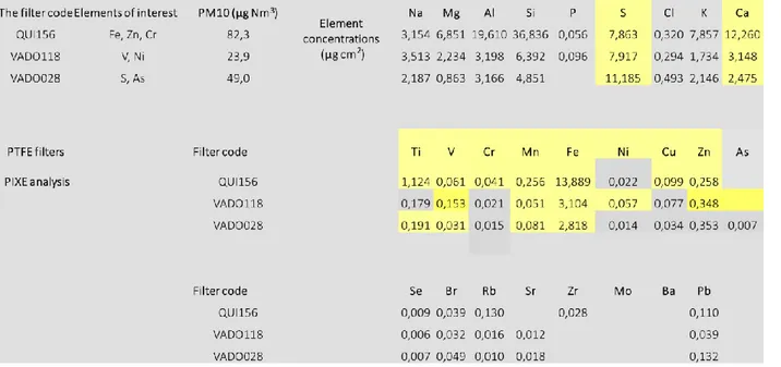
In order to perform a full characterization of the particulate matter deposited on filters, both bulk and surface analyses were carried out. This section is therefore organized as follows. The starting point were PIXE (Figure 9) and X-ray fluorescence response experiments, which allowed to list the elements present in the filters. The X-ray fluorescence response for QUI 156, VADO 118 and
VADO 28 is reported in the Appendix Figures A1, A2 and A3, respectively. As it is shown below on Figure 9, sulphur is a dominant inorganic non-metal element in the PM. Also, large quantities of Na, Mg, Al, Ca and Fe metals are present. These experiments set the feasibilities for each metal core K-edge experiments. Then, considering the concentrations of elements and peculiarities of synchrotron radiation experiment, a number of elements were analysed by XAS experiment (bulk) depending on their relative concentration. Later, K-edge reference spectra of reference compounds were recorded for these elements. In case of the absence of experimental reference data, XANES calculations using FDMNES code were performed. Finally, in order to analyse the surface of the filters, XPS experiments were carried out.
Figure 9 Element concentrations in QUI 156, VADO 118 and VADO 28 filters by PIXE analysis (data was kindly provided by the group of Prof. Tositti)
19
III-1 XANES
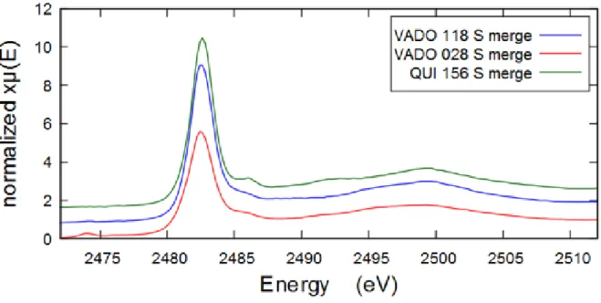
III-1-1 Results obtained with experimental reference XANES spectra III-1-1-1 Sulphur
Sulphur was present in all filters according to PIXE elemental analysis and fluorescence response data, and in VADO 28 filter there was more sulphur, 11.2 μg/cm2, than in VADO 118 and QUI 156 filter (roughly equal amounts of 7.9 μg/cm2 ). The comparative XANES S K-edge spectra of all filters are shown below on Figure 10. As we can see the VADO 28 has a weak peak at lower energies which is absent in other filters. QUI 156 filter shows more evident spectral features than the VADO filters.
The results of linear combination fitting for VADO 28 performed in ATHENA are demonstrated below on Figure 11 and fits for QUI 156 and VADO 118 filter can be found in the Appendix Figures A4 and A5.
20
Figure 11 Results of linear combination fitting in ATHENA of S K-edge spectrum of VADO 28 filter
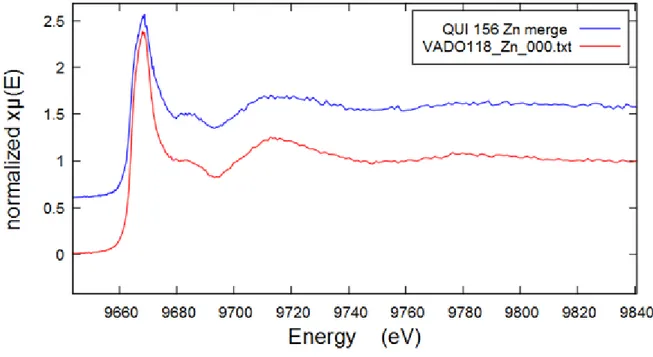
III-1-1-2 Zinc
Zinc was present in all filters according to PIXE elemental analysis and fluorescence response data, but Zn K-edge spectra were collected only for QUI 156 and VADO 118. The comparative XANES Zn K-edge spectra of all filters are shown below on Figure 12.
21 The results of linear combination fitting for QUI 156 performed in Athena are demonstrated above on Figure 13 and fits for VADO 118 filter can be found in the Appendix Figure A6.
III-1-1-3 Calcium
Calcium is present in abundance in all samples according to PIXE elemental analysis and fluorescence response data, therefore Ca K-edge spectra were collected for all filters. The comparative XANES Ca K-edge spectra of all filters are shown below on Figure 14.
Figure 13 Results of linear combination fitting in ATHENA of QUI 156 Zn K-edge XANES spectrum
22 Results of linear combination fitting for VADO 118 performed in Athena are demonstrated above on Figure 15 and fits for QUI 156 and VADO 28 filters are shown in the Appendix Figures A7-8. Figure 15 Results of linear combination fitting in ATHENA of VADO118 Ca K-edge XANES spectrum
23
III-2-1-4 Iron
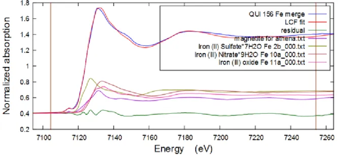
Iron was found in all filters according to fluorescence response data and PIXE elemental analysis, especially in abundance in QUI 156 filter, 13.89 μg/cm2. The comparative XANES Fe K-edge spectra of all filters are shown below on Figure 16. The results of linear combination fitting for QUI 156 performed in Athena is demonstrated below on Figure 17 and fits for VADO 118 and VADO 28 filters are shown in Appendix Figures A9 and A10.
Figure 16 Comparative iron K-edge XANES spectrum of the QUI 156, VADO 28 and VADO 118 filters
24
III-1-2 Results obtained with calculated reference XANES spectra III-1-2-1 Manganese
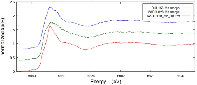
Manganese was present in all filters according to PIXE elemental analysis and fluorescence response data, but the amounts were rather low for VADO filters. QUI 156 filter had higher amount of Mn, 0.256 μg/cm2. The comparative XANES Mn K-edge spectra of all filters are shown below
on Figure 18.
Results of linear combination fitting for VADO 28 performed in Athena are demonstrated below on Figure 19. The fits for QUI 156 and VADO 118 filters are demonstrated Appendix Figures A11
and A12.
Figure 18 Comparative manganese K-edge XAFS spectra of the QUI 156, VADO28 and VADO 118 filters
25
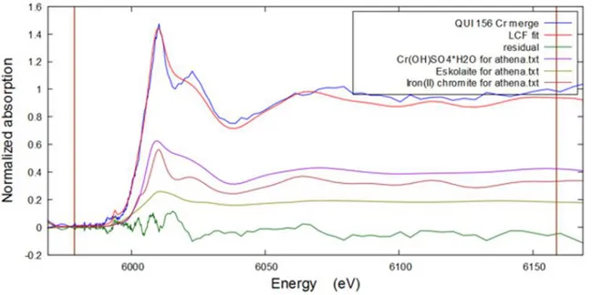
III-1-2-2 Chromium
Chromium was present in all filters, but in very small amounts. From fluorescence response data and PIXE elemental analysis, QUI 156 filter has the highest amount of 0.041 μg/cm2, therefore the Cr K-edge spectrum of QUI filter only was recorded. No reference data were collected for Cr samples, so the speciation was performed based on theoretical calculations only. The results of linear combination fitting for QUI 156 performed in Athena are demonstrated below on Figure 20.
26
III-1-2-3 Copper
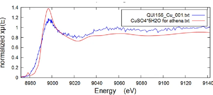
Copper content was very low, therefore XANES Cu K-edge spectrum of a rather low S/N ratio was obtained only for QUI 156 filter, which had the highest amount of Cu among other filters 0.099 μg/cm2 (based on PIXE analysis and fluorescence response data). No reference spectra were
recorded for Cu samples, so the assignment was performed based on FDMNES calculations only. The results of linear combination fitting for QUI 156 performed in Athena are demonstrated below on Figure 21.
27
III-1-2-4 Vanadium
The vanadium XAFS spectrum was collected for all filters, however, the vanadium content was rather low to give a good S/N spectrum (from PIXE analysis and fluorescence response data). The XAFS spectrum of the QUI 156, shown in Figure 22 below demonstrates a limitation of XAFS spectroscopy. The PM is a complex mixture of different elements, therefore the EXAFS region of one element might interfere with another element. In our case a strong LII-edge of barium limits
the EXAFS region for vanadium to about 120 eV, thus impeding the EXAFS analysis.. Nonetheless, the presence of barium does not affect the observation of the vanadium K-edge XANES region, and that information was still available for interpretation of the speciation of vanadium.
Figure 22 Comparative vanadium K-edge XAFS spectra of the QUI 156, VADO 118 and VADO 28 filters. Note a prominent Ba LII-edge peak at ~5620 eV.
28
III-1-2-5 Titanium
The titanium XAFS spectrum was collected for QUI 156 and VADO 28 filters, however, the titanium content was rather low in both filters to give a good S/N spectrum (from PIXE analysis and fluorescence response data). The comparative XAFS spectra of the QUI 156 and VADO 28 are shown on Figure 23 below. The spectrum of QUI 156 demonstrates a limitation of XAFS spectroscopy as in the case of vanadium. Here we see again barium limiting the EXAFS region of QUI 156. Strong LIII-edge of barium can be clearly seen on the spectra below. The results of
FDMNES calculations are plotted on Figure 24 below.
Figure 23 Comparative titanium K-edge XAFS spectra of the QUI 156 and VADO 28. Note a prominent Ba LIII-edge peak at ~5240 eV.
Figure 24 Comparative spectra of experimental titanium K-edge XANES spectra of QUI 156 (first), and calculated spectra of TiO2-rutile of different cluster radii: 5.5Å with FDM (second), 6Å with MT (third) and 5Å with MT methods (the last).
29
III-1-2-6 Nickel
According to PIXE elemental analysis nickel was present in all filters in very low quantities. XANES Ni K-edge spectrum was collected only for VADO 118 filter, which had the highest amount of Ni among other filters 0.057 μg/cm2 (from PIXE analysis and fluorescence response
data). No reference spectra were recorded for Ni samples, so an assignment was performed based on calculations only. However, it is important to note that a fair LCF fit might be due to imprecise spectra calculations and to a non-suitable broadening function. Nevertheless, the results of linear combination fitting for VADO 118 performed in ATHENA are demonstrated below on Figure 25.
30
III-2 XPS Results
III-2-1 Comparative survey scans
The multiple possible elements present in particulate matter can be identified in XPS survey scan because it spans a broad range of ejected core-shell electron energies. Figure 26 shows typical survey scans of PM collected on quartz (VADO118, VADO28) and PTFE (QUI 156) filters.
Figure 26 A comparative “survey scan” over electron-binding energies characteristic of core shell electronic energy levels of VADO 118, VADO 28 and QUI 156 filters before sputtering. The individual peaks are labeled by the element and core shell energy. Other peaks arising from secondary Auger electrons are labeled in standard KL format.
It can be noticed immediately that the comparative survey spectra (Figure 26) of two VADO filters are similar, revealing the presence of C 1s, O 1s, N 1s, Si 2p and Na 1s. Quartz – filter material, gives rise to Si 2p and O 1s signals. For QUI 156 filter the spectrum shows C 1s, O 1s, N 1s and F 1s peaks. The fluorine signal and double peak for carbon come from polytetrafluoroethylene (PTFE) - filter material. VADO 28 was collected using LAXL lens mode and a flood gun, however the survey spectrum does not reveal any significant differences.
31
III-2-2 Carbon
In order to identify the chemical state of the atomic species detected, the detailed spectra were collected. The acquisition energy range for C 1s spectra spanned from 270 eV to 305 eV. The detailed C1s spectra of QUI 156, VADO 118 and VADO 28 “new” with fitted backgrounds, are shown on Figures 27 a, b and c respectively. The VADO 118 C 1s spectra after 2, 10 and 30 min of sputtering can be found in Appendix Figures A13a-c.
Figure 27a A detailed C1s XPS spectrum of QUI 156 resolved into signals assigned as reported in the discussion part
32
Figure 27c A detailed C1s XPS spectrum of VADO 28 “new” resolved into signals assigned as reported in the discussion part
33
III-2-3 Oxygen
O 1s detailed spectra were acquired with energy range of 515-555 eV. Background-subtracted O 1s spectra of the VADO 28 “new” shown on Figure 28 below. The O1s spectra for VADO 118 at 0, 2, 10 and 30 min of sputtering and QUI 156 can be found in the Appendix Figures A14 a-e.
Figure 28 A detailed O1s XPS spectrum of VADO 28 “new” resolved into signals assigned as reported in the discussion part
III-2-4 Silicon
Si2p detailed spectra were acquired in the 90-120 eV energy range. Si2p spectra of the VADO 28 “new” with fitted background are shown on Figure 29 below.
34
III-2-5 Nitrogen
N1s detailed spectra were acquired in the energy range of 385-415 eV. Background-fitted N1s spectra of VADO 28 “new”, VADO 118 after 10 min of sputtering and QUI 156 are demonstrated on Figures 30 a, b and c, respectively. The N 1s spectra for VADO 118 at 0, 10 and 30 min of sputtering are shown in the Appendix A15a-c.
Figure 30a A detailed N1s XPS spectrum of VADO 28 “new” resolved into signals assigned as reported in the discussion part
Figure 30b A detailed N1s XPS spectrum of VADO 118 after 10 min of sputtering resolved into signals assigned as reported in the discussion part
35
36
III-2-6 Sodium
Na 1s was evident only in VADO 118 and VADO 28 survey spectra, and the detailed spectra were acquired in the energy range of 1055-1085 eV. Background-subtracted Na1s spectra of VADO 118 after 10 min of sputtering can be seen on Figure 31.
Figure 31 Na1s XPS spectrum of VADO 118 after 10 min of sputtering resolved into signals assigned as reported in the discussion part
37
III-2-7 Iron
Fe 2p became noticeable in VADO 118 survey spectrum only after 10 min of sputtering and the detailed spectrum was collected at the energy range of 690-745 eV. However, the spectrum after 10 min of sputtering is too noisy to obtain a good fit. Fe 2p spectra of VADO 28 “new” and VADO 118 after 30 min of sputtering also have low S/N ratio, nonetheless the fitting was attempted as shown on Figures 32 a and 32b.
Figure 32b A detailed Fe2p XPS spectrum of VADO 118 after 30 min of sputtering resolved into signals assigned as reported in the discussion part
Figure 32a A detailed Fe2p XPS spectrum of VADO 28 “new” resolved into signals assigned as reported in the discussion part
38
III-2-8 Calcium
Ca 2p became evident in VADO 118 survey spectrum only after 30 min of sputtering and the detailed spectrum was collected at the energy range of 335-370 eV. Ca 2p spectra of VADO 118 after 30 min of sputtering and VADO 28 “new” after 10 min of sputtering with fitted background are shown on Figure 33a and 33b.
Figure 33a A detailed Ca2p XPS spectrum of VADO 118 after 30 min of sputtering resolved into signals assigned as reported in the discussion part
Figure 33b A detailed Ca2p spectrum of VADO 28 “new” (bottom) resolved into signals assigned as reported in the discussion part
39
CHAPTER
IV
DISCUSSION
Metallic components of ambient air particulate matter are often cited as those most likely to exert health effects. They are generated by metallurgical processes, from impurities in fuel additives and in non-exhaust emissions (from mechanical abrasion such as brake- and tyre wear on vehicles). Interest is mainly targeted on transition metals such as Fe, V, Ni, Cr and Cu based on their potential to produce reactive oxygen species in biological tissues. A large fraction of ambient PM in many areas is derived from combustion processes and therefore, contains significant amounts of black carbon and organic carbon. Carbonaceous aerosol also originates from biological sources (e.g. viruses, pollen grains, plant debris) and contains secondary organic aerosol formed from the oxidation of biogenic and anthropogenic hydrocarbon emissions. More than 200 organic species have been identified, including alkanes, alkenes, aromatics, oxygenated compounds (including aldehydes, ketones and carboxylic acids), amino compounds, nitrates, polyaromatic hydrocarbons (PAH) and PAH derivatives[10]. Another widespread component is a wind-blown mineral dust tends to be made of mineral oxides. Sea salt is considered the second-largest contributor in the global aerosol budget, and consists mainly of NaCl originated from sea spray; other constituents of atmospheric sea salt reflect the composition of sea water, and thus include Mg, sulphate, Ca, K etc. In addition, sea spray aerosols may contain organic compounds, which influence their chemistry. Secondary particles originate from the oxidation of primary gases such as S and N oxides into sulphuric acid (liquid) and nitric acid (gaseous). The precursors for these aerosols— i.e. the gases from which they originate—may have an anthropogenic origin (from fossil fuel or coal combustion) and a natural biogenic origin. In the presence of ammonia, secondary aerosols often take the form of ammonium salts; i.e. (NH4)2SO4 and NH4NO3 (both can be dry or in aqueous
solution); in the absence of ammonia, secondary compounds take an acidic form as sulphuric acid (liquid aerosol droplets) and nitric acid (atmospheric gas), all of which may contribute to the health effects of particulates[15], [27]. In this section we show how many of the compounds listed above were identified by us as components of VADO and QUI filters.
The discussion part is presented according to an element under investigation. These elements are presented in the following order: S, Fe, Ca, Ti, V, Cr, Mn, Cu, Zn, Ni, C, O, N, Na and Si, because of the different joint experimental and theoretical approaches used for their analysis. In the discussion part we show how we have successfully gone beyond just elemental characterization. By using core-level spectroscopic techniques we were able to obtain oxidation states, local structure arrangement and symmetry around selected sites and element quantification of different layers.