A control oriented model for pressurizer transient dynamics

(1)

FACOLTÀ DI INGEGNERIA INDUSTRIALE E DELL’INFORMAZIONE

CORSO DI LAUREA MAGISTRALE IN INGEGNERIA NUCLEARE

A CONTROL-ORIENTED MODEL

FOR PRESSURIZER TRANSIENT DYNAMICS

Relatore: Prof. Antonio Cammi

Tesi di Laurea Magistrale di:

Alessandro Pini

Matr. 783319

(2)

FACOLTÀ DI INGEGNERIA INDUSTRIALE E DELL’INFORMAZIONE

CORSO DI LAUREA MAGISTRALE IN INGEGNERIA NUCLEARE

A CONTROL-ORIENTED MODEL

FOR PRESSURIZER TRANSIENT DYNAMICS

Relatore: Prof. Antonio Cammi

Tesi di Laurea Magistrale di:

Alessandro Pini

Matr. 783319

(3)

(4)

I

CHAPTER 3 – PRESSURIZER SIMULATION CODES 3.1 INTRODUCTION... 58 3.2 CAUSAL APPROACH ... 59 3.3 SIMULINK®_{MODEL ... 61} 3.4 ACAUSAL APPROACH ... 75 3.5 DYMOLA®_{MODEL ... 81} 3.6 RELAP5®_{... 85} 3.7 RELAP5®_{MODEL ... 89} 3.8 CONCLUDING REMARKS ... 91 3.9 REFERENCES ... 91

(5)

II

CHAPTER 4 – PRESSURIZER MODEL VALIDATION

4.1 INTRODUCTION... 92

4.2 VERIFICATION AND VALIDATION ... 94

4.3 FREE DYNAMICS SIMULATIONS RESULTS ... 97

4.4 SIMULINK®_{CONTROLLED-MODELS RESULTS ... 101}

4.5 DYMOLA®_{CONTROLLED-MODELS RESULTS ... 123}

4.6 RELAP5®_{CONTROLLED-MODELS RESULTS ... 131}

4.7 REFERENCES ... 140

CHAPTER 5 – THE LINEARIZED PRESSURIZER MODEL 5.1 INTRODUCTION... 142

5.2 THE LINEARIZATION PROCESS ... 143

5.3 TRANSFER FUNCTION, OPEN AND CLOSED LOOP ... 146

5.4 BEYNON-KURIDAN MODEL ... 149

5.5 LINEARIZATION AND STABILITY ANALYSIS ... 151

5.7 REFERENCES ... 159

CONCLUSIONS ... 160 REFERENCES... XV

(6)

III

LIST OF FIGURES

1.1 Pressurizer Scheme ... 7

1.2 Pressurizer Control Scheme ... 8

1.3 Shippingport Pressure Vessel ... 10

1.4 Functional Drawing of Shippingport Pressurizer ... 13

1.5 Pressurizer Transient Loss of Load from 51 MWe... 16

1.6 Pressurizer Transient Loss of Load from 74 MWe... 17

1.7 Pressurizer Transient Loss of Load from 105 MWe ... 18

2.1 Two-Regions-Single-Volume Pressurizer ... 28

2.2 Temperature Distribution Inside The Pressurizer ... 37

2.3 Two-Regions-Two-Volumes Pressurizer ... 39

2.4 Two-Regions-Three-Volumes Pressurizer ... 47

3.1 The Pressurizer Simulink®_{Model ... 61}

3.2 Input Block ... 62

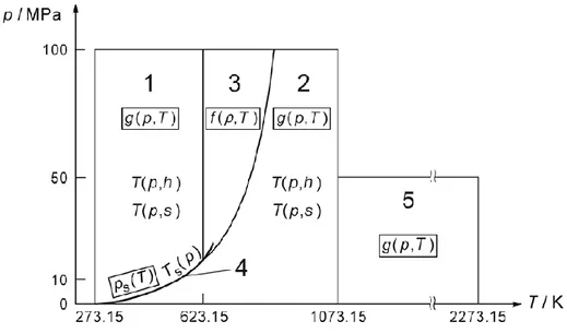
3.3 Regions And Equations Of Iapws-If97 ... 65

3.4 State Block Non-Equilibrium Model ... 69

3.5 State Block Equilibrium Model ... 70

3.6 Level Block Non-Equilibrium Model ... 71

3.7 Level Block Equilibrium Model ... 71

3.8 Wall Block Non-Equilibrium Model ... 72

3.9 Shippingport Control Block ... 73

3.10 Monitor Block ... 74

3.11 Conncetion Diagram Of The Acausal Simple Circuit Model ... 78

3.12 The simple circuit model using causal block-oriented modelling ... 79

3.13 Dymola®_{pressurizer components ... 82}

3.14 Dymola®_{pressurizer main componet ... 83}

3.15 Dymola®_{header component ... 84}

3.16 Dymola®_{pressurizer control... 84}

3.17 RELAP5®_{pressurizer model ... 90}

(7)

IV

4.2 Mass flow rate during 105 MW loss-of-load transient ... 96

4.3 Sprayers operations during 74 MW loss-of-load transient ... 97

4.4 Heaters operations during 105 MW loss-of-load transient ... 97

4.5 Pressure free-dynamics 74 MW loss-of-load for one-volume model ... 98

4.6 Pressure free-dynamics 74 MW loss-of-load for two-volumes model ... 98

4.7 Pressure free-dynamics 74 MW loss-of-load for three-volumes model ... 98

4.8 Sprayers operations during 105MW loss-of-load transient ... 99

4.9 Heaters operations during 105 MW loss-of-load transient ... 99

4.10 Pressure free-dynamics 105 MW loss-of-load for one-volume model...100

4.11Pressure free-dynamics 105 MW loss-of-load for two-volumes model ...100

4.12 Pressure free-dynamics 105 MW loss-of-load for three-volume model ...100

4.13 Pressure variation during 74 MW loss-of-load transient ...101

4.14 Pressure variation if Tsurge is the real one (284°C) ...102

4.15 Level variation during 74 MW loss-of-load transient ...102

4.16 Temperature variation during 74 MW loss-of-load transient ...102

4.17 Sprayers operations during 74 MW loss-of-load transient ...103

4.18 Heaters operations during 105 MW loss-of-load transient ...103

4.20 Pressure variation if Tsurge is the real one (284°C) ...104

4.21 Level variation during 105 MW loss-of-load transient...104

4.38 Temperature distribution during 74 MW loss-of-load transient ...111

4.39 Mass flow rates during 74 MW loss-of-load transient ...111

(8)

V

4.59 Sensitivity analysis for 1 volume model during 74 MW trans. ...120

4.60 Sensitivity analysis for 2 volumes model during 74 MW trans. ...120

4.86 Temperature distribution inside 1st_{volume during 74MW trans. ...133}

(9)

VI

4.88 Temperature distribution inside 3rd_{volume during 74MW trans. ...134}

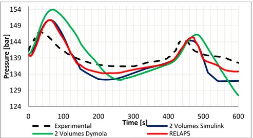
4.89 Pressure results comparison for 74 MW loss-of-load transient. ...134

4.90 Different mashes for Pressure 74 MW loss-of-load transient ...135

4.91 Different numerical methods for Pressure 74 MW transient. ...135

4.94 Temperature distribution inside 1st_{volume during 105 MW trans. ...137}

4.95 Temperature distribution inside 2nd_{volume during 105 MW trans...137}

4.96 Pressure results comparison for 105 MW loss-of-load transient ...138

4.97 Different mashes for Pressure 105 MW loss-of-load transient ...138

4.98 Different numerical methods for Pressure 105 MW transient ...138

5.1 Block diagram describing the system in the s-domain...147

5.2 Open-loop controlled system ...147

5.3 Closed-loop controlled system ...148

5.4 Negative-feedback controlled system ...148

5.5 Poles-zeros map with heat exchange ...155

5.6 Poles-zeros map without heat exchange ...156

5.7 The linearized pressurizer system ...157

5.8 1 kg/s insurge level response ...157

5.9 1 kg/s insurge pressure response ...157

5.10 1 kg/s outsurge level response ...158

(10)

VII

LIST OF TABLES

1.1 Shippingport History ... 9

1.2 Pressure Control Parameters ... 13

1.3 Instrumentation for loss of load transient test ... 14

2.1 Pressurizer regions description ... 29

2.2 Pressurizer state variables ... 33

2.3 Thermodynamic partial derivatives... 33

2.4 Pressurizer state variables ... 42

3.1 Numerical values of the coefficients and exponents of the dimensionless Gibbs free energy for region 1 ... 65

3.2 Numerical values of the coefficients and exponents of the ideal-gas part γ0_{of the} dimensionless Gibbs free energy for region 2 ... 67

3.3 Numerical values of the coefficients and exponents of the real-gas part γr_{of the} dimensionless Gibbs free energy for region 2 ... 68

(11)

VIII

ABSTRACT

This study develops a control-oriented model for the pressurizer subsystem of Pressurized Water Reactors (PWRs).

The purpose of this modelling activity is to faithfully reproduce the dynamic behaviour of the pressurizer along its entire range of operations using both block-diagrams and

object-oriented approach. For this reason Simulink®_{and Dymola}®_{pressurizer simulation}

programs are realized.

Regarding accuracy, the created model leaves behind previous control-oriented approaches: old control-oriented models used to provide rough reproductions of real physic transients occurring inside the pressurizer tank, while the new one is able to closely follow them. The studied model is based on the non-equilibrium multi-region approach: water and steam present in the pressurizer tank are treated as different phases and can be at saturation conditions or, respectively, at subcooled or superheated ones. No a priori assumptions are made concerning the particular thermodynamics process followed during transients. The basic mathematical model is derived from mass and energy conservation equations and includes all the important thermal-hydraulic processes which can occur inside the pressurizer. These processes are: spray condensation, bulk and surface condensation and evaporation, condensate fall and heat transfer from heaters. Furthermore, the model takes into account heat exchange processes between vapour and liquid regions and thermal dissipations between the entire pressurizer and the external ambient. To obtain the best achievable performances, the model is declined into three variants: complete lumped parameter and quasi 1D representations.

Each different version has been developed as a natural evolution of the previous one, therefore, in the following pages, zero-dimensional, two-volumes and three-volumes pressurizer models are presented in order of increasing complexity and accuracy.

Finally, the three models are compared with experimental data coming from Shippingport

(12)

IX

ESTRATTO

Questa tesi nasce con lo scopo di realizzare un modello, orientato al controllo, per la simulazione del comportamento dinamico di un componente fondamentale per i reattori nucleari ad acqua in pressione (Pressurized Water Reactor PWR): il pressurizzatore. Tale sistema, che ha il compito di mantenere la pressione dell’impianto entro un certo intervallo di valori, è tipicamente costituito da un recipiente in acciaio al carbonio rivestito internamente in acciaio inossidabile contenente in parte acqua e in parte vapore. Di forma generalmente cilindrica ad orientazione verticale, esso è collegato alla gamba calda del circuito primario e contiene riscaldatori elettrici nella parte inferiore ed un ugello per lo spruzzo di acqua, proveniente dalla gamba fredda, nella parte superiore. Quando la pressione nell’impianto tende a diminuire, parte dell’acqua contenuta nel pressurizzatore evapora: i riscaldatori sono quindi accesi per ristabilire la pressione nominale. Quando, per contro, la pressione tende ad aumentare, il vapore è condensato mediante l’azionamento di un sistema di spruzzatori.

La modellazione dinamica è di primaria importanza in un reattore nucleare e, nel caso specifico di un PWR, è essenziale simulare e prevedere l’andamento della pressione durante differenti transitori, al fine di operare il reattore in sicurezza o decidere le azioni di controllo e mitigazione necessarie in caso di eventuali incidenti.

Per questa ragione appositi programmi di simulazione del comportamento del pressurizzatore sono stati sviluppati già a partire dagli anni Cinquanta del secolo scorso. I primi modelli sono stati basati su un approccio a parametri concentrati in cui l’acqua e il vapore contenuti nel pressurizzatore sono trattati come una miscela omogenea in condizione di saturazione.

Successivamente sono stati studiati i cosiddetti modelli di non-equilibrio in cui acqua e vapore, considerati come due fasi separate, possono dare luogo, all’interno del volume del pressurizzatore, ad una qualsiasi combinazione degli stati termodinamici possibili. Vale a dire saturazione o sottoraffreddamento per la fase liquida, saturazione o surriscaldamento per quella gassosa.

In questo modo, considerando una semplice suddivisione in due regioni del pressurizzatore, si possono verificare quattro differenti stati: liquido saturo e vapore

(13)

X

saturo, liquido sottoraffreddato e vapore surriscaldato, liquido saturo e vapore surriscaldato, liquido sottoraffreddato e vapore saturo. Stati di surriscaldamento per la fase liquida non sono invece ammessi, in quanto in tali condizioni avviene un fenomeno di evaporazione di massa (bulk evaporation); analogamente la regione gassosa non sperimenta stati di sottoraffreddamento per il verificarsi di un processo di condensazione di massa (bulk condensation).

Con l’avvento dei cosiddetti codici di sistema (come ad esempio RELAP5®_{), attraverso i}

quali le autorità competenti impongono che l’impianto nucleare da licenziare debba essere simulato al fine di certificarne la sicurezza, può sorgere il dubbio che programmi di simulazione realizzati ad hoc per i singoli componenti di un reattore non abbiano più ragione di esistere.

Tuttavia questa perplessità, che inizialmente può sembrare ragionevole, entra rapidamente in crisi se si osserva che negli ultimi decenni si è assistito ad un sempre più massiccio uso di strumenti di simulazione molto diversi dai già citati codici di sistema.

Questi ultimi, infatti, benché siano certificati, affidabili e certamente fungano da standard di riferimento, sono affetti da un grande problema: possono richiedere ore per ricreare un singolo transitorio.

Questo punto debole, in particolare, non deve essere valutato solo dal punto di vista del tempo macchina, che in molti casi è una risorsa scarsa, ma anche tenendo presente che, durante la progettazione di un componente o di un impianto, devono essere accuratamente studiati anche il sistema e la logica di controllo.

In questo senso i codici di sistema, se da un lato permettono di ottenere simulazioni straordinariamente aderenti alla realtà, dall’altro impediscono un profonda integrabilità fra il modello dinamico del sistema stesso e il modello del sistema di controllo.

È quindi tangibile la necessità di sviluppare opportuni strumenti per la simulazione del comportamento di un impianto, gestito da un controllore dinamico, su intervalli temporali che possano comprendere pochi minuti, così come alcune ore. Per questo scopo si deve ricorrere a modelli non lineari, basati sui principi primi, che non si limitino a descrivere il comportamento del sistema attorno a un punto di equilibrio, ma permettano di abbracciare l’intero campo dei punti di funzionamento valutando anche condizioni di lavoro al di fuori di quelle progettuali.

Ritornando al caso del pressurizzatore, mentre i modelli di pura simulazione, da anni ormai sono orientati al già citato approccio di non-equilibrio termodinamico, quelli specificamente orientati al controllo continuano a fondarsi sull’ipotesi, molto lontana dalla realtà, che l’acqua e il vapore presenti nel suddetto componente possano essere trattati come una miscela omogenea in condizioni di saturazione.

In questo modo, i modelli appositamente sviluppati per lo studio del sistema di controllo, da un lato, essendo caratterizzati da una formulazione particolarmente semplice, permettono di studiare facilmente le caratteristiche dinamiche e la stabilità del sistema, dall’altro, invece, hanno scarse capacità nel riprodurre in modo effettivo i transitori reali. Di conseguenza si vuole creare un nuovo modello, che pur rimanendo “control-oriented”, sia fedele alla fisica dei processi che avvengono all’interno del pressurizzatore. Attraverso tale modello e alla sua aderenza alla realtà sarà possibile studiare l’influenza sulla dinamica del sistema di tutti i fenomeni che realmente entrano in gioco e sviluppare,

(14)

XI

di conseguenza, logiche di controllo più avanzate rispetto a quelle tradizionalmente applicate.

Alla creazione di questo nuova tipologia di simulazione è volto il seguente lavoro di tesi, il quale infatti si conclude con la realizzazione di un modello che non solo abbandona l’ipotesi semplificativa di sistema all’equilibrio termodinamico, ma supera anche l’approccio a parametri concentrati.

È importante sottolineare come lo studio compiuto sia il frutto di una progressiva evoluzione che ha come punto di inizio un approccio in parte “lumped parameter” in cui il pressurizzatore è diviso in due regioni a volumi variabili, una per la fase liquida ed una per il vapore, con il vincolo che il volume totale, ossia quello del recipiente, rimanga costante. A tali volumetti sono quindi applicati i bilanci di massa ed energia che comprendono anche fenomeni di scambio termico e processi di dissipazione del calore tra pressurizzatore e ambiente esterno.

Le equazioni di conservazione della massa, dell’energia ed il vincolo sul volume, i quali costituiscono un sistema fortemente non lineare, sono la base fondamentale dell’intero lavoro di tesi.

Bisogna sottolineare che la presenza del vincolo algebrico sul volume rende il sistema di equazioni sopra descritto non un classico sistema di equazioni differenziali ordinarie (Ordinary Differential Equation ODE), bensì un sistema di equazioni algebrico-differenziali (Differential Algebraic Equation DAE), che presenta alcune peculiarità e che per poter essere risolto, generalmente, deve essere ricondotto in forma di ODE. Per potere effettuare ciò, seguendo un approccio consueto, il vincolo sul volume deve essere derivato rispetto al tempo. In questo modo si ricava un’equazione differenziale governante la pressione del sistema. Ovviamente il sistema ODE ottenuto è anch’esso non lineare, inoltre, alcune grandezze che vi compaiono, cambiano a seconda dello stato termodinamico delle regioni cui fanno riferimento.

Sulla carta questo modello potrebbe bastare, tuttavia, grazie al confronto coi dati sperimentali (sono stati utilizzati quelli ricavati alla fine degli anni Sessanta del XIX secolo in seguito agli esperimenti condotti sul pressurizzatore della centrale di Shippingport) ci si può rendere conto che i risultati delle simulazioni sono in verità ben lontani dalla realtà. Questo fatto induce a supporre che la regione liquida non possa essere considerata puntiforme, ma sia necessario tener conto di una certa distribuzione di temperatura al suo interno.

A questo primo modello ne segue pertanto un secondo caratterizzato dal fatto che la ragione liquida è ora suddivisa, in altezza, in due volumi, di cui quello superiore rimane variabile e segue il vincolo sul volume totale del pressurizzatore, mentre quello inferiore è fisso. Confrontando nuovamente i risultati delle simulazioni con i dati sperimentali, si nota un notevole miglioramento delle prestazioni del modello.

Tuttavia, per ottenere risultati veramente soddisfacenti, un terzo modello conclude la serie. Quest’ultima evoluzione si basa sulla suddivisione della regione liquida in tre volumi, due costanti ed un terzo variabile.

È necessario infine sottolineare che solo i volumi variabili possono sperimentare diversi stati termodinamici, mentre quelli fissi, ovvero quelli che occupano le zone inferiori della regione liquida, permangono sempre nello stato di sottoraffreddamento. A priori ciò non

(15)

XII

si potrebbe imporre, ma l’analisi del pressurizzatore condotta usando RELAP5®_{lo mette}

evidenza. Infatti, con l’impiego di RELAP5®_{, è possibile ottenere risultati attendibili circa}

la distribuzione di temperatura presente nella regione liquida del sistema (per la quale mancano dati sperimentali) con cui validare il modello “control-oriented”.

Dalle elaborazioni effettuate da RELAP5®_{si evince che le regioni inferiori del}

pressurizzatore, durante i transitori di ingresso e uscita dell’acqua dal sistema, permangono sempre in condizioni di sottoraffreddamento. Questo fatto permette di semplificare, senza alcuna perdita di accuratezza, il modello. Se infatti anche tali regioni fossero soggette a cambiamento di stato termodinamico, le equazioni caratteristiche di tutto il sistema sarebbero ancora più complesse.

Questa procedura dimostra come i codici di sistema e codici ad hoc per il controllo non si escludano reciprocamente, ma possano essere usati sinergicamente per ottenere migliori risultati nel modo più semplice.

A questo punto sorge spontanea la domanda circa le modalità con cui i modelli descritti siano stati effettivamente implementati a calcolatore al fine di ottenere i risultati da confrontare coi dati sperimentali.

In particolare, sono stati seguiti due approcci differenti: tutti e tre i modelli sono stati

compilati utilizzando sia il linguaggio MATLAB-Simulink®, sia quello

Modelica-Dymola®. Questo al fine di creare dei programmi di simulazione che diano circa i

medesimi risultati, permettendo tuttavia di implementare i modelli matematici che ne stanno alla base in modalità completamente differenti.

Tradizionalmente i modelli “control-oriented” sono convertiti in codice usando il

cosiddetto approccio causale, su cui si basa Simulink®_.

In questo modo si realizzano modelli ingresso-uscita in cui il problema è formulato sfruttando i nessi di causalità presenti nel sistema.

Le equazioni che esprimono le grandezze di interesse (variabili di uscita) sono espresse in funzione di quantità note (variabili di ingresso), attraverso una serie rigidamente definita di operazioni impiegate per risolvere il problema considerato.

La forma che assume il modello risulta così più simile all’algoritmo usato per risolvere il problema, piuttosto che alla struttura fisica del sistema stesso, rendendo difficoltoso qualsiasi tentativo di recupero o approfondimento del lavoro svolto.

Le variabili di ingresso rappresentano le azioni compiute sull’oggetto in esame da agenti esterni che ne influenzano il comportamento, mentre le variabili di uscita rappresentano quanto del comportamento del sistema è di interesse: tra queste variabili vi è un rapporto di causa ed effetto, dato che l’evoluzione delle seconde descrive il modo in cui il sistema risponde alle sollecitazioni impresse dalle prime. In generale, però, la conoscenza del valore in un certo istante delle variabili di ingresso non è sufficiente ad individuare il valore, nello stesso istante, delle variabili di uscita: è allora necessario introdurre un terzo tipo di variabili, le variabili di stato, che descrivono la situazione interna del sistema. La formulazione causale del problema sfrutta una rappresentazione grafica basata sui cosiddetti schemi a blocchi che consente di mettere in luce con chiarezza le interazioni tra i diversi sottosistemi.

I diagrammi a blocchi costituiscono la formulazione naturale con cui descrivere un sistema di controllo, il quale è intrinsecamente procedurale. È per questa ragione che

(16)

XIII

l’approccio causale è il più diffuso per descrivere modelli orientati al controllo, in quanto permette di focalizzare immediatamente le grandezze sulle quali è possibile esercitare un’azione per gestire l’evoluzione del sistema.

Infine la necessità di dover pesantemente manipolare le equazioni per codificarle ed implementarle nell’ambiente di simulazione, porta ad una maggiore comprensione della dinamica e dei processi caratteristici del sistema.

Tuttavia l’aver imposto a priori, prima ancora di realizzare il modello, quali grandezze siano da considerare note e quali incognite, non permette di operare modifiche: se il modello dovesse essere adottato in nuovi contesti, molto probabilmente tali assunzioni potrebbero risultare violate e il modello di conseguenza essere inutile.

Negli ultimi anni, grazie all'aumento delle capacità di calcolo, si è però diffusa un’altra tipologia di modellazione basata sul cosiddetto approccio a-causale.

Si tratta di un modo strutturato di realizzare modelli direttamente basato sulle equazioni costitutive e sulle leggi di conservazione del sistema in esame, le quali determinano l’insieme di equazioni che deve essere risolto.

Realizzare modelli dinamici secondo questa formulazione del problema non richiede di specificare a priori quali grandezze debbano agire come ingressi e quali come uscite: le equazioni sono scritte in forma dichiarativa indipendentemente dalle condizioni al contorno e i nessi di causalità non sono specificati fino a quando le equazioni non sono risolte, in base alle condizioni al contorno imposte dal contesto applicativo. Per questo motivo, quando si parla di modellazione a-causale, spesso è anche usato il termine “modellazione fisica”, in quanto questo tipo di approccio è adatto per rappresentare la struttura fisica del sistema descritto. Il vantaggio principale della modellazione a-causale è che la direzione secondo la quale le equazioni sono risolte si può facilmente adattare di volta in volta in base al flusso di dati caratteristico della situazione cui si fa riferimento. In questo modo, l’attenzione rimane focalizzata sui componenti fisici del sistema, il cui comportamento è descritto da sistemi DAE. Per realizzare dei modelli a-causali è necessario selezionare i componenti e collegarli in uno schema: i modelli di ciascun componente sono formulati indipendentemente dalla conoscenza dei legami o delle equazioni che regolano altre parti del sistema. Partendo dal modello generale, che inquadra solo gli elementi fondamentali, è possibile arricchirlo (aggiungendo sensori, attuatori, ecc.) fino a renderlo completo. Con questo approccio, si riducono notevolmente le tempistiche e le difficoltà di modellazione, producendo modelli più comprensibili e vicini al mondo fisico. Per contro, è necessario che il simulatore sia in grado di effettuare un’analisi simbolica su sistemi DAE di grandi dimensioni.

Tra i vari interpreti, uno dei più affidabili e robusti è Dymola®_.

Per quanto detto, i programmi del pressurizzatore realizzati in Simulink®_{risultano essere}

più rigidi da un punto di vista di una futura implementazione come singolo componente in un sistema di modellazione più generale, come ad esempio quello di un intero reattore nucleare, mentre risultano certamente più comodi per lo studio e lo sviluppo di un sistema

di controllo. Al contrario i programmi realizzati in Dymola®_{sono di più semplice}

ri-utilizzo e di più facile interpretazione; lo studio del controllo è, invece, meno immediato. I risultati delle simulazioni del pressurizzatore, considerato come singola entità, sono comunque molto simili ad indicare che entrambi gli approcci sono validi e performanti.

(17)

XIV

La scelta dell’uno piuttosto che dell’altro dipende soltanto dal contesto di utilizzo del programma di simulazione.

Per valutare le caratteristiche di stabilità del sistema, si è infine proceduto alla linearizzazione attorno ad un punto di equilibrio del modello non lineare. Da questo studio si è giunti ad una conclusione particolarmente significativa: i processi di scambio termico, che nei modelli di pressurizzatore presenti in letteratura, sono spesso trascurati, divengono fondamentali per le proprietà di controllo dinamico del sistema. Solo se essi sono presi in considerazione, il pressurizzatore è un vero e proprio sistema dinamico, che può presentare tanto una risposta forzata dipendente dagli ingressi esterni, quanto una risposta libera funzione dello stato del sistema.

(18)

(19)

1

INTRODUCTION

The continuously increasing demand related to the development of safer and more effective nuclear power plants needs either the improvement or complete re-design of different components.

In this regard, dynamic simulation is an essential tool since the development of detailed dynamic models aids the study of a system in order to build or improve it. Modelling leads to deeper understanding of the behaviour of a system, to the optimization of its

technical specifications and to the discovery of its possible weaknesses.

Moreover, a model can be used to answer questions about a system without doing

experiments on the real object, especially when these might be too expensive, too

dangerous or the system needed for the experiment might not exist yet.

Of course experiments cannot be completely avoided. A model must be always validate with experimental data coming from facilities and prototypes. A model is seldom universal, it gives correct results only inside its range of validity depending on the assumptions on which the model itself is fulfilled.

There are different kinds of models depending on how the model is represented:

 Physical model: this is a physical object that mimics some properties of a real

system, to help answer questions about that system.

 Mathematical model: a description of a system where the relationships between

variables of the system are expressed in mathematical form. Variables can be measurable. Most laws of nature are mathematical models in this sense.

The kind of model developed in this study is the mathematical one. It will be represented in various ways, as equations and computer programs. In this regards, artefacts represented by mathematical models in a computer are often called virtual prototypes and the process of constructing and investigating such models is virtual prototyping.

Sometimes the term physical modelling is used also for the process of building mathematical models of physical systems in the computer if the structuring and synthesis process is the same as when building real physical models.

(20)

2

Within virtual prototyping there are two different ways:

 the causal approach

 the a-causal approach

Using tools, as MATLAB-Simulink®_{it is possible to realize ad hoc models of a system,}

based on the widespread causal approach: this modelling language makes use of block diagram to described the system. It is a refined representation of the behaviour of dynamical systems allowing a natural formulation of control problem. In fact they focalize directly on quantities on which it is possible to exercise an action to operate the evolution of the system.

In the causal approach, variables of the environment that influence the behaviour of the system (inputs) and variables that are determined by the system and may influence the surrounding environment (outputs) are a priori fixed and depend strictly on the boundary conditions. In these models, relationships between quantities are expressed using

assignments. An assignment statement sets and/or re-sets the value stored in the storage location(s) denoted by a variable name; in other words, it copies the value into the variable. In most imperative programming languages, the assignment statement (or expression) is a fundamental construct.

A very simple example of assignment is:

A=B I.1

Then the value of B is assigned to A.

However in a lot of systems the same variables act as both inputs and outputs. Precisely, you talk about a-causal behaviour if the relationships or influences between variables do not have a causal direction, which is the case for relationships described by equations. The equivalent equation formulation of the previous assignment example is:

f(A,B)=0 I.2

Which must be solved numerically.

Regarding the a-causal approach, one of the most promising programming languages is

Modelica®_.

Generally speaking, a system can be almost everything: in nuclear engineering it can be an entire power plant or one of its components whose properties must be studied.

Dynamic modelling has primary importance for a nuclear reactor, which can be licensed if and only if its safety systems and its capability to effectively respond to abnormal transient are verified by a special nuclear regulatory commission. For this purpose

certified programs, as RELAP5®_{, exist but they can take a long time to reproduce just a}

single transient, with the result that dynamic model of the system and control model can be coupled poorly.

(21)

3

Therefore the development of appropriate tools for the simulation of a nuclear power plant and its subsystems operated with dynamic control for any time interval is very attractive.

Historically models can be distinguished into two main families:

 Linear models, which have the advantage of being able to use simple and

systematic linear control design techniques, but also the disadvantage of being valid only when the system operates in a sufficiently small range around an equilibrium point. In fact, as almost every physical system contains nonlinearities, linear models usually derive from the linearization procedure, which is an approximation one, of the non-linear equation of the physical system.

 Non-linear model, which are based directly on fundamental principles without

linearization process, can describe the system not only around an equilibrium point, but also along the whole operating range. However they cannot use directly helpful tools which are available for their linear counterparts.

As far as a pressurized water reactor (PWR) is concerned, a very interesting subsystem to study is the so-called pressurizer.

As matter of fact, an accurate modelling of the pressurizer is needed to determine the pressure response of the primary coolant system, and thus to successfully simulate overall PWR nuclear power plant behaviour during normal operations and transients.

So the following study arises with the object to develop a simple but accurate model for the pressurizer component of PWR .

To be able to simulate all possible transients which can occur in a nuclear reactor, the model will be a non-linear one, but it will be subsequently subjected to the linearization procedure in order to do a preliminary study of the stability properties of the pressurizer system. The model will be based on a rigorous application of the first law of the thermodynamics:

I.3

together with heat and mass transfer laws without making a priori assumptions concerning the thermodynamics path of the processes which take place. Moreover the model would like to put rigorous mathematical bases for a more accurate dynamical control scheme based on the principle of optimum control to be developed in future. In this regard, the developed model is basically control-oriented, but, unlike previous studies which can be found in literature, it has also the claim to follow in a quantitative way the real physical phenomena occurring inside the pressurizer. Classical pressurizer control models give just a qualitative response.

Therefore model equations will be later implemented using both Simulink®_{, Modelica}®

languages.

Simulink®_{codes, based on causal approach, will show an intrinsically control-oriented}

method to create a simulation program, in which the problem of control can be treated in a natural, way being itself causal.

(22)

4

However, although Simulink®_{allows to implement in a simply way any control logic, it}

requires a long algebraic manipulation of the constitutive equations, which have to be put in assignments form.

On the contrary, Modelica®_{codes, based on the acausal approach, will demonstrate the}

potentialities of object-oriented programming: model equations can be directly written down in the simulation program.

Then simulation results, obtained both with Simulink®_{and Modelica}®_{, will be validated}

by the comparison with experimental data coming from Shippingport pressurizer experiments.

It must be underlined that the possibility to compare simulations results to real data is a great opportunity and you must not neglect this very important point.

Not always experimental data are available and so a modeller can only hope that his model is close to the reality and unfortunately not always this happens, as you can see later in this work. When any experimental data is not available, the modeller can just compare his model results to those coming from other simulation codes.

Concerning this, another pressurizer model will be created using directly Relap5®, this

passage will be fundamental in order to support some hypothesis that will be made in the derivation of the model and to make a validation process possible for those results of

Simulink®_{and Modelica}®_{codes for which any experimental counterparts are not}

available. To summarize, this is a typical occurrence of the so-called model validation process: a model, to be believable, must be compared with experimental data when these are available, otherwise with the results of other codes.

Therefore the structure of this thesis is the following one:

 CHAPTER 1: where the pressurizer PWR subsystem and the Shippingport

experiments results are exposed

 CHAPTER 2: where the pressurizer models are derived

 CHAPTER 3: where simulation codes are developed

 CHAPTER 4: where simulation results are compared together and with the

experimental ones

 CHAPTER 5: where a linearized model for the pressurizer is created in order to

(23)

5

Chapter 1 – THE PRESSURIZER

SUBSYSTEM OF PWRs

1.1 INTRODUCTION

In this first chapter the pressurizer subsystem of PWRs (Pressurized Water Reactor) is introduced together with its main components. Then an accurate description of the Shippingport pressurizer follows: in this regard all the geometrical and control logic characteristics are reported in specific tables. The detailed description of the test performed on Shippingport pressurizer closes the chapter.This test was the first study about the transient behaviour of the pressurizer subsystem and nowadays it still represents one of the most important experimental references with which a pressurizer model (having the purpose to simulate real physical phenomena) must be confronted. Such test, carried out in 1960s, includes three different transients induced by loss-of-load starting from three different power levels:

 51 MW

 74 MW

 105 MW

(24)

6

1.2 GENERAL COMPONENT DESCRIPTION

In nuclear Power plants using pressurized water as main coolant, it is necessary to maintain system pressure within prescribed limits. An increase in electricity demand causes the turbine throttle valve to open, thus increasing the steam flow. This causes more heat to flow out of the main coolant causing initial drop in average main coolant temperature. The main coolant average system temperature settles at somewhat higher steady state value after the throttle action ceases. As the turbine throttle valve is closed the reverse action takes place with the main coolant average temperature increasing initially and then settling at a lower value. The volume of the main coolant expands and contracts with these average temperature variations. So a proper component to accommodate these volume changes is required, the pressurizer [ 1 ] [ 2 ] [ 3 ]. Any volume change of main coolant induces water insurges and outsurges in the pressurizer volume. Therefore PWR pressurizer maintains the main coolant pressure within certain boundaries during normal operations and limits pressure excursions during transients and hypothetical accidents.

The pressurizer is made up of a steel tank which contains, at normal operation, saturated water in the lower section and saturated steam in the upper section at a desired saturation temperature and pressure. It is connected to the hot leg of the loop through a surge line. Important components in the pressurizer include sprayers, electric heaters, power-operated relief valves (PORVs), safety valves (SVs), surge line, and relief tank.

The sprayers, the PORVs and the SVs are equipped at the top of the tank, while electric heaters are immersed in the water. The sprayer and the electric heaters are used to control the system pressure during load transients.

The function of the spray system is to prevent pressure increase by injecting subcooled water into the pressurizer vessel atmosphere to condense steam during water insurges causing pressure increases.

(25)

7

FIG. 1.1 Pressurizer Scheme

The spray water is extracted from the reactor coolant cold piping at the discharge side of the main coolant pump. The pressurizer spray droplets are projected at an angle from the spray nozzle with a high initial velocity and travel to either the pressurizer vessel interior wall or the surface of the saturated water, absorbing heat and mass from the mixture.

Contrariwise electrical heaters are activated to heat up the water in the tank during water outsurges causing pressure decrease. The heat flux induces specific water specific volume to rise counteracting pressure negative variations. Generally electric heaters can be classified into proportional heaters and backup heaters. The control of the proportional heater and backup heater is based on the pressure-difference set-points and water-level set-points. The proportional heater adds one half of the rated heating rate to the liquid at normal operation, for a typical PWR they generates power of 350kW at a full rate if the pressure error signal is less than -100 kPa, and is fully turned off if the pressure error signal is greater than +100 kPa. The backup heater can only be fully turned on or off, and is controlled by the pressure error signal together.

So pressurizer is a very important component in the nuclear reactor system not only when the power plant is under steady state operation, but also in case of accident, when pressurizer prevents the main loop system overpressure and keeps the integrity of the main loop system thanks to the safety valve.

(26)

8

(27)

9

1.3 SHIPPINGPORT POWER PLANT

LOCATION: Shippingport, Pennsylvania, 25 miles northwest of

Pittsburgh, Beaver County, Pennsylvania, on the Ohio River. UTM Coordinates: Zone 17, Northern Half, 477966 meters (to nearest 100 m)

SIGNIFICANCE: Operational in December, 1957, Shippingport Atomic

Power Station was the first large-scale central station nuclear power plant in the United States and the first plant of such size in the world operated solely to produce electric power; it was the first to have training classes for operators and supervisors; it was the first to use a water-cooled breeder core for a power plant.

PROJECT INFORMATION:

The plant which had been run for 25 years by the DOE Naval Reactors program has been shut down and responsibility transferred to DOE's Office of Terminal Waste Disposal and Remedial Action. The objective of this Office is to decontaminate and decommission the site, making it safe from a radiation standpoint for unrestricted return to the owner. An auxiliary objective of the project is to serve as a decommissioning demonstration to the nuclear industry by providing useful information and data for future decommissioning projects.

TABLE 1.1 Shippingport History

At 4:30 a.m. on December 2, 1957, the Shippingport Atomic Power Station reached criticality, becoming the first large-scale central station nuclear power plant to attain a chain reaction. It reached full power at sixty-eight megawatts five days later.

In 1964 the plant was temporarily shut down to install a new reactor core that increased the electrical generating capacity to one hundred megawatts.

The Shippingport Atomic Power Station reactor was of the pressurised water type. In this approach uranium is the fuel and water, kept under pressure to prevent boiling, removed heat from the core and moderated the neutrons to the energies at which the fission process could continue.

Movable hafnium control rods absorbed excess neutrons. Two separate systems converted the reactor's heat to steam to produce electricity.

In the first or primary system, water flowed from the core through a heat exchanger called a steam generator and back again. In the steam generator, heat from the primary system passed through tubes to water in a secondary system.

(28)

10

In the secondary system water flashed to steam to drive the turbine and electric generator, condensed, and returned to the steam generator. Shippingport proved that an atomic power station could function on a utility network as a base load plant or as a swing load plant meeting the demand for power which increases and decreases during a given period. The success of Shippingport was of particular concern to the Eisenhower administration. At the United Nations Second International Conference on the Peaceful Uses of Atomic Energy, held in Geneva, Switzerland from September 1-13, 1958, a cutaway model of the Shippingport pressure vessel and core easily dominated the American exhibit.

A collection of technical papers on the atomic power station made up one of the thirteen presentation volumes describing the American atomic energy program.

The station even became a piece in the game of international politics, for it was a prominent feature on the itineraries of many foreign dignitaries as evidence of American leadership in peaceful application of the atom.

Most of Shippingport contributions were highly technical. Some of the reactor components (main coolant pumps, valves, piping, and steam generators) were the first to be designed, developed, and fabricated for civilian nuclear power application. Shippingport was the first reactor to have a containment, a structure which housed in a series of large, interconnected, steam-tight vessels all parts of the plant containing the reactor and primary system. The development of uranium dioxide fuel contained in Zircaloy tubing proved outstandingly successful and has been widely adopted in the industry. In 1977 Shippingport began operating on a thorium-uranium 233 core to demonstrate the feasibility of breeding in a water-cooled reactor; that is, producing more reactor fuel than was consumed.

(29)

11

The project was called the "LWBR" or the "Light Water Breeder Reactor". The light water breeder core was designed so that the concept could be widely adopted by other pressurized water reactor power plants. Because it was a government-owned reactor, Shippingport was not subject to many regulatory requirements. However, so that commercial application could be fully demonstrated, Admiral Rickover determined from the beginning that Shippingport was to adhere to the regulations which would govern commercial ventures to the fullest extent possible for design, construction, and operation. Thus the Reactor Safeguard Committee (predecessor of the Advisory Committee on Reactor Safeguards) reviewed the original site selection. For the same reason, Admiral Rickover applied industry standards, such as the ASME (American Society of Mechanical Engineers) Boiler and pressure Vessel Code, which included a special state permit, as the basis to develop nuclear standards; and environmental standards, which included obtaining a special state permit for release of processed, purified, radioactive waste water. The design, technology and standards were to be unclassified. An independent regulatory group within the Atomic Energy Commission responsible for licensing commercial reactors reviewed a safety analysis reports at each partial and complete re-fuelling of the reactor. Modifications to the reactor plant were made periodically to upgrade the reactor and reactor operations to reflect lessons learned at Shippingport and at other licensed commercial reactors.

(30)

12

1.4 SHIPPINGPORT PRESSURIZER TEST

Shippingport pressurizer tests were conducted in 1967 [ 4 ].

Descriptions of these experimental studies are reported in the subsequent pages.

Abrupt reduction of the secondary steam flow in a pressurized water reactor results first in a reduction of the rate of heat removal from the primary coolant.

At first, the rate of heat addiction within the reactor remains constant, so heat addiction exceeds heat removal, and the primary coolant becomes hotter and expands. The result is a pressurizer insurge, a flow of water from the primary loop thought the surge line into the pressurizer.

The first increase in primary coolant temperature occurs within the steam generator. This temperature increase reaches the core inlet after a delay equal to the time required for the coolant to flow through the steam generator outlet plenum, the cold leg piping and the reactor inlet plenum and when it does reach the core, its immediate effect is to introduce negative reactivity and hence to start reduce in reactor power.

In typical transients, the reduction in reactor power continues until the power delivered by the reactor actually drops below the power being removed by the secondary system. Thus the net rate of heat addition goes from a positive value just after the reduction in secondary steam flow, passes through zero, becomes negative, and finally approaches zero as the reactor power recovers from its undershoot and approaches the power being removed by the secondary steam flow. Correspondingly, the pressurizer sees an insurge which slows, drops to zero, reverses, and becomes outsurge. Pressure normally increase during an insurge and decrease during an outsurge. Heaters and a spray system are used to maintain the pressure within a control band. While an insurge normally causes an increase in pressure and an outsurge a decrease in pressure, the activation of the pressurizer spray and pressurizer heaters may override the surge effects. Thus with a spray on, it is possible to have decreasing pressure during an insurge.

Loss-of-load transients form high power levels induce the most rapid insurges that a pressurizer will ever experience and are much more severe than normal load demand transients. To reduce the severity of these transients, Shippingport plant has a controlled steam relief system in the secondary side to prevent excessive primary-plant pressure surges following greater-than-normal system steam-plant load reductions. The controlled steam relief system permits the transfer of large steam-generator load reductions to the reactor in a series of smaller steps. The system operates by dumping secondary steam through relief valves while feed water is simultaneously supplied from special makeup tanks. When the initial power level is between 75 and 108 MWe and complete loss of load occurs, the system releases a steam flow equivalent to approximately 35 MWe through the steam relief valves. After several minutes, one of the two valves allowing steam flow is closed, reducing the equivalent power to 10MWe. The second valve is closed several minutes later, terminating all secondary steam flow. Similarly, when the initial power level is between 52 and 74 MWe a complete loss of load results in a steam flow equivalent to a power level of 10MWe before steam flow finally terminates. Loss of load transient form 51MWe or below does not cause a pressure transient severe enough to

(31)

13

warrant operation of the controlled steam relief system. As the load is thus reduced to zero in a series of steps, the flow through the surge line executes a series of insurges-outsurges cycles. This surge behaviour will be described in more detail below.

The Shippingport pressurizer was cylindrical, with a diameter of 1.371 m and a total

volume of 7.419 m3_{(total primary volume was ≈ 84.951 m}3_{). Pressure is maintained}

within control by three banks of electrical heaters, a spray system, and both steam and water relief valves. These systems have on-off control, and typical capacities and set pints are indicate in table 1.2, the pressurizer and its instrumentation sensors are shown in figure 1.4.

FIG. 1.4 Functional drawing of Shippingport pressurizer

SPRAY FLOW [kg/s] 1.9089 TURN-ON PRESSURE [bar] 142.721 SHUT-OFF PRESSURE [bar] 139.619 SPRAY TEMPERATURE [°C] 260 HEATING RATING bank 1 [kW] 40 TURN-ON TEMPERATURE [°C] 332.222 TURN-OFF TEMPERATURE [°C] 335.556 HEATING RATING bank 2 [kW] 80 TURN-ON PRESSURE [bar] 133.516 SHUT-OFF PRESSURE [bar] 137.895

HEATIN RATING bank

3 [kW] 250

TURN-ON PRESSURE

[bar] 131.414

SHUT-OFF

PRESSURE [bar] 138.929

TABLE 1.2 Pressure Control Parameters

The following instruments were used to measure pressurizer data during the loss-of-load transient test: wide- and narrow-range pressurizer pressure, wide and narrow-range pressurizer level, wide- and narrow-range pressurizer water temperature and wide- and

(32)

14

narrow-range pressurizer steam temperature. Range, accuracy and response time are summarize in table 1.3.

CHANNEL SENSOR RANGE ACCURACY RESPOND

TIME ABSOLUTE DIFFERENTIAL

Wide-range pressure Bourdon tube 0-206 [bar] ± 2 [bar] ± 0.35 [bar] 1 [s] Narrow-range

pressure Bourdon tube

120-155

[bar] ± 0.35 [bar] ± 0.35 [bar] 1 [s]

Wide-range level External standpipe; differential pressure transducer 0-5 [m] ± 0.05 [m] ± 0.05 [m] 3 [s] Narrow-range level Internal standpipe; differential pressure transducer 0.6-3.2 [m] ± 0.025 [m] ± 0.025 [m] 3 [s] Wide-range water temperature Resistance thermometer 38-370 [°C] ± 5 [°C] ± 0.5 [°C] 5 [s] Wide-range steam temperature Thermocouple 38-370 [°C] ± 3 [°C] ± 0.5 [°C] 5 [s] TABLE 1.3 Instrumentation for loss of load transient test

Pressure was measured by two instruments mounted ≈ 5.334 m from the bottom of the pressurizer. The narrow-range and wide-range pressurizer pressure instruments are both bourdon tube. Both instrument chains are identical, except that the narrow-range dial indicator reads from 120.658 bar to 155.132 bar, while the wide-range indicator reads from 0 to 206.843 bar. The uncertainty in absolute pressure of the indicated wide-range pressurizer pressure is approximately ± 2.068 bar, based on 1% full scale. However, the accuracy for pressure swings, using differential pressure measurements, is ± 0.345 bar. This accuracy has been arrived at by inter-comparison of the narrow-range and wide-range pressurizer pressure data with pressurizer steam and water temperature data during large pressurizer outsurges when saturation conditions exist.

Two pressurizer level instrumentations are installed in the Shippingport pressurizer. As shown in figure 1.4, each operates by using a transducer to measure the differential pressure between a reference standpipe and a tap in the lower shell of the pressurizer. The wide-range level instrument uses an external standpipe at ambient temperature to provide reference leg, while the narrow-range pressurizer level instrument uses an internal standpipe at pressurizer temperature and pressure. Otherwise, the wide-range and the narrow-range instruments are similar. The narrow-range pressurizer level indicator has a full-scale reading from 0.635 to 3.175 m, which covers the normal liquid range of 2.388 to 2.642 m. The wide-range indicator has a full-scale reading from 0 to 5.080 m. The absolute static accuracy of the pressurizer level instrument is ±1% of the full-scale dial face, or ± 0.051 m for the wide-range instrument and ±0.025 m for the narrow-range instrument. In pressurizer level systems using an external standpipe, the liquid in the external standpipe is, in general, not at the same temperature as the liquid in the

(33)

15

pressurizer. For this reason, the level indications must be corrected for the density variation with temperature. These density variations are negligible for an internal standpipe where the standpipe liquid has the same temperature and density as pressurizer liquid. Because any density corrections are needed, the internal-standpipe system has better static accuracy than the external-standpipe system. On the other hand, the internal standpipe is filled with water at pressurizer temperature and pressure and hence is subject to flashing during rapid outsurges. For this reason, more reliable transients indications are obtained from the wide-range instrument which has an ambient temperature standpipe and hence is not subject to flashing. During insurges and slow outsurges, when flashing did not occur, visual observation of the narrow –range pressurizer level instrument were found to confirm the corrected wide-range pressurizer level data as expected. The pressurizer water temperature, wide range, is measured by a thermal resistance detector mounted in a well in the pressurizer wall at a height of 1.422 m from the bottom of the pressurizer. A narrow-range water temperature instrument is installed, and, although not used to supply data during the loss-of-load transient testing, it did provide an initial steady-state comparison to the wide-range pressurizer water temperature. During steady state and also during outsurges, the bulk temperature of water in expected to be relatively uniform, so that the water temperature as measured at 1.422 m would be indicative of the average, or bulk, temperature (The normal pressurizer water level is 2.540 m). However, even in steady state, this regarding may be influenced by local effects when the heaters are on since the top row of heaters is at 1.372 m. The absolute value of water temperature is stated to be accurate to 5 °C, although the differential accuracy is believed to be accurate over short ranges (15°C) to ±0.5 °C.

The first load-drop test was initiated form 51MWe to indicate the maximum pressure variation when the controlled steam relief system was inoperative. The experimental results for this transient are presented in figure 1.5. The forcing function is the steam load which is seen to fall rapidly to zero. The swell of the primary coolant causes the resulting rise in the pressurizer level. The water level rises rapidly for the first two minutes, then reaches a peak at about three minutes, and finally recedes very slightly. The maximum

water-level change was 0.777 m which correspond to a 1.147 m3_{volume change. The}

water level remains high due to the increase in stored heat in the primary loop, and the reactor core is essentially shut down by the negative temperature coefficient of reactivity. The rapid insurge of water causes a compression of the pressurizer steam and a pressure rise. The pressurizer spray is actuated within the first 0.25 minutes and has a significant effect in limiting the pressure peak. This is indicated at about 1 minute, while the insurge continues until 3 minutes. The primary steam and water relief valve were not actuated in this transient or in any other loss off transient in the series (the steam relief valve shown figure 1.4 are in the primary system and should not be confused with the secondary steam relief system described above. The primary steam relief valves were not operated during test described). The surge flow were deduced from measured water-level data. Note that a level change cannot be interpreted directly in terms of surge flow since the level change includes stream condensation or evaporation.

(34)

16

FIG. 1.5 Pressurizer transient loss of load from 51 MWe. Experimental results [level: m vs. s] [pressure: bar vs. s]

The second load-drop test was initiated form 74 MWe to indicate the maximum pressure variation when the controlled steam relief system had only on intermediate secondary steam load. The result for this transient are presented in figure 1.6. the steam load forcing function falls immediately to 10 MWe and remains there until slightly after six minutes when the load is reduced to zero. These power imbalances induce two cyclic pressurizer

level changes. The first insurge raises the pressurizer level 0.635 m (0.934 m3_{) at two}

minutes and is followed by a level drop of about equal magnitude which reaches a minimum slightly after six minutes. The load decreases at six and one-half minutes

induces a second pressurizer level change of 0.457 m (0.680 m3_{). Which is followed by}

an outsurge of about the same magnitude.

2.30 2.50 2.70 2.90 3.10 3.30 0 100 200 300 400 Level [ m ] Time [s] _{Level [m]} 138 140 142 144 146 148 0 50 100 150 200 250 300 350 400 450 Pr e ssur e [b ar ]

(35)

17

FIG. 1.6 Pressurizer transient loss of load from 74 MWe. Experimental results [level: m vs. s] [pressure: bar vs. s]

The third load-drop test was initiated form 105 MWe and indicates the plant response as the controlled steam relief system reduced load sequentially to 35 MWe, 10 MWe and then to zero. Figure 1.7. represent the steam load forcing function, the pressurizer level change and the resulting pressure variation for this transient. The pressurizer level shows

three cyclic variations: an insurge of 0.483 m (0.708 m3_{), an outsurge of 0.406 m (0.595}

m3_{), an insurge of 0.292 m (0.425 m}3_{), an outsurge of 0.254 m (0.368 m}3_{), an insurge of}

0.051 m (0.074 m3_{), and finally an outsurge of 0.254 m (0.368 m}3_).

2.30 2.40 2.50 2.60 2.70 2.80 2.90 3.00 0 100 200 300 400 500 600 Level [ m ] Time [s] _{Level [m]} 134 136 138 140 142 144 146 148 150 0 100 200 300 400 500 600 Pr e ssur e [b ar ]

(36)

18

FIG. 1.7 Pressurizer transient loss of load from 105 MWe. Experimental results [level: m vs. s] [pressure: bar vs. s] 2.4 2.5 2.6 2.7 2.8 2.9 3.0 0 100 200 300 400 500 600 Level [ m ] Time [s] Level [m] 134 136 138 140 142 144 146 148 0 100 200 300 400 500 600 Pr e ssur e [b ar ]

(37)

19

1.5 CONCLUDING REMARKS

In this chapter the entire description about the pressurizer subsystem and its characteristic have been reported and Shippingport experimental campaign has been described.

Now it is possible to imagine the numerous thermodynamic processes which can happen inside the water-steam tank of the pressurizer: evaporation, condensation mass, and heat exchanges.

Moreover it can be understood that transients which will be simulated are very far from simply step inputs: rapid changes of mass flow rate, and therefore of pressure, occur. So the computer simulation will deal with a very stiff problem.

1.6 REFERENCES

[ 1 ] IMPIANTI NUCLEARI Carlo Lombardi Polipress  3rd_{edition 2009} [ 2 ] IMPIANTI NUCLEARI Maurizio Cumo Università la Sapienza  3rd_{edition 2009}

[ 3 ] NUCLEAR SYSTEMS VOLUME 0NE-THERMAL-HYDRAULICS

FUNDAMENTALS

Neil E. Todreas and Mujid J. Kazimi

 CRC PRESS –Second Ediction 2012

[ 4 ] REDFIELD, J.A.; PRESCOP, V.; MARGOLIS, S.G.

Pressurizer performance during-load drop. Tests at Shippingport: analysis and test.