A simplified 1D model for the chemo-mechanical coupling in sarcomere dynamics

(1)

SCUOLA DOTTORALE IN FISICA

XXII CICLO

A simplified 1D model for the chemo-mechanical

coupling in sarcomere dynamics

Lena Rebecca Zastrow

A.A. 2010/2011

Tutor: Prof. Antonio Di Carlo

Coordinatore: Prof. Guido Altarelli

(2)

(3)

Introduction

Muscle tissue is a biological actuator whose performance is controlled by a bio-chemical activation. This tissue is able to generate force when stimulated either electrically (intact muscle cells and larger sample) or by tuning the concentration of calcium ions in the surrounding fluid (skinned cells and smaller samples). The underlying regulatory mechanisms are still poorly understood. The coupling be-tween chemical activation and mechanical contraction is an open problem of great interest to cardiologists and the biomedical profession in general, since muscle dis-eases like cardiac arrhythmias and muscular dystrophy involve dysfunctions of the regulatory mechanisms.

In the last twenty years, experimental techniques have been developed to test biological tissues on very fine length scales, down to nanometers and beyond. Mi-cromanipulation experiments are done with optical tweezers or microneedles on huge protein complexes, measuring nanometer displacement and piconewton forces. These experiments provide a powerful tool to study the response of active tissue at this length scale. Theoretical models are required to help understanding the experimental data so obtained. On the nanometer scale, muscle contraction is generated by molecular motors, namely, myosin II interacting with F–actin. Col-lective systems of motors form the basic units of muscle cells at the micrometer scale, the sarcomeres. An useful research tool to bridge the gap between the nano– and the micro–scale would be a virtual laboratory making it possible to simulate the effects produced at the sarcomere scale by different hypothetical mechanisms assumed at the single–motor scale. For example, different assumptions on the activation–contraction coupling could be easily put to test.

Simplified models are of major interest in this endeavour. Such models, not accounting for the molecular details of the contraction mechanism, may be

(4)

char-acterized by a relatively small number of parameters, that can be calibrated by comparing the model dynamics with available experimental results. Moreover, the use of simplified models makes it possible to compute the long–time evolution of large collective systems, thus bridging the gap between the single molecular motor and the sarcomere.

In this thesis I put forth a simplified 1D two–state model of a single molecular motor, which I then scale up to a collective system representing a half–sarcomere. My focus is mostly on skeletal muscle, since this tissue is hierarchically organized in a very orderly way from the nanoscale to the microscale and beyond. My model is a Brownian ratchet model, inspired by that proposed by J¨ulicher et al [1], who employed it successfully to describe some properties of processive motors active in the cytoskeleton. The model is extended to allow for partial activation levels and time–varying stimuli. To this end a switch–like approach is adopted. The extended model is implemented in C–language.

The basic physiology of skeletal muscle, including an account of the present– day knowledge on the underlying regulatory mechanisms, is introduced in Chapter 1, together with an outlook on current experimental techniques and relevant exper-iments results. In Chapter 2, the 1D two–state model is introduced, a stochastic Langevin equation of motion is given for each state, and the chemical transitions between the two states are modelled and discussed. In Chapter 3, two important experiments of micromanipulation via optical tweezers are reported: one involving a single myosin motor on a single actin filament, the other involving an array of filaments. The experimental setups are mimicked by tuning parameter values and boundary conditions. Numerical results are finally compared with published exper-imental data. Chapter 4 extends the model to allow for a tunable and time–varying muscle contraction. Partial activation protocols are tested on a single filament and on a (decimated) half–sarcomere. Finally, the response of the half–sarcomere to a single twitch is simulated.

(5)

Acknowledgement

I wish to thank my supervisor Professor Antonio Di Carlo for inspiring and en-couraging me during this work.

My sincere thanks are due to the referee of this PhD thesis, Professor Ulrich Schwarz for his detailed review and his constructive suggestions.

I also wish to thank my colleagues at LaMS for the numerous discussions during the last years.

I am grateful to Professor Walter Herzog who gave me the opportunity to visit the Human Performance Lab at the University of Calgary and to his group for important discussions very helpful to my work.

I owe my loving thanks to my husband Enrico and my daughter Iole for their un-derstanding and patience.

This research used computational resources of Matrix@CASPUR.

(6)

(7)

Chapter 1 The skeletal muscle tissue

Studies on muscle tissue have a long history. Experiments on single muscle fascicles have been realized since 1850 and even before [2–6]. Advances in muscle research are strongly connected to the development of experimental techniques. Today, sophisticated experimental techniques are available to allow for manipulating single proteins of the tissue [7–9].

The aim of this work is to develop a simplified model for the dynamics of the striated skeletal muscle from the nano to the microscale. In this chapter the physiology of the skeletal muscle tissue is introduced and the basic concepts of the contraction dynamics are discussed. In the first section, I review the structure of muscle tissue from the whole muscle down to the nanoscale. In the second section I present the studies done on whole muscles at the beginning of the 20th century by Hill and Fenn; they introduced the idea that muscle tissue operates as a machine that consumes energy to produce work. In the third section, I examine the mechanism of contraction from the micron scale down to the level of single proteins (10 nm) forming the muscle tissue. The fifth section is a brief account of experimental techniques used to study biological systems at very small length scales (1-100 nm).

(12)

Figure 1.1: Three different kinds of muscles are found in vertebrate animals: smooth, cardiac and skeletal muscle.

1.1 The structure of skeletal muscles

Muscles are hierarchically structured, extremely sophisticated biochemical actu-ators [10, 11]. Three different kinds of muscles are found in vertebrate animals: smooth, cardiac and skeletal muscle. Smooth muscles are situated in organs, ar-teries and veins, while the striated cardiac muscle drives the heart beat; these muscles are governed by the autonomic nervous system. Skeletal muscles are re-sponsible for the body motion and are governed by the somatic nervous system.

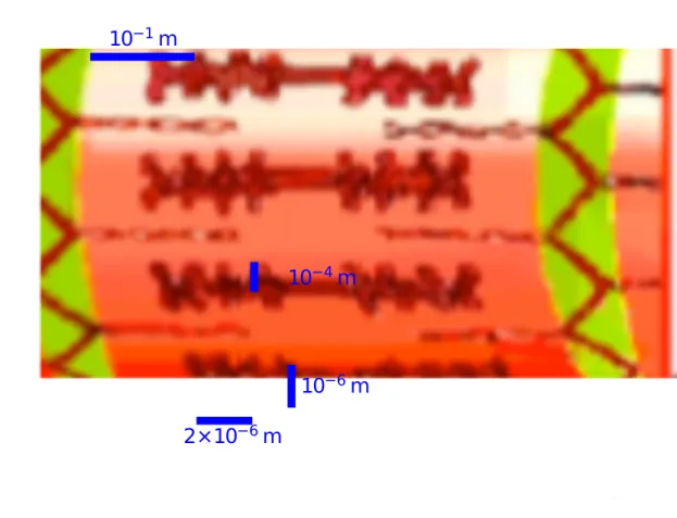
Skeletal and cardiac muscle are called striated muscle; this name is due to their striated appearance on the cell scale that is observed with microscopy. These striations are generated by the organized arrangement of protein filaments inside the muscle cell. A schematic representation of the structure of skeletal muscle is shown in Fig. 1.2.

The skeletal muscle fascicle is a bundle of cells held together by connective tissue, through which blood vessels and nerves. run These cells are called muscle fibers or myofibers. They mostly extend all the way, from one tendon to the opposite. In the human skeletal muscle the myofibers reach lengths up to tens of centimeters. They have a cylindrical shape with a diameter of ∼ 50µm. A muscle may comprise thousands of cylindrical myofibers.

The myofiber is a multi–nucleated cell. Its plasma membrane is called the sarcolemma, while the cytoplasm is known as the sarcoplasm. A large number (∼ 1000) of myofibrils are situated within the sarcolemma. Myofibrils extend to

(13)

10−1m

10−4m

10−6_m

2×10−6m

Figure 1.2: Schematic representation of a human biceps at various length scales.

the same length of the myofiber, while being only about 1 micron in diameter. The nuclei are flattened and pressed against the inside of the sarcolemma. Other organelles like the mitochondria that are responsible for the aerobic respiration, are surrounded by the myofibrils(see Fig. 1.3).

Each myofibril is a chain of sarcomeres, the basic functional unit of muscle cells. The sarcomere has the same diameter of the myofibril (∼ 1µm) and extends over 2-4 µm. It is delimited by the Z–disks at its two ends. The sarcomere has a symmetric structure and its middle–line is called M–line. A myofibril from a human biceps may contain 100,000 sarcomeres.

Inside the sarcomere protein filaments are arranged in arrays. These filaments are collectively called myofilaments: thick and thin filaments and titin.

(14)

Figure 1.3: A section of a multinucleated muscle cell.

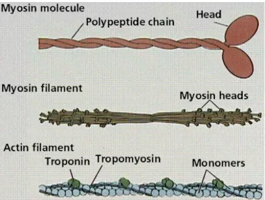
of the protein actin along with smaller amounts of two other proteins, troponin and tropomyosin. The actin filament (F–actin) is formed by polymerized G–actin units; it has a double helix conformation. The troponin is attached periodically on the actin filament. The tropomyosin, a protein of the length of one F–actin period, lies on the F–actin and is attached to the troponin (see Fig. 1.4). Troponin and tropomyosin are responsible for the regulation of activation (see Section 1.5). Two arrays of thin filaments are found in the sarcomere, one on each side of the M–line. The array of thin filaments is linked at one outer end to the corresponding Z–disk. The thick filaments have a diameter of about 15 nm, and are composed of myosin II protein (see Fig. 1.4). They are situated centrally in the sarcomere; at their center the filaments are connected together and form the M–line. Each thick filament is linked to the Z–disks by titin. Titin is one of the longest proteins known. Under normal conditions of contraction (sarcomere length up to 3.6 µm) it is slack and it tightens when the sarcomere length reaches its maximum extension. It is largely suggested that the main function of titin is to restrain the sarcomere from breaking off when overstretched.

(15)

Figure 1.4: Scheme of the thin and thick filaments.

The myosin II protein has three different domains: the heavy mero–myosin chain (HMM) also called myosin head, the light chain or neck domain and the tail (see Fig. 1.5). A myosin II motor unit is composed of two myosin proteins whose tails are interwind to form a single tail. The filament is obtained by many motor units whose tails twist to form a backbone; the myosin heads protrude from this backbone (see Fig. 1.4).

This arrangement of thin and thick filaments in the inner sarcomere is respon-sible for the striation of the muscle tissue observed with microscopy. In fact the dark band is due to the dense array of thick filaments, while the adjacent pale band corresponds to the array of thin filaments on each side of the Z–disk (see Fig. 1.2).

1.2 The muscle as an active tissue

The modern idea of how muscles operate was introduced in physiology by Helmholtz in 1848 [12]. He suggested that muscle dynamics is driven by the metabolism, i.e. chemical energy is consumed to perform mechanical work in much the same way as manmade machines do. Helmholtz’s purpose was to demonstrate the general validity of the law of conservation of energy. To prove his thesis, he performed

(16)

Figure 1.5: Schematic representation of the myosin II motor.

experiments on muscles of dead animals measuring the heat production during electrically stimulated contraction.

Helmholtz was followed by Heidenhain and Fick [2, 3], who made experiments on isolated frog muscles, mostly the sartorius, to investigate the heat–work rela-tionship in muscle contraction. Nevertheless, a satisfactory experimental basis of their hypothesis was furnished only by Hill and Fenn in the early 20th century [4,5]. These experiments were done on constantly activated muscle fascicle, i.e. under tetanus conditions. To obtain a tetanus, the muscle tissue was stimulated by an periodic electric signal. When stimulated, the muscle contracts and relaxes after a characteristic time. If the stimulation is repeated periodically the tension developed by the muscle is given by the sum of single responses. When the muscle is stimulated with an electric signal of frequency higher than a threshold (∼ 50 s−1), the muscle reaches constant activation (see Fig. 1.6).

(17)

Figure 1.6: Tension developed by muscle in response to electrical stimulation as a function of time. The different shapes correspond to stimulation with different frequencies. From left to right: at low frequency single twitches are measured; for increasing frequency a summation of tension is observed; even higher frequency produces an unfused tetanus, i.e. the muscle oscillates with constant mean value; finally, for frequencies beyond the threshold, the muscle reaches constant activation (fused tetanus).

Fenn realized a series of experiments to study the dynamics of isolated sartorius frog muscle. He found that the shortening heat, produced by the muscle during contraction, is roughly proportional to the work done, i.e. to the product of the length of shortening and the weight lifted. These observations were in contrast with the idea of muscle dynamics based on viscoelastic mechanisms, widely accepted at that time: the muscle was thought of as a pre–charged viscoelastic tissue. Fenn realized his experiments with the aim to disprove this current idea.

Today accurate experiments can be realized to measure the shortening heat and the relation between shortening heat and work was observed to depend on the particular type of muscle under exam (see [13] for a review).

1.2.1 Hill’s force–velocity relationship

Hill developed an experimental technique providing for a better time resolution in heat measures during muscle dynamics in tetanus conditions [4]. This technique allowed him to realize a systematic study of the temperature as a function of time during the contraction at constant activation and under isotonic conditions, i.e. with constant load attached to the muscle fascicle. Usually frog sartorius was used in these experiments. He did the following observations:

(18)

2. The temperature depend linearly on the amount of shortening.

3. The velocity of shortening and therefore the rate of heat absorbed depends on the weight muscle lifted by the muscle.

Hill deduced his famous force–velocity relationship from these results.

(P + a) · (v + b) = (P0+ a) · b = const, (1.1)

where P is the weight, v the velocity of shortening, P0 is the maximum load ( i.e.

a tetanus loaded with P0 will nor contract neither elongate), a is the rate of heat

produced during shortening a/P0 is a constant, b is a constant with the dimensions

of velocity. Although the force–velocity relationship was deduced by observations involving heat measures, the relationship itself does not depend on temperature and can be verified independently.

Figure 1.7: Schematics of the three–element model proposed by Hill.

Hill also proposed a model that represents an active muscle as composed of three elements. Two elements are arranged in series: a contractile element (CE) which at rest is freely extensible, but when activated is capable of shortening; and an elastic element (SE). To account for the elasticity of muscle at rest an elastic element (PE) was arranged in parallel to these serial structure (see Fig. 1.7) [14]. For the activated muscle the contractile element obeys the characteristic equation 1.1. The three–element model inspired various approaches on continuum muscle models [15, 16].

(19)

1.3 The mechanism of contraction

1.3.1 The sliding filament model

Figure 1.8: In the sliding filament model muscle contraction is generated at the sarcomere scale by the sliding of the thin filament with respect to the thick one toward the M–line.

An important interpretation of the microscope images of muscle tissue was given simultaneously and independently by Hanson and H.E. Huxley [17] and A.F. Huxley and Niedergerke [18]. In these two papers, published back–to–back in Nature, the observation of constant filament length during muscle contraction was discussed. Both groups presented the hypothesis of sliding filaments. In the sliding filament model, it is assumed that the shortening of muscle at the sarcomere scale is generated by the sliding of the thin filaments with respect to the thick ones (see Fig. 1.8); the intrinsic length of each filament will not change during contraction. In particular, A.F. Huxley and Niedergerke supposed point–wise interactions between the two contractile filaments. They proved that the isometric tetanus tension decreases with lengthening of the sarcomere and argued that the tension is produced proportionally to the overlap of the two filaments, actin and myosin.

In later works the relationship between sarcomere length and tension develop-ment was investigated [19–21] and the sarcomere–length relationship was estab-lished (see Fig. 1.9). This relationship can be well explained on the base of the

(20)

Figure 1.9: The sarcomere–length force relationship. The slope variates with qual-itative different arrangements of the filament couple of thick and thin filament inside the sarcomere.

sliding filament along with the point–wise interactions between the thick and the thin filament.

The sarcomere–length force relationship is piecewise affine, exhibiting four dif-ferent linear regimes that can be related to difdif-ferent overlap arrangements.

1.3.2 The Huxley cross–bridge model

A.F. Huxley published a very detailed review of experimental observations [6]. On this background, Huxley exposed a mathematical model to describe the sliding fil-ament dynamics generated by point–wise interactions. In the original model, these interactions are described by two different states, each state involving forces gener-ated by a harmonic potential, the dynamics being characterized by the transitions between these two states.

Huxley compared the results obtained from his model with those measured by Hill, i.e. force–velocity relationship and heat measurements produced as function of the contraction, finding an excellent agreement. The point–wise interactions between the two filaments were called cross–bridges and the model took the name of the cross–bridge model.

(21)

Schematic representation of the cross–bridge model

transition is much more rapid than the attachment and

detachment of the myosin head. This implies that these

two states are, e¡ectively, in equilibrium with each other,

although neither is in equilibrium with the detached state

D. The basic cycle involves binding of the myosin head at

rate f, which is quickly followed by the power stroke

tran-sition at a fast rate ¬. This puts the head in a

force-gener-ating, tightly bound state, from which it dissociates at rate

g. Detailed balance holds for each of these transitions, but

the corresponding changes of free energy are not known.

It is usual, however, to assume that one traversal of the

cycle is coupled to the hydrolysis of a single ATP

mole-cule, which puts a de¢nite constraint on the product of

the rates for all three transitions:

f £ ¬ £ g

f

_¡

¬

_¡

g

_¡ ˆ

exp

¢G

_ATP

k

_B

T

.

(4)

(c) Dynamics generated by many myosin molecules

In muscle, many myosin molecules act together to

cause the shortening of a sarcomere. As a simpli¢cation,

it is normal to consider the sliding of a single pair of

¢la-ments, caused by an ensemble of N molecular motors.

What methods can be used to calculate the overall

dynamics, given the basic mechanochemical cycle of an

individual cross-bridge outlined above?

The method that has been employed most extensively

follows the standard, ensemble-averaging approach of

statistical physics. One asks the following question: at a

given time, what is the probability that any myosin head

is in a speci¢ed biochemical state, with a particular value

of the strain? According to the kinetic scheme, general

equations can be written for the evolution of these

prob-ability distributions (Huxley 1957; Hill 1974). For

example, the equation for the detached state D in ¢gure 3

is

@p

_D

@t

_x‡

@p

_D

@x

_t

dx

dt

ˆ

f

¡

p

A1‡

gp

A2

¡ ( f

‡

g

¡

)p

D

.

(5)

In order to progress further, it is often necessary to make

further simpli¢cations. For example, to calculate the

rela-tionship between sliding velocity and applied load, it is

assumed that a steady state exists, in which the ¢laments

slide at a uniform speed v and the proportion of motors in

each state does not change with time. Then equation (5)

simpli¢es to

¡v

@p

D

@x

_t ˆ

f

¡

p

A1 ‡

gp

A2

¡ ( f

‡

g

¡

)p

D

(6)

and the full set of coupled equations can be solved to ¢nd

the steady-state probability distributions. The force

corre-sponding to this velocity can be obtained by integrating

the tension in the elastic elements of all of the motors:

F

ˆ

N

Z

‰ p

A1

(x)Kx

‡

p

A2

(x)K(x

‡

d)Šdx.

(7)

The advantage of this approach is that, once the probability

distributions have been obtained, many dynamic and

thermodynamic properties can be calculated from them.

The drawback is that it may overlook some important

physics, for there is no guarantee that a steady state exists

in all circumstances, as assumed. Indeed, the force^

velocity curve determined in this way really describes the

tension that is generated when steady shortening is

imposed, rather than the velocity of shortening under a

Kinetic models of linear motors T. Duke 531

A1 A2

D

f g

a

Figure 2. Basic cycle of the swinging cross-bridge model. The myosin molecule makes stochastic transitions between a detached state D, and two attached states, A1 and A2, which are structurally distinct. In general, the transition rates f, ¬, g and the corresponding reverse rates depend on the strain of the elastic element. Owing to the free-energy change

associated with ATP hydrolysis, the forward rates are

predominately faster than the reverse rates and the molecule is driven one way around the cycle: D!A1!A2!D. One ATP molecule is split during each cycle.

F F * F * d F * d/N_bound (a) F+Kd (b) F (c)

Figure 3. When a thin ¢lament of length L is propelled by N motor proteins, the typical time between chemical events is of the order or tchemˆ1/Nf. Each event perturbs the system

mechanically, and the time that it takes the ¢laments to adjust their position is of the order of tviscˆ²L/NK, where

²is the viscosity of the surrounding £uid. For a sarcomere, tvisc/tchemº 10¡2, so the ¢laments are in quasi-mechanical

equilibrium. (a) For a pair of ¢laments in mechanical equilibrium, the sum of the forces exerted by the motor proteins (grey arrow) is equal and opposite to the applied load (black arrow). (b) If one of the detached heads (marked with an asterisk) binds to the thin ¢lament and undergoes a power stroke transition, the ¢laments are momentarily out of equilibrium, owing to the additional force Kd exerted by this molecule. (c) As a consequence, the thin ¢lament slides leftwards through a small displacement Kd/N_bound, reducing the strain of all Nbound attached motors. Similar adjustments

occur when a head detaches, but the size and sign of the displacement varies according to the strain of the molecule immediately prior to dissociation.

Figure 1.10: The state A1 and A2 represent respectively the pre– and afterstroka, while D indicates the state of weak interaction. the transition rates between the three states are called f (D → A1), α( A1 → A2) and g (A2 → D). The interaction occurs cyclically.

The model was then extended to a three state model, today known as Huxley’s cross-bridge model [22]; the three states are the prestroke, aftersroke and the sate of weak interaction (see Fig. 1.10). This mathematical model inspired the the swinging lever arm model, a detailed model of the myosin dynamics at the nano– scale.

1.3.3 The swinging lever arm model

In the swinging lever arm model, the force transmitted through cross–bridge inter-actions is assumed to be generated by a conformational change of the light chain in the myosin protein (neck domain). The head domain is thought to exert a force on actin by the rotation of the myosin head, the neck domain having the role of lever arm (see Fig. 1.11). The chemical energy used by the myosin head to generate this force is obtained hydrolyzing AdenosineTriPhosphate (ATP) into AdenosineDiPhosphate (ADP) and Phosphor (P). The hydrolysis reaction occurs cyclically and the motor domain plays an enzymatic role in this reaction. The enzymatic reaction occurs when ATP adheres to the head domain of the myosin II protein.

(22)

Figure 1.11: Step 1: myosin attached to actin in its ground state. Step 2: ATP adheres to myosin, there is no more interaction between actin and myosin. Step 3: hydrolysis of ATP occurs, myosin absorbs the released chemical energy and acquires its excited, extended configuration. Step 4: myosin in its excited state reattaches to actin. Back to step 1: the excited state decays with the release of ADP and P from the head domain; myosin turns into the rigor state. During this conformational change it exerts a force on actin, causing filament to slide.

A simplified model of the ATP cycle is shown in Fig. 1.11. The cycle starts with an initial state 1 in which the ATP binding site on the myosin head is empty and myosin is strongly bound to actin. In muscle this state correspond to rigor mortis. When muscles are depleted of ATP, just after death, they become stiff and rigid, because without ATP, myosin heads stay firmly attached to thin filaments.

The ATP adheres to the myosin in the rigor configuration and myosin detaches from the actin filament. In this state there is no more interaction between actin and myosin. The head domain operates as an enzyme in the hydrolysis reaction (AT D → ADP + P ) and it absorbs the energy released during the hydrolysis.

(23)

Consequently, in step 3 of Fig. 1.11, the myosin head is in an excited state. In this state the neck domain forms a large angle with the filament, it is in an extended configuration. Myosin is now able to interact with actin. The next step occurs when myosin is bound to actin. Myosin is still in its excited state with extended configuration. The excited state decays when ADP and P are released from the head domain, myosin turns in its ground state at the low–angle configuration. During this conformational change myosin exerts a force on actin generating the sliding of the actin towards the center of the sarcomere (see Fig. 1.8).

The swinging lever arm model is a powerful tool to explain the contractile behavior of muscle tissue, since it predicts correctly numerous experimental obser-vations. However, there are experimental observation which cannot be explained within this framework [23, 24].

1.4 Experimental techniques on the nanoscale

Experiments are of great importance in muscle research and with the development of experimental techniques we get more and more details about the contraction mechanism.

In biology, experiments are classified as in vivo, in situ or in vitro. An in vivo experiment is realized on a part of a living organism without extracting it from the organism nor using invasive measurement techniques. In situ experiments are realized on systems which are situated in their natural environment, but, different to the in vivo experiments, in situ experiments are realized using invasive tech-niques, for example by mechanically manipulate the system under exam. Almost physiological conditions are guaranteed in this experiments. Finally, in in vitro ex-periments the system under exam is extracted from its physiological context and studied in an artificial environment controlled by the experimentalist.

The experiments on muscle mentioned in the previous sections of this chapter were all in vitro experiments. In this section, we introduce experimental techniques developed in the last 25 years to study biological systems at the nanoscale. Single molecule experiments are based on two key technologies: single molecule imaging and single molecule nano–manipulation. The difficulties in realizing experiments on systems at very small length scales are due also to the need of extracting minute

(24)

components of the muscle tissue without damaging them. Chemistry did a lot of progress on this issue, but it is beyond our scope to discuss that.

1.4.1 Single–molecule imaging

The imaging on very small length scale can be done by electron microscopy and X-ray diffractions. Both techniques are usually applied to solid materials. They are used to study crystallized single bio-molecules and small collective systems [25–27]. These techniques damage considerably the material under exam. In an interesting experiment the contraction dynamics of frog sartorius muscles tissue was visualized using X-ray diffraction [28, 29]. The authors were able to measure the fraction of attached cross-bridges in a small ensemble of myofibrils

Another technique to observe kinetic behavior at the nano scale is realized using fluorescence. FRET stands for F¨orster resonance energy transfer or fluorescence resonance energy transfer. This technique is used to measure the kinetics of single macromolecules of the nanometer size, such as large protein complexes. It takes advantage from the property of fluorescent molecules that absorb radiation of a given frequency ν and reemits radiation with frequency ν0 < ν. The technique involves two fluorescent molecules, a donor and an acceptor which were fixed on characteristic sites of the macromolecule under exam. The preparation of the protein is a challenge of molecular engineering.

The two fluorescent molecules, donor and acceptor, are chosen in such a way that the emission frequency ν_D0 of the donor overlaps with the absorption frequency νA of the acceptor. When emitting, the donor stimulates a nearby acceptor.

FRET is used to study configurational changes of the biomolecule by measuring the changes of the distance between donor and acceptor; it does not provide precise measurements of the distance between the marked zones on the macromolecule. The technique allows to measure spontaneous kinetics without the application of any force.

1.4.2 Micro–manipulation techniques

The single–molecule systems can be studied also using manipulation techniques. The dynamic response of biopolymers to external forces may shed light on

(25)

intrin-sic properties of the polymers itself. There are various techniques to manipulate biopolymers; mainly optical tweezers and the manipulation via microneedles is used to examine the piconewton forces exerted by molecular motors. A detailed description of two experiments realized with the optical tweezer is given in Chapter 3, where the experimental results are compared to computation; in Section 3.1 is described a single motor assay, while in Section 3.4is studied the response due to the interactions of a filament pair (actin and myosin).

By manipulating isolated bio-systems, the dynamics of single motors can be examined [7, 8, 30]. Advances in molecular engineering allowed to realize an exper-iment on myosin proteins with a modified length of their neck domain [31]. The response in displacement and force were measured for molecules with different neck size; the aim of the experiment was to proof the lever arm hypothesis in detail.

Filament systems constitute the level between single motors and sarcomeres. A pioneering experimental setup to test collective behavior was realized fixing a large number of myosin heads onto a glass plate and making an actin filament slide on them [9, 32, 33]. The actin filament is examined in different conditions, e.g. it drags a weight, or it is trapped by an optical tweezer. The kinetics of the filament can be measured and in the second case it can be measured the force that the filament exerts on the trap.

1.5 The mechanism of calcium control

The mechanism of regulation is of particular interest in studies of the cardiac muscle, as malfunction of the regulation in the heart muscle leads to death. Most physiological studies aiming at understanding the regulatory mechanisms are done on the cardiac muscle tissue. However, on the sarcomere level, cardiac and skeletal muscles are quite similar. As a consequence, I may give a description of the elementary molecular mechanism of Ca2+-regulation based on studies of both types of sarcomeres. Some known important differences between the two kinds of tissues are briefly discussed in Section 1.6.3.

Let us first introduce the main features of the regulatory structure on the thin filament [26, 34, 35]. The principal proteins involved in the regulation process are actin filament, troponin and tropomyosin (see Fig. 1.12). Actin monomers

(26)

CARDIAC THIN FILAMENT REGULATION 459 Tn-C

\

Tn-T1

ACTIN I

TROPOMYOSIN HEAD TO TAIL OVERLAP

OF TROPOMYOSIN

Figure3 Schematic representation ofa small region of the thin filament. The rabbit skeletal muscle TnT proteolytic fragment Tn-TI (residues 1-1 58) spans the tropomyosin-tropomyosin overlap joint. TnT fragment Tn-T2 (residues 159-259) interact with TnC and Tnl. (From Reference 62, with permission.)

(140, 174) and may extend through much of the considerable length of this molecule. However, the tertiary structure of TnT is unknown.

Interestingly, the globular head region of skeletal muscle troponin has an estimated dimension of 105 A (38), a value similar to the 115 8, span of the TnI-TnC complex in the Olah & Trewella model (129). TnT is rod-like and approximately 25

A

longer than the length of the tail in the ternary troponin complex (38). Evidently, the globular region consists of TnI, TnC, and a small portion of TnT. However, it is not clear what part(s) of the TnT sequence form the region interacting with the other two subunits. Tanokura et a1 reported that skeletal muscle TnT fragment 159-227 binds much more tightly to TnI than does TnT fragment 159-222 (174). Because the two fragments are similarly folded according to their circular dichroism spectra, the results suggest that TnT residues 223-227 are important for binding to TnI. Similarly, TnC Cys98 cross-links to TnT region 176230 (102) when all three subunits are present. In the binary TnT-TnC complex, TnT residues 175-178 are implicated. Chong & Hodges showed that Cys residues in the N-terminal region of TnI can be cross-linked to the 176-230 region of TnT (28). These studies can be summa- rized to implicate the 176230 region of skeletal muscle TnT as the primary site of interaction with the TnI-TnC complex. However, TnI cross-linking to Annual Reviews

www.annualreviews.org/aronline

Annu. Rev. Physiol. 1996.58:447-481. Downloaded from www.annualreviews.org

by Universita degli Studi Roma Tre on 09/28/10. For personal use only.

Figure 1.12: Schematic representation of the thin filament regulatory unit. The tro-ponin complex is composed of three subunits: trotro-ponin C, trotro-ponin I and trotro-ponin. The tropomyosin is made of monomers; two alpha-helix tropomyosin monomers dimerize to form a coiled structure that overlaps partially with the neighboring tropomyosin dimers to form a continuous tropomyosin strand. This strand lies in the two grooves of the F-actin double helix. Each tropomyosin dimer is bound on a troponin complex; the tail region of the troponin complex extends to the tropomyosin molecule at its overlap region with the neighboring dimer. Repro-duced from [34]

(globular actin) are polymerized into a double helical structure to form filamentous actin, the F-actin (see section 1.1). F-actin together with two tropomyosin strands, each binding a troponin complex, forms the thin filament. Tropomyosin and the troponin complex regulate the affinity of F-actin towards the myosin domains, i.e. they allow or inhibit the interaction between actin and myosin.One tropomyosin covers seven actin molecules, i.e. half the period of the actin helix. This entity is the regulatory unit of the thin filament.

Calcium ions adhere to the troponin complex and induce a structural change in troponin itself, which causes a relocation of the tropomyosin along the entire regulatory unit. Tropomyosin moves from its inhibitory position in the groove to a more peripheral position on the F-actin. In this way, the actin docking sites

(27)

are exposed to allow for interaction with the myosin domains [26]. There are very few single–motor assays performed on thin filament complete with their regulatory structure [36]. For this kind of experiment to be possible, the regulatory thin filament has to be reconstructed after the extraction of single proteins from the muscle tissue; this involves sophisticated chemical processes, difficult to realize.

1.5.1 The nervous stimulation in skeletal muscles

It is beyond the scope of this work to discuss extensively the whole mechanism of regulation from the muscle–fascicle scale down to a molecular motor. Nevertheless it is useful to have a general idea of muscle activation.

The skeletal muscle is stimulated by the somatic motor neurons. A neuron is composed the soma with the nucleus, dendrites and axons. The dendrites receive the nervous stimulus from other neurons forming a network while the axon connects the soma and the muscle cells. The extremes of the axon adhere to the muscle cell forming the synapse. The ensemble of cells (myofibers) activated by the same neuron forms what is called a motor unit. In the skeletal muscle, one motor unit confines to the next. At this border zone, the muscle cells of one motor unit are interspersed with cells from the confining motor unit. In this way, motor units take advantage of the contact forces to synchronize with neighboring units (see Fig.1.13).

The transport of the stimulus from the cell membrane to the interior of the cell is facilitated by the so-called T-tubules (see Fig.1.14). T-tubules form a dense network in the muscle cell: each sarcomere is surrounded by two T-tubules. The interior of the tubules is connected to the extracellular matrix; in other words, it is an extracellular space lined with a membrane. The activation potential generated by nervous stimulation is propagated across the surface membrane and down the T-tubules; this occurs mainly through currents of K+ _{and Na}+_{ions. Consequently,}

the voltage-mediated signal is transmitted to ryanodine receptors and induces the opening of calcium ion channels. These channels permit calcium to be released from the sarcoplasmic reticulum into the cytoplasm. Calcium ions are stored in the sarcolemma and when activation ends, they are pumped back there after a characteristic time.

(28)

Figure 1.13: Top: schematic representation of a single motor unit; the muscle cells are represented by cylinders and the axons by the lines connecting the cells. Bottom: schematic representation of the interspersed structure of the cells of two adjacent motor units.

(29)

Figure 1.14: Schematic representation of a couple of myofibril segments along with the sarcolemma and the structure of T-tubules. The T-tubules form a narrow network of channels in the muscle cell; geometrically the inside of the channels are connected to the extracellular matrix. T-tubules are important of the propagation of the nervous stimulus inside the muscle cell.

This propagation of the nervous stimulation requires an intact sarcoplasmatic reticulum, with T-tubules included. Therefore, stimulus activation can only be realized experimentally with intact muscle cells, not fortheir smaller parts. And infact, myofibrils need to be activated in a solution with a suitable concentration of Ca2+_.

1.6 Recent experiments and open questions

This section focusses attention on experimental research in muscle activation. This is a very broad field of research and an exhaustive discussion is beyond the scope of this work. I concentrate on three issues: the tetanization process, the phenomenon of force depression and force enhancement and the problem of myofibril length dependent activation.

(30)

1.6.1 The tetanization process

Tetanization is the process by which is obtained an intact muscle cell or a muscle fascicle in a constant activated state (see Section 1.2, Fig. 1.6). The tissue is stimulated by electric twitches of fixed constant frequency. This technique is well known and largely tested, as it is used since the end of the 19th century [2–5, 12]. If the twitch frequency is larger than a threshold frequency the muscle approaches constant tension exponentially in time [37].

Studies on the early stages of the tetanization process, the response to single twitches and the dependence of the contraction on the frequency of twitches provide insights of the muscle response to electric stimulation [38–41].

Moss [40] compared the response of intact muscle fibers excited to tetanus by twitches with the behavior of skinned fibers activated in a solution with a given calcium concentration. In particular, he compared chemically and mechanically skinned fibers. He found that the dynamics of the three differently treated fibers are indistinguishable, i.e. the response of the tissue was not influenced by the preparation of the fiber and the two ways of stimulation are equivalent.

Smaller units, like myofibrils, can only be activated by calcium ions in solution. Under the assumption that the extraction of a myofibril from muscle tissue does not alter qualitatively its behavior, experiments on myofibrils can reasonably be considered to give insights to the mechanism of activation on the nanoscale.

1.6.2 Force depression — force enhancement

The interest in activation studies increased with the progressive understanding of the contraction mechanism. In fact, as we saw in Section 1.1, Hill’s model and A.F. Huxley’s model give a description of the contractile behavior under constant activation and stationary force. To describe the response of the muscle tissue to a time-varying stimulus a mechano-electric feedback relation is required. The idea of a feedback relation was mentioned by Julian [20]. To shed light on this coupling various sophisticated experimental setups were designed which examines the length-dependent activation [29, 42–46].

This paragraph discusses the force depression assays. It was observed by several groups that the steady-state isometric force following shortening of an activated

(31)

muscle is smaller than the corresponding steady-state force obtained for a purely isometric contraction at the corresponding length [47–49]. This phenomenon is referred to as force depression.

!"#$%&'(&%)$&+)#$",%#%-&)(.&/%#%!"#%0&12&

,%)+3#'(4&'(.'5'.3)6&+)#$",%#%&6%(4/*+0&7%&

$)(&.%/%#,'(%&!"#$%&.%8#%++'"(&!"#&'(.'5'.3)6&

+)#$",%#%+9&

RESULTS AND DISCUSSION

&

:66&%6%5%(&,2"!'1#'6+&+*"7%.&!"#$%&

.%8#%++'"(&)5%#)4'(4&;<9=>;9?@&"!&/*%&

'+",%/#'$&#%!%#%($%&!"#$%&A!'43#%&<B9&

! "! #!! #"! $!! $"! %!! ! $! &! '! (! !"#$%&'( ') *$ ' ' %& + ,-.# /(

&&

**Figure 1. C2"!'1#'6&#%+8"(+%&7*%(&)$/'5)/%.&**

)/&)(&)5%#)4%&DE&"!&F9G!,0&/%(&+"#/%(%.&/"&

)(&)5%#)4%&DE&"!&F9H!,0&.%)$/'5)/%.0&/*%(&

)$/'5)/%.9&:##"7+&'(.'$)/%&/*%&)$/'5)/'"(&/',%9&

&

I'+&#%+36/&'(.'$)/%+&/)/&/*%&"#'4'(&"!&!"#$%&

.%8#%++'"(&,3+/&1%&7'/'(&/%&+)#$",%#'$&

+/#3$/3#%9&J(&"#.%#&/"&/%+/&'!&!"#$%&.%8#%++'"(&

,'4/&1%&$)3+%.&12&/%&.%5%6"8,%(/&"!&

+)#$",%#%&6%(4/*&("(K3('!"#,'/'%+0&7%&

/#)$L%.&+)#$",%#%&6%(4/*+&8#'"#&/"0&.3#'(4&)(.&

)!/%#&,2"!'1#'6&+"#/%('(49&:$$"#.'(4&/"&/%&

+)#$",%#%&6%(4/&("(K3('!"#,'/2&/%"#20&7%&

7"36.&%M8%$/&)(&'($#%)+%&'(&/*%&+)#$",%#%&

6%(4/&.'+/#'13/'"(&)!/%#&+"#/%('(4&)(.&)(&

)1"6'+*,%(/&"!&!"#$%&.%8#%++'"(&'(&'(.'5'.3)6&

+)#$",%#%+9&N"7%5%#0&/'+&7)+&("/&/%&$)+%9&

O'#+/0&+)#$",%#%&6%(4/+&)!/%#&+"#/%('(4&7%#%&

("(K3('!"#,&A/*%&+/)(.)#.&.%5')/'"(&ADPB&"!&

/%&+)#$",%#%&6%(4/+&7)+&=9<=!,B&13/&/*'+&

("(K3('!"#,'/2&7)+&("/&4#%)/%#&/)(&/%&("(&

3('!"#,'/2&"1+%#5%.&1%!"#%&+*"#/%('(4&ADPQ&

=9<F!,-&!'43#%&FB0&"#&/*%&("(K3('!"#,'/2&

"1/)'(%.&)/&F9H!,&)!/%#&/*%&83#%62&'+",%/#'$&

#%!%#%($%&!"#$%&ADPQ&=9<<!,B9&D%$"(.0&)66&

'(.'5'.3)6&+)#$",%#%+&A(QR=B&+*"7%.&!"#$%&

$)! $)$ $)& $)' $)( %)! ! " #! #" $! $" %! !"#$%&'( 01% &! #(

&

**Figure 2. D)#$",%#%&6%(4/*+&8#'"#&/"0&.3#'(4&**

)(.&)!/%#&+*"#/%('(4&!#",&)&/28'$)6&,2"!'1#'69&

&

I'+&#%+36/&+344%+/+&/)/&!"#$%&.%8#%++'"(&

$)(("/&1%&%M86)'(%.&12&/%&+)#$",%#%&6%(4/&

("(K3('!"#,'/'%+9&T)(4%+&'(&/%&L'(%/'$+&"!&

$#"++&1#'.4%+&6%).'(4&/"&)&.%$#%)+%&'(&/*%&

!"#$%&8#".3$%.&8%#&$#"++&1#'.4%&"#&/*%&(3,1%#&

"!&)//)$%.&$#"++K1#'.4%+&+"36.&1%&

$"(+'.%#%.9&J/&)+&1%%(&8#"8"+%.&AC)#%$)6&

)(.&U6)4L'0&<?V?B&/)/&+"#/%('(4&,'4/&

'(.3$%&)(&'(*'1'/'"(&"!&$#"++K1#'.4%&

)//)$,%(/&'(&/%&(%762&!"#,%.&"5%#6)8&W"(%&

)(.&/%#%!"#%&#%+36/'(4&'(&)&.%$#%)+%&'(&/%&

(3,1%#&"!&)//)$*%.&$#"++K1#'.4%+&)(.&!"#$%9&&

CONCLUSION

&

O"#$%&.%8#%++'"(&."%+&("/&.%8%(.&"(&

+)#$",%#%&6%(4/&("(K3('!"#,'/20&13/&#)/%#&

+%%,+&)(&'(%#%(/&8#"8%#/2&"!&/%&,"6%$36)#&

,%$*)('+,&3(.%#62'(4&$"(/#)$/'"(9&

REFERENCES

&

:11"//0&XT&)(.&:31%#/0&YC&A<?SFB9&J.

Physiol&<<VZVVKGR9&

[.,)(&\

&%/&)69&A<??;B9&J Physio6&HRRZS;SKSSF9&

N%#W"40&]&)(.&E%"()#.0&I^&A<??VB9&J

Biomech&;=ZGRSKGVF9&

C)#%$)60&_&)(.&U6)4L'0&E&A<?V?B9&J Gen

Physiol&V;ZHS;KHRV9&

C"#4)(&PE&%/&)69&AF===B9&J Physiol&SFFZS=;K

S<;9&

ACKNOWLEDGEMENTS

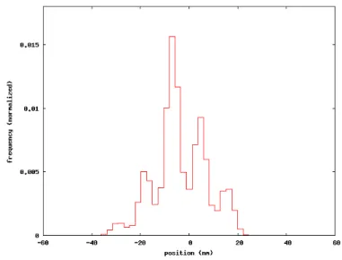
O"#$%& .%8#%++'"(& *+,-$)(!.- *+,-$)&!.-*+,-$)&!.

Figure 1.15: Myofibril response in tension during activation at an average sarcom-ere length (SL) of 2.8µm. The fibril is shortened to an average SL of 2.4µm. After more than 60s the fibril is deactivated and reactivated under constant SL (2.4µm). Reproduced from [50]

Joumaa and Herzog performed an experiment to test force depression in my-ofibrils of rabbit psoas muscle [50]. Isolated mymy-ofibrils from rabbit psoas muscle were fixed to a glass needle on a motor at one end and to a nanolever at the other end, allowing for length changes and force measurements, respectively. The myofibril is activated through the concentration of calcium ions in the flow cell. The activation is held constant and the length is modified, from 2.8µm to 2.4µm average sarcomere length (see Fig. 1.15). During this process of shortening the stress decreases. After tens of seconds in which the stress of the myofibril re-main constant, the tissue is deactivated and then reactivated after a few seconds. The stress developed after the reactivation is bigger than the initially developed stress at 2.8µm average sarcomere length. The difference of the stresses at 2.4µm, i.e. the difference of the stress obtained respectively before and after the de- and reactivation, measures the amount of force depression (see Fig. 1.15).

In particular Herzog’s group studied this phenomena at various length-scales; force depression was observed from the single myofibril up to the entire muscle fascicle [50, 51].

Analogously to force depression, also force enhancement was observed when the

(32)

muscle was stretched under constant activation [52]. It was suggested that the mechanisms on the molecular scale generating force enhancement is similar to that generating force depression. The origin of both phenomena is still unclear. One of the hypotheses proposed to explain force depression is sarcomere length non-uniformity. According to this hypothesis, during shortening on the descending limb of the force-length relationship, sarcomeres are assumed to shorten by different amounts because of instability. Some sarcomeres do nearly not shorten, whereas others shorten more than average; these sarcomeres may shorten to a degree that places them on the ascending limb of the force-length relationship. This behavior leads to a situation in which the tension produced is smaller than that produced at the corresponding length during an isometric contraction in which sarcomere lengths are assumed to be relatively uniform. Another hypothesis is set forth by Herzog’s group. They suggest that force depression is due to history dependence of contraction, i.e. the behavior of the muscle tissue depends on its initial mechanical and electrical state [44, 53].

1.6.3 Length–dependent activation

Calcium regulation of muscle tissue is observed to depend on the sarcomere length [35, 45, 54]. The conjecture that Ca2+ _{sensitivity is due to changes in the}

spac-ing between the thick and thin filaments is responsible for this dependence was largely accepted [55]. It was supposed that the sarcomere maintains constant vol-ume during contraction and therefore, it was expected that the spacing between the thin and thick filaments decreases with lengthening of the sarcomere. On the molecular level this conjecture is explained as follows: when getting closer to actin myosin heads may have an increased probability of strong cross-bridge formation. Sophisticated experimental techniques were improved, in which myofibrils are com-pressed via the osmotic pressure that is obtained by adding dextran to the flow-cell solution. Several experiments have provided some support to this theory [56, 57].

A more recent experiment on cardiac myofibrils, realized by de Tombe et al. [58], discredited this hypothesis bringing forward the idea that activation depends on the tension of myofilaments. The authors realized a comprehensive series of experiments, concluding that the decrease of inter–filament distance might not be

(33)

the primary mechanism generating length–dependent activation. Moreover, the authors suggest that the molecular mechanisms that underlie this phenomenon are governed by structural and functional modulation of the sarcomere proteins which depends directly on the sarcomere length. Many different underlying mechanisms — some of them involving titin — could produce this result and I am not going to discuss them all here. The one I am interested in is related to calcium. The length–dependent activation might be governed by cooperative binding of calcium along the thin filaments, sensitive to the filament tension itself and hence to the sarcomere length. A possibility to model this cooperative binding is to introduce a sarcomere length dependent correlation length for calcium binding along the actin filament. Further experimental work has to be done to shed light on this issue.

The phenomenon outlined in this section is of great interest in cardiac muscle research although it is observed also in skeletal muscle [59]. A brief description of similarities and differences between skeletal and cardiac muscle tissue is given in the following.

In skeletal muscle, individual myocytes are fully activated via motor nerve ac-tivity. Thus, muscle force is mainly tuned via motor unit recruitment. In contrast, the cardiac muscle is activated by calcium–induced calcium release mechanism: the electrical stimulation readily spreads via low resistance gap junctions. All striated muscle, skeletal and cardiac, are fundamentally the same, i.e. the same type of proteins make up the sarcomere, but they differ in terms of the specific isoforms expression of these proteins. This may explain the greater myofilament length-dependent activation observed in cardiac muscle with respect to skeletal muscle.

1.6.4 ADP–regulated activation

It is worth noting that activation is observed even in absence of calcium ions. In this case, activation is generated by an ADP concentration in the flow-cell solu-tion [60,61]. In recent years, experiments on ADP activasolu-tion where put forward and particular interest was given to the spontaneous oscillations (SPOC) observed [62]. SPOC were first observed in calcium activated muscle [63]. It was even realized a single–motor experiment in which ADP-induced activation was tested [36]. An

(34)

intact thin filament was reproduced by combining the F-actin with the regulatory proteins, troponin and tropomyosin. In this work, the following conjecture was made to explain the mechanism of ADP-induce activation at the molecular level. It was suggested that fluctuations of the tropomyosin strand occur due to Brown-ian motion. These spatial fluctuations are responsible for partial exposition of the docking site on the actin filament. Therefore, rare events are possible in which the myosin domain can bind actin, even when troponin is not activated. A high ADP concentration induces strong binding between actin and myosin, so that these rare events have a greater probability to occur. Once the actin-myosin binding has occurred, tropomyosin is moved to a peripheral location by the attached myosin domain. All the docking sites belonging to this regulatory unit become exposed to interaction with myosin and strong bonds are favored by the high ADP concen-tration. In conclusion, activation has taken place.

This scenario on the nanoscale is in agreement with the model dynamics I consider here. Under the above assumptions on the molecular mechanisms, ADP regulation goes along with the exposition of the docking sites just like the effect of the acti-vation through calcium ions. We may imagine that ADP-actiacti-vation will not reach the tetanus level, but maybe low activation. Indeed, SPOC were first observed in myofibrils for activation through low calcium concentration [45,63].This conjecture is also in agreement with the experimental observation of SPOC for activation by low calcium concentrations. In conclusion, we may say that ADP-activation is roughly equivalent to activation through low concentrations of calcium ions.

(35)

Chapter 2 Modeling muscle contraction at

the nanoscale

2.1 Classification of molecular motors

On the nanoscale the mechanism of muscle contraction is driven by the Myosin II molecular motor. Many different kinds of molecular motors exist with different roles. They are important for the functioning of cells and different approaches were developed to study them. In this section, I give an overview on molecular motors, mainly to characterize the muscle motor.

Definition of molecular motors Molecular motors are biological molecular ma-chines that convert the chemical energy derived from the hydrolysis of ATP into mechanical work. In the ATP-hydrolysis reaction they have an enzymatic role, they induce the hydrolysis reaction without changing their own chemistry. Molec-ular motors operate in the thermal bath, an environment where fluctuation due to thermal noise are significant.

Transverse and rotatory motors Many different kind of motors exist in nature. Motors can be distinguished in transverse and rotatory with respect of the kind of motion they generate. Rotatory motors are found to manage the selective perme-ability of the cell membrane via channels and ion pumps for example. Transverse motors are responsible for the transport, muscle contraction, and deformation of the cell. Three different families of transverse motors are known: kinesin, dynein,

(36)

myosin; kinesin and dynein move along tubuli, while myosin acts on the F-actin. Porters and rowers Transverse molecular motors have two active domains, they can be classified in porters and rowers [64]. Porters are called the motors that never get completely unbound from the supporting protein, respectively the mi-crotubules or the actin. The motor protein has two active domains and at least one of them is attached to the support. Porters move stepwise along the partner protein. Contrary, rowers may be completely unattached from the supporting pro-tein, even if they have two active domains. The myosin II motor in the muscle is a rower.

2.2 Modeling molecular motors

Molecular motors are of the dimension of ∼ 10 nm, their dynamics cannot be observed directly. Micromanipulation experiments allow for the measurements of displacement and force generated by a single motor or collective motor system (see Sections 3.1 and 3.4). Modeling molecular motors is a tool to interpret and inspire the indirect measurements of motor behavior. To this end, models were designed on various length scales. To choose between them the modeler has to evaluate which model better correspond to the aim of his or her work.

Detailed models may describe more directly the biophysical states during hy-drolysis. This kind of models have the advantage to consider a big number of information about the fine mechanism and they may work for a lot of different situations. On the other hand these models are characterized by a large number of parameters, which are not easy to fix, because experimental data does not yet exist to well constrain the rate constants and parameters.

Contrary, simplified, coarse models are based on very few parameters to be set. This is a great advantage, because they are less arbitrary and parameters can be better constrained with experiment. These models will lack of generality because they do not go into the details of the mechanism, the simplicity may preclude versatility and extensibility to other applications.

The best compromise is given by the model that requires the minimum mech-anistic detail needed to recapitulate the phenomena of interest. In the following

(37)

some examples are given for different approaches.

Molecular motors move in biological systems where they are surrounded by a thermic bath. It is widely assumed that the thermal energy has a crucial role in motor dynamics. In a coarse model, the motor can be described as a Brownian particle.

The theory of Brownian motion was formalized by Einstein and Langevin at the beginning of the 19th century [65–68], it describes a particle suspended in an isothermal solution. The motor protein is some order of magnitude bigger than the molecules in solution (∼ 0.1 nm), therefore the hypothesis of scale division required to observe Brownian motion is verified. The motion of the Brownian particle is described by the Langevin equation.

The motor consumes energy to generate force, this is modeled by introducing an interaction potential between the motor and the supporting protein in the Langevin equation. The potential energy is characterized by at least two different states; the transition between the two states is designed to furnish the system with chemical energy (ATP-hydrolysis-cycle).

2.2.1 Coarse cross–bridge models

There are mainly two different approaches to model the energy transfer, the cross– bridge model and the Brownian ratchet. In the cross–bridge model at least three states are distinguished, two states with strong interaction (pre and after–stroke) and one weakly bound state (see Section 1.3.2, Fig. 1.10). The weakly bound state represents the free state, in which actin and myosin do not interact, while the attached state before the power stroke and after the power stroke correspond to the strongly bound pre and after–stroke states. In every state the potential energy is given by a harmonic function, the stiffness of the strong bound states are greater than the stiffness characterizing the weakly bound state. The equilibrium position changes from the pre–stroke to the after–stroke state; the power stroke is modeled by the transition between these two states. The transition between the states is determined by the transition rates which generally depend on the motor position.

(38)

of molecular motors, representing a filament. He supposed strain dependence of the transition rates and a suitable compliance to allow for the interaction of many motors contemporarily. Duke confronted the response of a system of 50 filaments linked in series with the experimental results of velocity as a function of load, the results were in excellent agreement. Hence, the coarse model reproduces suc-cessfully experimental results obtained for tetanized myofibrils directly from the filament setup, without considering the parallel system of filaments in the sarcom-ere. Further, averaging the dynamics of many filaments dragging a certain load, Duke found stepwise movement for loads near to the isometric load. In this lat-ter numerical experiment the filaments are supposed to be independent from each other.

Other approaches were setting forth, e.g. the discrete master equation is used to implement the cross–bridge model [70], a review can be found in [71].

2.2.2 Brownian ratchet models

The model of the thermal ratchet was first introduced by Feynman [72]. The model is characterized by a sawtooth potential and under the condition of a thermal gra-dient the ratchet produces force. In isothermal conditions, the ratchet is not able to produce force; energy has to be pumped in the system. The model was extended to allow for energy supply through chemical reactions, at least two different chem-ical states are necessary: an interactive state and a free state or even two well chosen interactive states. Muscle motors can be modeled considering an interac-tive and a free state, they represent respecinterac-tively the attached and the unattached state of the motor domain. The cyclic transition between these states represent the ATP-hydrolysis. This modified ratchet is called Brownian ratchet, for review see [73–78].

The Brownian ratchet is studied for an unbounded number of motors which are characterized by a distribution function. Shimowaka et al. [79] calculated analyt-ically the Gibbs free energy and the net displacement as a function of transition rates for an unbounded ensemble of motors under stationary transition conditions. The authors used a three state Brownian ratchet whose states were chosen similar to the three states of the cross–bridge.

(39)

Also an analytical approach to bounded ensembles of motors was set forward by Gaveau et al. [80]. Another contribution to the characterization of Brownian ratchet models was given by J¨ulicher et al. [1, 81]. The behavior of unbounded ensembles of motors was characterized in the stationary state. Non–trivial behavior was found for a two–state Brownian ratchet, e. g. spontaneous oscillations were observed in certain ranges of the transition rates, and further, spiral motion was found in two dimensions. These characteristics seem to be appropriate to describe the oscillations in insect flight muscles or the movement of actin in the cytoskeleton respectively.

The two–state Brownian ratchet was also integrated numerically. In this case, the system comprises a bounded number of linked motors moving on the same support [82]. The response was studied comparing an asymmetric potential shape with a symmetric one. For the symmetric sawtooth potential and under load the system shows bidirectional motion, i.e. it inverts velocity unexpectedly. The same behavior was not found for the asymmetric sawtooth potential. This phenomenon is observed experimentally for collective systems of transverse porter–like motors, e.g. kinesin.

2.2.3 Towards detailed models

To understand the fine mechanism of motor activity more detailed models are designed. Obviously there is no clear cut between coarse and detailed models. Here, I consider a detailed model, the model which does not focus only on the very fundamental dynamic functions of the motor but aim to comprehend for molecular or chemical details. This model is always a coarse model with respect to the atomistic length–scale.

Recent work is done on models combining coarse models with molecular simu-lation [83–85]. The attempt is to overcome the lack of parameters determined by experiment by ab initio simulation and the aim is to shed light on the molecular mechanism of motor mechanics. Another approach is to model details of the chem-ical transitions during the hydrolysis cycle. To this end, the cross–bridge model is used and further internal states are introduced in the system to describe the APT-hydrolysis. [86–88].

(40)

2.3 The 1D two state model

In this thesis, we are interested to investigate the role of active proteins in the activation process of muscle tissue. The tissue is intended to be a macroscopic portion at least at the micro-scale, i.e. the sarcomere scale. The sarcomere is composed of thousands of thin and thick filament pairs, each filament pair has hundreds of motors on the thick filament. To model a huge collective system a Brownian ratchet coarse model is chosen.

I suggest that the filament setup (serial motors) and the sarcomere setup (par-allel filaments) is important to the dynamics under partial activation. Hence, the single motor system will be extended to these two types of collective systems. The simplicity of the model allows for a good control on the model parameters; nearly all model parameters have a direct physical interpretation.

Further my aim is to extend the model to allow for varying activation. The sim-plest mechanism of activation is a switch–like mechanism that can be conceptually easily introduced in the ratchet model (see Section 4.1).

2.3.1 Interaction potential and equations of motion

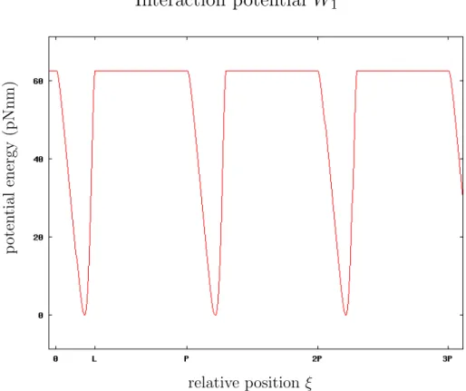
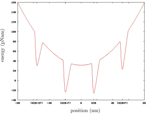
The 1D model, I set forth in this work, describes the dynamics of the myosin II motor on actin and is based on the two state ratchet model [1]. One molecular motor is composed of two bodies, respectively the myosin head and the actin filament. The myosin head is regarded as a point-like particle, while the actin filament is represented by a massless rigid rod. The interaction potential between the two bodies describes the interaction due to the activated docking sites on the actin filament.

The system is described by the positions of myosin (x) and actin (y) and its internal chemical state s. The internal state can take two values, corresponding to two different chemical states of the myosin domain during the hydrolysis cycle: (1) interacting, and (2) non-interacting with the F-actin.

The interacting state represents myosin in its ground state (state 1 in Fig. (2.1)), attached to the actin filament, in this state the myosin exerts mechanical force on actin. The latter, non-interacting state is given by the excited myosin head along with ADP and P (step 4 in Fig.(2.1)), here, myosin do not interact

A simplified 1D model for the chemo-mechanical coupling in sarcomere dynamics

SCUOLA DOTTORALE IN FISICA

XXII CICLO