UNIVERSITÀ CATTOLICA DEL SACRO CUORE
Dipartimento di Economia e Finanza
Working Paper Series
Does fiscal decentralization affect regional
disparities in health?
Quasi-experimental evidence from Italy
Cinzia Di Novi, Massimiliano Piacenza, Silvana Robone, Gilberto Turati
Working Paper n. 83 July 2019
Vaccination take-up and health:
evidence from a flu vaccination program
for the elderly
Cinzia Di Novi
Università degli Studi di Pavia
Massimiliano Piacenza
Università degli Studi del Piemonte Orientale
Silvana Robone
Università degli Studi dell’Insubria
Gilberto Turati
Università Cattolica del Sacro Cuore
Working Paper n. 83
July 2019
Dipartimento di Economia e Finanza Università Cattolica del Sacro Cuore Largo Gemelli 1 - 20123 Milano – Italy tel: +39.02.7234.2976 - fax: +39.02.7234.2781
e-mail: [email protected]
The Working Paper Series promotes the circulation of research results produced by the members and affiliates of the Dipartimento di Economia e Finanza, with the aim of encouraging their dissemination and discussion. Results may be in a preliminary or advanced stage. The Dipartimento di Economia e Finanza is part of the Dipartimenti e Istituti di Scienze Economiche (DISCE) of the Università Cattolica del Sacro Cuore.
Does fiscal decentralization affect regional disparities in health? Quasi-experimental evidence from Italy
Cinzia DI NOVI *§
Massimiliano PIACENZA + # §
Silvana ROBONE †§
Gilberto TURATI ° §
Abstract
Recent theories on fiscal decentralization support the view that sub-national governments who finance a larger share of their spending with taxes raised locally by themselves are more accountable towards their citizens. Whilst evidence on improvements in spending efficiency is relatively common, little is known about the effects on inequalities amongst the population. In this paper we exploit a reform aimed at increasing regional tax autonomy in Italy to provide quasi-experimental evidence on the impact of fiscal decentralization on health disparities between- and within-regions. Our findings, robust to a number of robustness checks, support the view that fiscal decentralization does not impact on between-regional inequalities but can help to reduce inequalities within regions. However, this last effect depends on the degree of economic development: richer regions are better than poorer ones in containing inequalities.
JEL codes: H75, I14, I15, I18, R50
Keywords: fiscal decentralization, regional governments, healthcare policy, health inequalities
* University of Pavia – Dept. of Economics and Management, Via San Felice 5, 27100 Pavia, Italy. E-mail:
§ Health Econometrics and Data Group (HEDG), University of York, Alcuin Building, Heslington, YO10 5DD,
York, UK.
+ Corresponding Author: University of Piemonte Orientale – Dept. of Economics and Business (DISEI), Via
Perrone 18, 28100 Novara, Italy. E-mail: [email protected].
# Italian National Research Council – Research Institute on Sustainable Economic Growth (CNR-IRCrES), Via
Real Collegio 30, 10024 Moncalieri (TO), Italy.
† University of Insubria – Dept. of Economics, via Monte Generoso 71, 21100 Varese, Italy. E-mail:
Bocconi University – Dondena Centre for Research on Social Dynamics and Public Policy, via Roentgen 1,
20136 Milano, Italy
° Catholic University – Dept. of Economics and Finance, Largo Francesco Vito 1, 00168 Roma, Italy. E-mail: [email protected].
1. Introduction
The transfer of political power and fiscal resources to sub-national tiers of government has been traditionally justified on identity grounds and heterogeneous preferences across jurisdictions (e.g., De Winter and Tursan, 1998; Oates, 1999). More recently however, a different argument has been proposed to support decentralization, namely that (fiscal) decentralization creates incentives for local officials that make them more accountable towards their citizens, hence improving the performance of their jurisdictions (e.g., Bardhan, 2002; Weingast, 2009).
While the theoretical literature is unanimous, empirical evidence is less supportive. For instance, critics point out that decentralization can lead to an increase in both the size and the number of bureaucracies (e.g., Reverte-Cejudo and Sánchez-Bayle, 1999; Repullo, 2007), and additionally to an uneven geographical distribution of benefits (e.g., Martınez-Vazquez and McNab, 2003). However, the empirical literature on the impact of decentralization on inequality is relatively scarce and provides mixed results (e.g., McKinnon, 1997; Qian and Weingast, 1997; Cheshire and Gordon, 1998; Shankar and Shah, 2003; Gil et al., 2004; Rodriguez-Poze and Ezcurra, 2010).
The distributional concerns become particularly apparent when considering specific policies. In this paper we concentrate on health care, and ask what are the consequences of fiscal decentralization on health disparities. The decentralization of health policy responsibilities is quite common around the world, even in unitary states (e.g., Saltman et al., 2007; Costa-Font and Greer, 2013). The central government typically devolves political authority to sub-national governments, who can then autonomously legislate on health care issues and decide how to spend monies (political and spending decentralization). But it can also assign fiscal autonomy to lower-tier governments, by granting them independent sources of revenue to finance the provision of services (fiscal decentralization).
Our focus is on the Italian National Health Service (NHS). The NHS was established in 1978, replacing the previous system based on insurance funds, with the declared goal of improving equity by providing uniform and comprehensive healthcare services across the country. However, healthcare expenditure increased steadily over time, and at the beginning of the 1990s the central government introduced reforms aimed at capping spending growth. These reforms shifted the responsibility of both managing and funding the services towards regional jurisdictions. Their declared aim was to improve spending
efficiency by increasing regional governments’ accountability via fiscal autonomy (e.g.,
Bordignon and Turati, 2009; Ferrario and Zanardi, 2011; Piacenza and Turati, 2014).
However, some scholars have questioned the overall welfare consequences of decentralization, which – despite improving efficiency – might have sharpened the existing differences in the access and quality of care across regions. In particular, critics point out that the richest regions could exploit substantial tax bases after devolution, and then spend more. As a consequence, between-regional inequalities might increase, and welfare in poorer regions might decrease.
But this argument fails to take into account that in Italy, as in other countries, fiscal decentralization has come together with (i) equalization grants to substantially remove differences in the tax bases, and (ii) constitutional rules defining a mandatory uniform provision of a quasi-universal set of services across the country (e.g., Costa-Font and Turati, 2017). As a consequence, following fiscal decentralization, the relative distribution of resources across regions should remain substantially stable, but the composition of funding across those same regions could change significantly. In particular, rich regions should be increasingly financed with more autonomous sources of funds1. And, according to both the
theoretical and the empirical literature on fiscal federalism, the lower the share of transfers from central government sources to finance local spending, the higher will be the accountability of local officials (e.g., Weingast, 2009; Eyraud and Lusinyan, 2013).
What are the consequences on health disparities of increasing the share of local taxes to finance regional health spending? In this paper we assess the impact of fiscal decentralization of health care funding on between- and within-regional disparities in self-assessed health. Weexploit a reform increasing fiscal autonomy of Italian regions since 1998 which had clear and substantial consequences on the composition of funding (e.g., Eyraud and Lusinyan, 2013, Fig. 4). The regional setting of the Italian NHS and the wide variation in the size of the tax bases offer a unique opportunity to this end. Our main finding suggests that fiscal decentralization helped contain health disparities within more fiscally autonomous regions, in a period in which within-region health inequalities were on the rise. According to our estimates, the impact on the inequality index has been on average about three times its within-region standard deviation, with much stronger effects in richer regions compared to poorer ones. This result has been obtained without any major effect on between-regional health disparities and without decreasing average perceived health.
1 The gap between sub-national government’ own revenue and spending identifies in the literature on fiscal
Our work is related to the growing literature studying the impact of decentralization on a variety of health outcomes, which provides empirical results that are often mixed and inconclusive (e.g., Jepsson and Okuonzi, 2000; Tang and Bloom, 2000; Bossert et al., 2003; Akin et al., 2005; Arreondo et al., 2005; Kolehmainen-Aitken, 2005; Saltman et al., 2007; Jimenez-Rubio, 2011; Jimenez-Rubio and Garcia-Gomez, 2017). In work considering the Italian NHS, most have focused on the relationship between decentralization and the efficiency of health policies, providing strong support to the argument that fiscal decentralization makes local governments more accountable (e.g., Bordignon and Turati, 2009; Francese et al., 2014; Piacenza and Turati, 2014; Cavalieri and Ferrante, 2016). As for the impact on inequalities, studies available so far (not only in economics) have discussed the between-regional dimension of disparities, finding mixed evidence on the impact of decentralization (e.g., De Belvis, 2012; Toth, 2014; Blöchliger et al., 2016; Costa-Font and Turati, 2017).
The remainder of this paper is organized as follows. Section 2 provides essential background information on the fiscal decentralization reform. Section 3 provides descriptive evidence on the impact of the reform on the outcome of interest. Section 4 presents the empirical strategy. Estimates are discussed in section 5, while section 6 provides brief concluding remarks.
2. Institutional background: fiscal decentralization in Italy
The Italian NHS is a regional system designed according to the Republican Constitution (e.g., Turati, 2014). Regional governments have the right to legislate on the organization and the supply of health care services and to allocate spending, albeit this right is limited by the legislative framework set by the central government.2 Particularly important, in this respect,
is the definition of a quasi-universal set of services to be offered across all territories. This provision limits the autonomy of regional governments to enlarge the set of services publicly provided3. However, it also facilitates the comparison of access and quality of
services locally supplied across different regional governments.
2 Regions are the level of government directly below the central government, and above provinces and
municipalities. There are 20 regions in Italy, and they vary widely in terms of size, population, and per-capita GDP. Five of these regions historically enjoy a Special Statute, meaning they are allowed a higher degree of autonomy.
3 A striking example is dental care, which is only marginally included in the set of services identified by the
central government to be provided across all regions. None of the regional governments have used the available degree of fiscal autonomy to supply their citizens with this service, likely because the costs involved would be too high even for rich regions.
According to independent reviewers, the Italian health care system is one of the best performers at the global level.4 However, this good performance at national level hides
important differences across regions, and there is unequivocal evidence showing a deterioration in the performance of regional health care systems, moving from the North to the South of the country (e.g., Turati, 2014). For instance, the Ministry of Health carries out a yearly evaluation exercise to verify whether regional governments are effectively supplying the set of services constitutionally guaranteed. The evaluation is based on a set of indicators which are summed to obtain a final score; if the score is above a given threshold, then it is assumed that the regional governments fulfill the Constitutional mandate. Since the beginning of this exercise in 2001, most of the Southern regions have been unable to reach the minimum threshold required.5
The gradient in regional performances mirrors differences in income: the Italian
Mezzogiorno – the Southern part of Italy – is poorer than the Northern part of the country.
The persistently uneven distribution of income across regions had striking consequences when – during the Nineties – the central government reformed NHS funding, to match political and spending decentralization with fiscal decentralization. The main motivation behind the reform was to increase accountability at the local level (e.g., Eyraud and Lusinyan, 2013). Theory predicts that greater accountability would have been obtained by reducing transfers from the central government. In turn, more accountability would have produced an improvement in spending efficiency. To pursue this aim, following a first attempt in 1993, in 1998 the central government substituted transfers from the centre with two new autonomous sources of revenue for regions: a new regional tax on value added (IRAP), and a regional surcharge on the Personal Income Tax (Addizionale Regionale IRPEF). The reason for substituting transfers with own revenues was to exploit the potential gains of decentralization while respecting the constitutional provision of uniform levels of care to be guaranteed by the central government in all regions. As transfers from the central government were cut by an amount equivalent to the increase in autonomous revenues for all regions, the reform did not modify the relative amount of resources for each region’s budget for health (which increased over time), but it did change differently for different regions the composition of funding according to the tax base available in each jurisdiction.
4 See, e.g.,
http://www.bloomberg.com/infographics/2014-09-15/most-efficient-health-care-around-the-world.html.
5 See, e.g., the most recent official report (in Italian) published by the Ministry of Health at
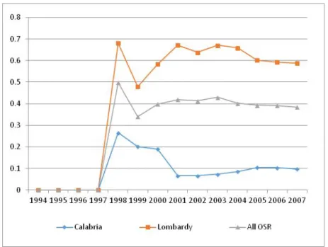
To understand the magnitude of the impact, consider Figure 1, where we plot the share of healthcare spending financed by IRAP and IRPEF. At the national level, this share is around 40% of total spending. However, since income is unevenly distributed across regions and the tax bases of the two new regional taxes are strictly positively related to GDP, the impact of the decentralization reform on fiscal autonomy was also unequal. In Lombardy, the richest region, IRAP and IRPEF cover as much as 60% of spending; in Calabria, the poorest region, the two new taxes fund about 10% of spending. In general, richer Northern regions experienced a larger reduction of transfers with respect to Southern regions, who continued to mostly rely on grants from the centre to fund healthcare spending. Own revenues represent about half of revenues in Centre-Northern regions, while they are just 15% in Southern ones (e.g., Turati, 2014). As theory predicts, changes in the efficiency of health spending management were also estimated to be different across regions, with efficiency in Northern regions increasing more than in Southern ones (Bordignon and Turati, 2009; Piacenza and Turati, 2014; Cavalieri and Ferrante, 2016).
Figure 1. Share of healthcare spending financed with regional taxes
3. Data and preliminary descriptive evidence
In order to obtain regional measures of inequality we consider individual-level data drawn from the 1994–2007 cross-sectional Survey on the Daily Life of Italian Households (“Indagine
Institute of Statistics (ISTAT).6 The survey encompasses a sample of 20,000 Italian
households (60,000 individuals) living across Italy, and is representative of the whole population.7 We limit our analysis to those over 16 years old living in one of the 15
Ordinary Statute Regions.8
Self-assessed health (SAH) is our indicator for general health. SAH has been widely used in the literature examining the relationship between health, socio-economic status and life-styles (e.g., Kenkel, 1994; Contoyannis and Jones, 2004; Balia and Jones, 2008). Moreover, SAH has been shown to be a good predictor of mortality and morbidity (e.g., Idler and Beyamini, 1997; Kennedy et al., 1998), and to have a strong correlation with more complex health and well-being indices (e.g., Unden and Elofosson, 2006). As in other similar surveys around the world, respondents are asked the following question: “Would you say that in general your health is: very bad (1), bad (2), fair (3), good (4), very good (5)”.9 SAH is clearly
measured on an ordinal and categorical scale, and it requires appropriate statistical tools for the analysis.
We begin our analysis by briefly discussing the evolution of between-regional inequality. Table 1 shows some descriptive statistics on the development of SAH across all regions, before (1994-1997) and after (1998-2007) the fiscal decentralization reform. For both the median value of SAH and the percentage of individuals responding having “good” and
6 Data concerning 2004 are not included in the analysis since the survey did not take place. We also do not
consider data after 2007 since the incentive mechanism stemming from fiscal decentralization was substituted by centralized Recovery Plans for regional governments in deficit. Additionally, ISTAT changed the wording of the question on self-assessed health in 2008.
7 As common when using individual survey data, we use survey stratification weights provided by ISTAT in
all our models. Survey stratification weights are defined during survey sampling by the provider of the data and are essential to make the analysis representative of the entire population.
8 Special Statute Regions in the North and in the South have been excluded because they follow different rules
and are characterized by different degrees of fiscal autonomy. Interestingly, the inclusion of these regions in the sample strengthen our main conclusions. Results obtained for the full sample of Italian regions are briefly discussed in section 5.2 and do not affect our main conclusions.
9 Notice that when individuals are faced with an instrument comprising ordinal response categories, their
interpretation of response categories may systematically differ across populations or populations sub-groups, also depending on their preferences and norms (Bago d’Uva et al., 2008; Rice et al., 2012). In such cases a given level of health is unlikely to be rated equally by all respondents. This phenomenon has been termed “reporting heterogeneity”. In order to check that reporting heterogeneity is not a relevant issue for our analysis, we have computed the correlation between self-reported health and a more objective indicator of health, constructed through responses to fairly precise questions about specific health conditions. To build this summary measure, we use the number of health conditions reported by the respondents during the interview (heart problems, high blood pressure, high cholesterol, stroke, diabetes, lung disease, asthma, arthritis, osteoporosis, cancer, ulcer, Parkinson disease, cataracts, hip or femoral fracture, psychological problems). For each year, we run an ordered probit regression model in which the independent variable is SAH and the
dependent variable is the summary indicator of health conditions. The adjusted R2 of the model tends to be
constant and equal to about 15% for all years. Hence, SAH appears as strongly predictive of the summary health index. Moreover, the results of a chi-square test shows a large and statistically significant correlation between the two variables, since, for each year, their correlation coefficients tend to be constant and equal approximately 60%.
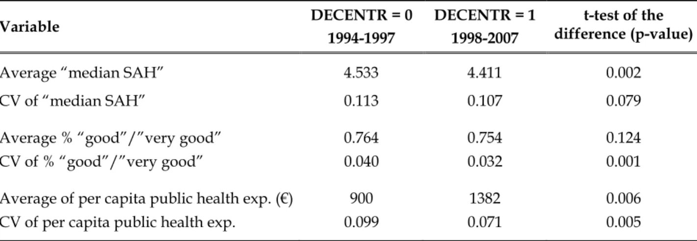
“very good” health, we compute the mean and the coefficient of variation (CV) across regions for the two sub-periods. Neither measure shows substantial changes over time; but more importantly, the between-regional disparities in health outcomes (as measured by CV) decreased slightly. This evidence confirms the view that the tax decentralization reform has not exacerbated health disparities between regions, largely because a system of equalization grants was implemented (e.g., Costa-Font and Turati, 2017). It is also worth noting that the average per capita public health expenditure significantly increased by roughly 500 euro after the reform, while the coefficient of variation across regions slightly decreased, thus revealing also a reduction in between-regional disparities in health spending.
Variable DECENTR = 0 1994-1997 DECENTR = 1 1998-2007 t-test of the difference (p-value)
Average “median SAH” 4.533 4.411 0.002
CV of “median SAH” 0.113 0.107 0.079
Average % “good”/”very good” 0.764 0.754 0.124
CV of % “good”/”very good” 0.040 0.032 0.001
Average of per capita public health exp. (€) 900 1382 0.006
CV of per capita public health exp. 0.099 0.071 0.005
Table 1. Average and coefficient of variation (CV) across regions of health outcomes and per capita public health expenditure in the years before and after the reform
In order to provide a more detailed view of the dynamics of health outcomes across regions, Figures 2a and 2b show the evolution of the median value of SAH and the percentage of individuals responding having “good” and “very good” health over the years from 1993 to 2007 respectively. In each figure, we present the average across all regions (green line), and the averages across the sub-samples of regions with (average) per-capita GDP below and above the sample mean value (“low-GDP” regions, red line; “high-GDP” regions, blue line). Figure 2a shows that median SAH is generally constant over time, with a very slight decrease in both the high- and low-GDP regions. In 1993, the average median SAH is 4.2 and 5 for the high-GDP and low-GDP regions respectively, while in 2007 it is 4 and 4.7 for the high-GDP and low-GDP regions respectively. Interestingly, the average median value of SAH in the low-GDP (high-GDP) regions is always above (below) the national average. More importantly, the distance between the low-GDP and high-GDP regions in terms of median SAH is quite stable across the time span considered, which further supports the
view that health disparities between regions did not increase after the tax decentralization reform. A similar pattern is found for the evolution of the percentage of individuals reporting “good” and “very good” health (Figure 2b).
Figure 2a. Average median value of SAH, by year
Figure 2b. Average % of individuals reporting “good”/“very good” health, by year
Turning now to within-regional variation in SAH, we make use of the innovative inequality index developed by Kobus and Milos (2012), a generalization of the Abul Naga and Yalcin (2008) index. The KM inequality index is “median based” (and not “mean based” as the
3 4 5 5. 5 a v er a g e m e di an S A H 1993 1995 1998 2000 2005 2007 year
high-GDP Regions low-GDP Regions all Regions .6 5 .7 .7 5 .8 .8 5 ave rag e % go od /v e ry g o o d 1993 1995 1998 2000 2005 2007 year
high-GDP Regions low-GDP Regions all Regions
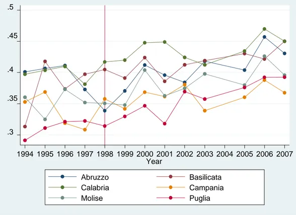
more traditional inequality indexes) and lies in the interval [0, 1]. The average value of the KM index (computed using symmetric weights for inequalities below and above the median) across regions and years is approximately 0.4 (Table 2), relatively high in comparison to other European countries studied in the still limited literature using median-based inequality indexes.10 Figures 3a and 3b illustrate the evolution of the KM index over
the period 1994-2007 for low-GDP regions (the less fiscally autonomous, Figure 3a) and for high-GDP regions (those more fiscally autonomous, Figure 3b). It is difficult to gauge a common pattern, but health inequalities in the first group of regions seems to increase after the fiscal decentralization reform, whereas inequality in the second group of regions appears relatively stable across the whole period.
This suggests that higher fiscal autonomy is associated with reduced inequality and we now turn our attention to identifying this relationship using a formal econometric model.
Figure 3a. KM index in regions with per-capita GDP below the mean, by region and year
10 For instance, Abul Naga and Yalcin (2008) estimated an average level of inequality in self-assessed health
across seven regions in Switzerland of 0.208. Madden (2010) reported an inequality index in SAH ranging from 0.356 in 2003 to 0.333 in 2006 for Ireland.
.3 .35 .4 .45 .5 1994 1995 1996 1997 1998 1999 2000 2001 2002 2003 2004 2005 2006 2007 Year Abruzzo Basilicata Calabria Campania Molise Puglia
Figure 3b. KM index in regions with per-capita GDP above the mean, by region and year
4. The empirical strategy
4.1. Identification
In order to investigate the impact of the fiscal decentralization reform on within-regional health inequalities measured by the KM index, we exploit the differences in the level of income across the Italian regions. In particular, regions characterized by a higher per-capita income – hence, a higher tax base for the two new sources of own revenue – have become more fiscally autonomous than regions with a lower per-capita income (Figure 1)11. And, in
turn, this would have made local politicians more accountable towards their citizens in rich regions than in poor ones. We exploit between- and within-regional variability in current GDP and adopt a multivalued treatment approach (e.g., Imbens and Wooldridge, 2009). Our general model specification is the following:
KMit = Ri + Tt + βGDPit×DECENTRt + Xit’δ + it [1]
11 We do not consider revenues from IRAP and IRPEF since these would clearly suffer a problem of
endogeneity. .3 .35 .4 .45 .5 1994 1995 1996 1997 1998 1999 2000 2001 2002 2003 2004 2005 2006 2007 Year
Emilia Romagna Lazio
Liguria Lombardia
Marche Piemonte
Toscana
Umbria Veneto
where KMit is our inequality measure in Region i at time t; Ri denotes a full set of
region-specific effects, Tt denotes a full set of year-specific effects, Xit is a vector of controls, and it
is a disturbance term. Standard errors are robust, clustered at the regional level to capture potential serial correlation in the residual error term, in all estimated models.
The average causal impact of the tax decentralization reform is captured by the coefficient β on the interaction term GDPit×DECENTRt, where DECENTRt is a dummy equal to 0 in the
pre-reform period and equal to 1 from 1998 onwards. Our identification strategy relies on two assumptions. First, the degree of exposure to treatment (GDP) should be conditionally uncorrelated with the outcome variable (KM). This means assuming that current GDP is orthogonal to the current level of inequality in perceived health, once controlling for time and regional fixed effects as well as a number of additional covariates. However, despite this specification, one might be worried that inequalities in health reflect inequalities in income, and that these inequalities in health are (negatively) correlated with the level of GDP. In the robustness section below we address this concern by using a pre-treatment variable as an exogenous alternative measure of the degree of exposure.
A second key assumption for the validity of our identification strategy is that the outcomes in regions differently exposed to treatment follow the same trend before the reform takes effect. As suggested by a large literature in econometrics (e.g. Angrist and Pischke, 2009), in order to test the common trend assumption, one can augment a standard difference-in-differences (DiD) regression model to include leading values of the treatment variable. If such leads were associated with the outcome variable, it would indicate that our results might be due to time trends in regions in the treatment group being systematically different from time trends in regions in the control group. The practice of including anticipatory effects in a DiD regression model to test the validity of the common trend assumption is widespread among health economics scholars (e.g. Wing et al., 2018) and may be easily accommodated in our multivalued treatment framework. 12 In the analysis below, we then
augment Eq. [1] with a full set of anticipatory effects (leads) of the treatment. When using this augmented specification of Eq. [1], we also considerpost-treatment effects (lags) to test whether the impact of the reform was delayed over time.
Finally, a potential problem with the linear model specification we adopt is that it may not be a good representation of the data generating process for a variable assuming only values
12 For instance, this practice is adopted by Bachhuber et al. (2014) when studying the relationship between
medical cannabis laws and opioid overdose mortality, and by Raifman et al. (2017) when investigating the relationship between same-sex marriage laws and adolescent suicide attempts.
between [0, 1] as the KM inequality index, since fitted values might stay outside the relevant interval (e.g., Wooldridge 2002). To support the robustness of our model specification, we then check whether fitted values of the inequality index from the estimated models are bounded in the interval [0, 1].
4.2. Confounding factors
Controls Xit in equation [1] include several confounding factors which may vary both across
regions and over time. In particular, we consider two main groups of covariates: a) measures of within-regional inequality in healthcare services utilization and in lifestyles; b) regional demographic and socio-economic characteristics.
Both the use of healthcare services and lifestyles have been recognized as important determinants of inequality in health (e.g., Mackenbach, 2012, 2014). To build suitable inequality measures in these two dimensions, we exploit additional information at the individual level provided by the ISTAT Multiscopo survey. In particular, we consider four measures of inequality in services utilization: home care (inequality_home_care), emergency care (inequality_emergency_care), inpatient care (inequality_inpatient_care), and contacts with Local Health Authority to schedule appointments for outpatient visits, blood tests or other laboratory tests (inequality_contacts_LHA). All of these inequality measures are built from binary variables indicating whether or not the respondent had used any of the services during the twelve months before the interview. To account for the binary nature of these variables, we use the concentration index proposed by Erreygers (2009) to build our measures of inequality. The Erreygers index E(y) corrects the standard concentration index defined by Wagstaff et al. (1991) and Wagstaff and Van Doorslaer (2000).13 The range of the
Erreygers index E(y) is [−1, 1]. A negative (positive) value indicates a pro-poor (pro-rich) inequality; a value of zero indicates that healthcare access is perfectly equally distributed among the population. Since we are interested in the magnitude of need-adjusted horizontal inequality in healthcare access, we employ the absolute value of the index.
13 Notice that, differently from the standard concentration index, the Erreygers index does not depend on the
mean of health, healthcare and health-related behavior variables. This makes it possible to compare regions with different averages. Moreover, while the standard concentration index may give conflicting information when applied separately to health and ill-health, the Erreygers index satisfies the so called ‘‘mirror property’’, namely inequalities in health ‘‘mirrors’’ those in ill-health (Erreygers et al., 2012; Costa-Font et al., 2014). Further notice that, since straightforward numeric measures of wealth such as household income are not available in the ISTAT survey, we have to use other proxies for the household wealth. In particular, we exploit information about assets ownership and living standards collected during the interviews to build a one-dimensional index of wealth using the Principal Component Analysis (PCA), under the assumption that wealth is reflected in the assets owned and in the living conditions within a household. For a detailed discussion of how to construct asset indices see Vyas and Kumaranayake (2006).
Moreover, we standardize utilization considering need factors related to the individuals’ health status.14
Although the role of access to healthcare services in addressing health inequality is widely recognized, there is an additional concern about growing differences in lifestyles (e.g., Costa-Font et al, 2014; Mackenbach, 2014; Vallejo-Torres et al., 2014). While there exists a substantial literature that shows that a healthier lifestyle is one of the main driving factors for good health (e.g., Contoyannis and Jones, 2004; Balia and Jones, 2008; Di Novi, 2010), little is known about the potential influence that these inequalities in lifestyles may have on health inequality. In our study we consider two measures of lifestyle differences: an index for differences in diet (inequality_diet) and an index for differences in smoking
(inequality_smoke).These inequality measures are built from individual level variables
provided by the ISTAT Multiscopo survey. As for diet, we use a binary variable that takes value one if the respondent does not eat breakfast nearly every day and zero otherwise.15 To
measure smoking behavior we also employ a binary variable that takes value one if the respondent is currently a smoker and zero otherwise. Following Costa-Font et al. (2014), to account for the bounded nature of the health-related behavior variables (between 0 and 1), we again apply the Erreygers (2009) index. Additionally, in order to have a measure of lifestyle differences reflecting only non-demographic factors, we use the indirect method of standardization discussed above. Finally, as before, since we are interested only in the magnitude of differences in unhealthy habits, regardless of the sign (pro-poor or pro-rich), in the final regression model we include the absolute value of the two lifestyle-related indexes.
Table 2 shows that inequalities in healthcare access are pro-poor and close to zero, except for contacts with Local Health Authority to schedule appointments, which tends to be
14 In other words, instead of using the actual measure of healthcare access, we consider a “corrected” measure
accounting for differences in needs. To this end, we start by estimating a probit model controlling for the determinants of healthcare access for each region and for each year survey. We categorize the explicative variables used to predict the demand for healthcare services into three main dimensions: need factors related to individuals’ health status (age, gender, self-assessed health and health conditions), social characteristics (education and marital status), and enabling/disabling factors (private health insurance, employment status, wealth, difficulties in accessing healthcare services due to distance, monetary costs, or waiting times). We then standardize access by need factors related to individuals’ health status to obtain an estimate of potentially avoidable inequality (see also O’Donnell et al., 2008). The standardisation allows for exploring whether lower socioeconomic groups are less likely to access healthcare than higher socioeconomic groups, keeping needs constant. After standardisation, any residual inequality in healthcare access is interpretable as horizontal inequity (which could be pro-rich or pro-poor).
15 Belloc and Breslow (1972) in their epidemiological study based on the Alameda County survey carried out
in California in 1965, found that people who eat breakfast almost every day reported better overall physical health status than breakfast skippers.
rich. Looking at the dynamics of the indexes during the observed period, inequalities tend to increase over time, especially for regions with GDP per-capita below the sample mean value, which generally present greater inequality in access even when pro-poor.16
Consistent with the previous literature, differences in unhealthy lifestyles also appear to be concentrated among the poor and tend to be higher in poorer regions over time.
Demographic and socio-economic characteristics at the regional level, and summary information on regional health policies, are other important variables which may influence the inequality in health status and are included in Xit. To control for these factors, we use
data at the regional level from the ISTAT “Health for All - Italy” database. In particular, in our econometric model we control for variables capturing: (i) demographic characteristics of the regional population, namely the percentage of individuals older than 65 (population_over65) and the percentage of foreign-born residents (population_foreign); (ii) disposable income, namely the percentage of low educated individuals (population_primaryedu, the share of population with at most a primary school certificate according to ISCED classification) and the employment rate (population_employment, the share of individuals older than 15 who were employed during the year of the interview)17;
(iii) the consumption rate of prescription drugs (drug_consumption, the share of individuals who consumed drugs in the two days before the interview); and (iv) the level of public health expenditure per-capita (health_spending).
Summary statistics for all variables included in the estimated models are in Table 2. Approximately 20% of the sample are over 65, and only about 2% are foreign-born. The percentage of people with a low level of education is relatively small (about 28%), while more than 40% of individuals were employed during the year of the interview. Approximately one in three consumed drugs within two days before the interview, and the average public health expenditure per-capita is around 1200 euro over the whole sample period.
16 Descriptive statistics for inequality indexes disaggregated by years and regions are not reported for sake of
brevity but are available on request.
17 These two variables will serve as proxies for private health spending, which cannot be included directly
Variable Mean Std. Dev. Min Max KM index 0.399 0.031 0.291 0.470 GDP (€) 19,801 5748 9072 33,122 DECENTR 0.692 0.463 0 1 inequality_home_care -0.009 0.015 -0.054 0.054 inequality_emergency_care -0.010 0.021 -0.078 0.062 inequality_contacts_LHA 0.028 0.058 -0.121 0.297 inequality_inpatient_care -0.012 0.016 -0.054 0.030 inequality_diet -0.013 0.029 -0.130 0.064 inequality_smoke -0.013 0.046 -0.142 0.138 population_over65 (%) 19.345 3.121 12.090 26.740 population_foreign (%) 2.313 1.815 0.280 7.590 population_primaryedu (%) 28.170 16.327 0.363 46.930 population_employment (%) 42.918 5.924 31.590 53.270 drug_consumption (%) 34.720 4.806 24.750 45.320 health_spending (€) 1234 326 694 2014 Nr. Observations 195
Table 2. Summary statistics of the variables used in model [1]
5. Results
5.1. Baseline results
Table 3 shows the estimated impact of fiscal decentralization on within-regional health inequalities under alternative specifications of Equation [1]. All of these specifications include the set of possible confounding factors Xit, regional fixed effects Ri, and year fixed
effects Tt, to account for unobserved residual heterogeneity across regions as well as the
presence of a common time trend.18 MODEL 1 refers to the baseline specification of
equation [1], without any controls for possible anticipatory effects (leads) or post-treatment effects (lags). MODELS 2 to 5 test the robustness of the baseline results by including q leads and m lags of the treatment. More precisely, following Angrist and Pischke (2009), all the models account for three anticipatory effects (GDP×1 Year Prior = 1997, GDP×2 Years Prior = 1996, GDP×3 Years Prior = 1995). As for the lags, MODEL 2 includes only one post-treatment
18 As anticipated in section 3, we have verified that the fitted values of the inequality index from the estimated
models stay inside the interval [0. 1]. This is the case for all the specifications presented in Table 3, with values ranging from 0.328 to 0.463. Our linear model appears to be an acceptable representation of the data-generating process.
effect (GDP× 1 or More Years After = 1999-2007); MODEL 3 includes two post-treatment effects (GDP×1 or More Years After = 1999, GDP×2 or More Years After = 2000-2007); MODEL 4 includes three post-treatment effects (GDP×1 or More Years After = 1999, GDP×2 or More
Years After = 2000, GDP×3 or More Years After = 2001-2007); MODEL 5 includes four post-treatment effects (GDP×1 or More Years After = 1999, GDP×2 or More Years After = 2000,
GDP×3 or More Years After = 2001, GDP×4 or More Years After = 2002-2007). Finally, in all the models GDP×Year of Adoption refers only to the effect of tax decentralization observed in
1998, when the reform was implemented.
Regressors MODEL1 MODEL2 MODEL3 MODEL4 MODEL5
GDP×DECENTR -2.160** (0.847) - - - -
GDP×3 Years Prior - -3.005 (2.822) -3.592 (2.820) -3.490 (2.845) -3.670 (2.950)
GDP×2 Years Prior - -2.231 (1.941) -2.963 (1.920) -2.817 (1.929) -3.022 (2.047)
GDP×1 Year Prior - -2.091 (2.617) -2.982 (2.598) -2.871 (2.614) -3.013 (2.707)
GDP×Year of Adoption - -3.289 (2339) -4.347* (2.237) -4.174* (2.249) -4.409* (2.357)
GDP×1 or More Years After - -5.059* (2.453) -3.887* (2.172) -3.697 (2.201) -3.996 (2.330)
GDP×2 or More Years After - - -7.253** (2.444) -7.623*** (2.570) -7.947** (2.730)
GDP×3 or More Years After - - - -6.729** (2.458) -6.429** (2.228)
GDP×4 or More Years After - - - - -7.449** (2.970)
Within R2 0.48 0.49 0.52 0.52 0.53
Nr. of observations 195 195 195 195 195
Table 3. The impact of fiscal decentralization on health inequalities (a)
(a) The dependent variable is the index of inequality in self-assessed health (KM). Cluster–robust standard errors at the Region level are reported in round brackets. All models include the vector of control X, regional and year FE. MODEL 2-5 extend the baseline specification to include leads (GDP×1 Year Prior = 1997, GDP×2 Years Prior = 1996, GDP×3 Years Prior = 1995) and lags (GDP×1 or More
Years After refers to time period 1999-2007 in MODEL 2 and only to year 1999 in MODELS 3-5; GDP×2 or More Years After refers to
time period 2000-2007 in MODEL 3 and only to year 2000 in MODELS 4-5; GDP×3 or More Years After refers to time period 2001-2007 in MODEL 4 and only to year 2001 in MODEL5; GDP×4 or More Years After refers to time period 2002-2007). GDP×Year of Adoption refers only to the effect of decentralization observed in year 1998.
**statistically significant at 5%; *statistically significant at 10%.
The estimates in Table 3 show that the different specifications provide a consistent picture. Looking at MODEL 1, the coefficient on the interaction GDP×DECENTR is negative and statistically significant. Given the evolution characterizing within-regional inequality, this means that the tax decentralization reform helped contain disparities within regions. As discussed above, this result might hide differences in pre-trends and/or in post-treatment effects that are not controlled for in the baseline model. However, looking at the extended
specifications (MODELS 2-5), coefficients for the three leads are always statistically insignificant, supporting the common trend assumption underlying our empirical strategy. In all the models except MODEL 2 the estimated coefficient for the year of adoption of the reform (GDP×Year of Adoption) is negative and statistically significant. More importantly,
coefficients for the lags reveal that the magnitude of the impact increases in the years after the introduction of the reform, supporting the idea that it takes time for the reform to completely generate its effects. In particular, the impact of the reform on within-regional health inequalities is almost two times larger after two years from its adoption (coefficient for GDP×2 or More Years After) and then remains fairly constant at this new level.
The Average Treatment Effect, computed at the sample mean value of GDP in the years from 1998 to 2007, points to a reduction in KM of almost three times its within-region standard deviation, computed over the same time period. The effect clearly differs according to the exposure to the treatment, with much stronger effects in richer regions compared to poorer ones. Looking at the two extreme cases for instance, the reform caused a reduction in KM which varies from about one and a half times the within standard deviation for the region with the lowest per capita GDP (Calabria, on average 14,238 euro over the period 1998-2007) to about six times the within standard deviation for the region with the highest per capita GDP (Lombardy, on average 29,272 euro). As the theory predicted, the decentralization reform had more pronounced effects in the regions that experienced a substantial increase in their fiscal autonomy; and these effects were not enough to contrast the increasing inequalities in poorer regions. This finding suggests that the increased accountability of regional governments was beneficial not only to foster efficiency, but also to avoid the deterioration of within-region inequalities.
As for the role played by the controls, results are also consistent across the different models, with most coefficients statistically insignificant.19 Of the six inequality indexes, only
inequality in home care is positively correlated – as expected – with KM, while we do not find evidence of statistically significant effects for the remaining variables. Looking at regional characteristics, the estimates show that KM increases with the consumption rate of drugs. This result might be due to the fact that the assessment of own health conditions is likely to be more heterogeneous within the group of drug consumers, in which there are both people who use drugs for minor ailments and people with serious diseases.
5.2. Robustness checks
Our results might be influenced by different important sources of bias. First of all, as discussed in section 4.1, the use of current GDP as a measure for the degree of exposure to treatment (DECENTR) can raise endogeneity concerns; secondly, some regions might have used deficits to inflate spending in health care, and this increased spending might have influenced health outcomes as well; thirdly, a reform impacting on the financing mechanism of hospitals – which deployed its effects since 2007 – might have produced better outcomes in richer regions. We consider all of these issues in turn. As a final check, we estimate all models additionally including Special Statute Regions in our sample, and compare the results with those obtained from estimations using the original sample of Ordinary Statute Regions.
Regressors MODEL1 MODEL2 MODEL3 MODEL4 MODEL5
PRE×DECENTR -2.950*** (0.753) - - - -
PRE×3 Years Prior - -2.611 (2.476) -2.673 (2.440) -2.660 (2.460) -2.724 (2.503)
PRE×2 Years Prior - -1.727 (1.611) -1.697 (1.637) -1.679 (1.651) -1.717 (1.672)
PRE×1 Year Prior - -1.549 (2.383) -1.632 (2.333) -1.675 (2.373) -1.652 (2.351)
PRE×Year of Adoption - -3.009 (1.996) -3.022 (1.910) -3.035 (1.950) -3.053 (1.962)
PRE×1 or More Years After - -4.951** (1.998) -2.488 (1.831) -2.470 (1.872) -2.551 (1.899)
PRE×2 or More Years After - - -5.816** (1.997) -6.790** (2.339) -6.815** (2.345)
PRE×3 or More Years After - - - -5.398** (1.943) -4.716** (1.708)
PRE×4 or More Years After - - - - -5.854** (2.317)
Within R2 0.47 0.49 0.51 0.52 0.52
Nr. of observations 195 195 195 195 195
Table 4. The impact of fiscal decentralization on health inequalities controlling for the potential endogeneity of contemporaneous GDP (a)
(a) The effect of the potential endogeneity of contemporaneous GDP is tested by defining the variable PRE as the average regional GDP over the pre-reform period 1994-1997. The dependent variable is the index of inequality in self-assessed health (KM). Cluster– robust standard errors at the Region level are reported in round brackets. All models include the vector of control X, regional and year FE. MODEL 2-5 extend the baseline specification to include leads (GDP×1 Year Prior = 1997, GDP×2 Years Prior = 1996, GDP×3
Years Prior = 1995) and lags (GDP×1 or More Years After refers to time period 1999-2007 in MODEL 2 and only to year 1999 in
MODELS 3-5; GDP×2 or More Years After refers to time period 2000-2007 in MODEL 3 and only to year 2000 in MODELS 4-5; GDP×3
or More Years After refers to time period 2001-2007 in MODEL 4 and only to year 2001 in MODEL5; GDP×4 or More Years After refers
to time period 2002-2007). GDP×Year of Adoption refers only to the effect of decentralization observed in year 1998. **statistically significant at 5%; *statistically significant at 10%.
We address the issue of the potential endogeneity of current GDP by utilising the average of regional GDP prior to the reform. In particular, we define the variable PRE as the average
regional GDP over the period 1994-1997. We then replace the variable GDP with the variable PRE in all models. The estimates of this new version of Eq. [1] are reported in Table 4 and largely confirm the baseline findings in terms of sign, statistical significance and magnitude of the impact of the reform, which suggests that our estimates are not biased by potential endogeneity of the treatment variable.
Regressors MODEL1 MODEL2 MODEL3 MODEL4 MODEL5
GDP×DECENTR -2.207* (1.266) - - - -
GDP×3 Years Prior - -4.000 (2.969) -4.602 (2.954) -4.526 (2.968) -4.684 (3.041)
GDP×2 Years Prior - -2.987 (2.253) -3.682 (2.227) -3.579 (2.219) -3.729 (2.270)
GDP×1 Year Prior - -2.271 (2.784) -3.175 (2.838) -3.093 (2.847) -3.208 (2.887)
GDP×Year of Adoption - -3.945 (2.647) -4.927* (2.491) -4.789* (2.483) -4.993* (2.549)
GDP×1 or More Years After - -5.825* (2.705) -4.734* (2.375) -4.583* (2.384) -4.844* (2.457)
GDP×2 or More Years After - - -7.845** (2.691) -8.336** (2.876) -8.558** (2.941)
GDP×3 or More Years After - - - -7.376** (2.654) -6.831** (2.373)
GDP×4 or More Years After - - - - -8.164** (3.118)
Within R2 0.50 0.53 0.55 0.55 0.55
Nr. of observations 169 169 169 169 169
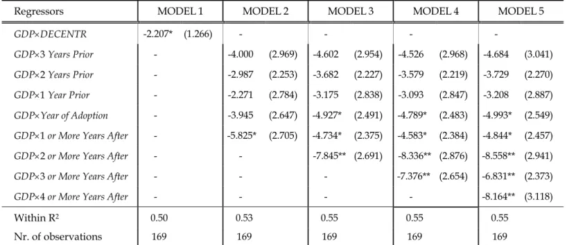
Table 5. The impact of fiscal decentralization on health inequalities excluding Regions with a high deficit in the post-reform period (a)
(a) The excluded Regions (Lazio and Campania) are those whose deficits for health spending in the period 1998-2007 summed up to more than 50% of the whole aggregated deficit computed for all Regions. The dependent variable is the index of inequality in self-assessed health (KM). Cluster–robust standard errors at the Region level are reported in round brackets. All models include the vector of control X, regional and year FE. MODEL 2-5 extend the baseline specification to include leads (GDP×1 Year Prior = 1997,
GDP×2 Years Prior = 1996, GDP×3 Years Prior = 1995) and lags (GDP×1 or More Years After refers to time period 1999-2007 in MODEL 2
and only to year 1999 in MODELS 3-5; GDP×2 or More Years After refers to time period 2000-2007 in MODEL 3 and only to year 2000 in MODELS 4-5; GDP×3 or More Years After refers to time period 2001-2007 in MODEL 4 and only to year 2001 in MODEL5; GDP×4 or
More Years After refers to time period 2002-2007). GDP×Year of Adoption refers only to the effect of decentralization observed in year
1998.
**statistically significant at 5%; *statistically significant at 10%.
Secondly, we consider the issue of regional deficits by considering a reduced sample which excludes Lazio and Campania, the two regions whose deficits for health spending in the period 1998-2007 (after the reform was implemented) summed up to more than 50% of the whole aggregated deficit for healthcare in Italy (Tediosi et al., 2009). Table 5 shows the estimates of Equation [1] on this reduced sample. Our initial results are confirmed again: the tax reform caused a containment of within-regional health inequalities more pronounced in rich regions compared to poor ones; moreover, the magnitude of the impact
increases over time and is almost double after two years of the introduction on the new regional taxes.
Regressors MODEL1 MODEL2 MODEL3 MODEL4 MODEL5
GDP×DECENTR -2.308** (0.908) - - - -
GDP×3 Years Prior - -3.055 (2.824) -3.647 (2.826) -3.545 (2.852) -3.752 (2.967)
GDP×2 Years Prior - -2.273 (1.951) -3.011 (1.933) -2.866 (1.945) -3.098 (2.075)
GDP×1 Year Prior - -2.429 (2.652) -3.348 (2.632) -3.216 (2.664) -3.448 (2.809)
GDP×Year of Adoption - -3.682 (2.327) -4.773* (2.249) -4.576* (2.281) -4.922* (2.452)
GDP×1 or More Years After - -5.469** (2.549) -4.325* (2.296) -4.112* (2.354) -4.529* (2.541)
GDP×2 or More Years After - - -7.702*** (2.563) -8.031*** (2.641) -8.474** (2.872)
GDP×3 or More Years After - - - -7.164** (2.650) -6.936** (2.444)
GDP×4 or More Years After - - - - -8.041** (3.244)
Within R2 0.48 0.50 0.52 0.53 0.53
Nr. Of observations 195 195 195 195 195
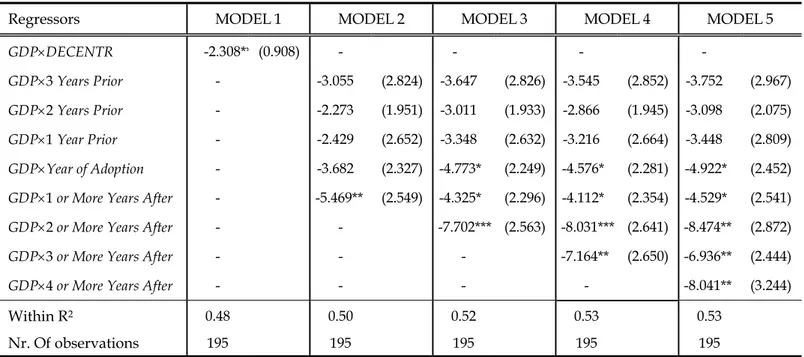
Table 6. The impact of fiscal decentralization on health inequalities controlling also for the effect of the quasi-markets reform (a)
(a) The effect of the quasi-markets reform is tested by including in the vector of controls X also a dummy variable QM equal to one when the Regions adopt their own set of DRG tariffs. The dependent variable is the index of inequality in self-assessed health (KM). Cluster–robust standard errors at the Region level are reported in round brackets. All models include the vector of control X, regional and year FE. MODEL 2-5 extend the baseline specification to include leads (GDP×1 Year Prior = 1997, GDP×2 Years Prior = 1996, GDP×3
Years Prior = 1995) and lags (GDP×1 or More Years After refers to time period 1999-2007 in MODEL 2 and only to year 1999 in MODELS
3-5; GDP×2 or More Years After refers to time period 2000-2007 in MODEL 3 and only to year 2000 in MODELS 4-5; GDP×3 or More
Years After refers to time period 2001-2007 in MODEL 4 and only to year 2001 in MODEL5; GDP×4 or More Years After refers to time
period 2002-2007). GDP×Year of Adoption refers only to the effect of decentralization observed in year 1998. **statistically significant at 5%; *statistically significant at 10%.
We next consider the potential source of bias stemming from the quasi-market reform implemented in Italy during the Nineties. This reform, inspired by the UK experience, was aimed at improving spending efficiency (the same goal of the tax decentralization reform) working at a more micro level. In particular, it was hoped that the introduction of a new prospective payment scheme for hospitals with fixed prices based on Diagnosis Related Groups, would increase spending efficiency. The new payment system became effective in 1997, and regions were allowed to differentiate tariffs with respect to national prices. However, few regions introduced their own tariffs and those that did, did so at different times: in particular, some of the richest regions (Lombardy and Emilia Romagna) were among the first to adopt their own set of tariffs beginning in 1997, followed by Veneto in 1998. We exploit this variability across regions and years in the adoption of own tariffs to define the dummy variable QM, (quasi-markets), taking value one when a region adopted a
set of tariffs different from the national ones. Table 6 presents the estimates obtained from an augmented version of Eq. [1], which also includes the variable QM among the covariates. Our results are largely confirmed in this case, in terms of sign, magnitude and significance. Moreover, the coefficient of the variable QM is never statistically significant at the usual confidence levels, suggesting that the introduction of quasi-markets did not have any impact on inequalities. This finding is in line with Cappellari et al. (2016), who show that price incentives introduced by the quasi-markets reform did not affect perceived health. The authors argue that the quasi-market reform reduced inappropriate access to some services, with stronger effects in the first years immediately after the reform in regions that adopted their own set of tariffs.
Regressors MODEL1 MODEL2 MODEL3 MODEL4 MODEL5
GDP×DECENTR -1.878** (0.790) - - - -
GDP× 3 Years Prior - -1.641 (1.966) -2.086 (1.990) -2.037 (2.001) -2.063 (2.072)
GDP× 2 Years Prior - -1.750 (1.608) -2.349 (1.745) -2.280 (1.778) -2.317 (1.888)
GDP×1 Year Prior - -0.454 (1.935) -1.192 (2.016) -1.114 (2.029) -1.146 (2.139)
GDP×Year of Adoption - -2.105 (1.801) -2.954 (1.934) -2.861 (1.966) -2.906 (2.095)
GDP×1 or More Years After - -3.345* (1.918) -2.314 (1.738) -2.220 (1.763) -2.278 (1.930)
GDP× 2 or More Years After - - -5.082** (2.246) -5.268** (2.224) -5.332** (2.408)
GDP× 3 or More Years After - - - -4.820* (2.345) -4.740** (2.138)
GDP× 4 or More Years After - - - - -4.957* (2.810)
Within R2 0.50 0.51 0.52 0.53 0.53
Nr. of observations 247 247 247 247 247
Table 7. The impact of fiscal decentralization on health inequalities considering also Special Status Regions in the sample (a)
(a) The dependent variable is the index of inequality in self-assessed health (KM). Cluster–robust standard errors at the Region level are reported in round brackets. All models include the vector of control X, regional and year FE. MODEL 2-5 extend the baseline specification to include leads (GDP×1 Year Prior = 1997, GDP×2 Years Prior = 1996, GDP×3 Years Prior = 1995) and lags (GDP×1 or More
Years After refers to time period 1999-2007 in MODEL 2 and only to year 1999 in MODELS 3-5; GDP×2 or More Years After refers to
time period 2000-2007 in MODEL 3 and only to year 2000 in MODELS 4-5; GDP×3 or More Years After refers to time period 2001-2007 in MODEL 4 and only to year 2001 in MODEL5; GDP×4 or More Years After refers to time period 2002-2007). GDP×Year of Adoption refers only to the effect of decentralization observed in year 1998.
**statistically significant at 5%; *statistically significant at 10%.
Finally, Table 7 reports the estimates of Eq. [1] on a larger sample which also includes the Special Statute Regions (Friuli Venezia Giulia and Trentino Alto Adige in the North, Sardinia and Sicily in the South). These regions differ markedly in terms of population and GDP per-capita, but most of all in terms of the specific fiscal relationships they maintain
with the central government.20 Although the main conclusions of our study are still valid,
all coefficients of interest are now lower in magnitude than those obtained in Table 3. This is consistent with the fact that Special Statute Regions are largely unaffected by the fiscal decentralization reform, and thus their inclusion in the sample is expected to dilute the estimated average treatment effect.
5.3. Discussion
In this section we discuss some of the potential mechanisms that can explain why tax decentralization helped contain within-regional inequalities in health outcomes more in rich regions than in poor ones. The modern theories of fiscal decentralization suggest a story of
incentives: local officials that need to raise more resources via own revenue are more
accountable to their citizens. In turn, more accountable politicians might provide market-enhancing public goods, which positively influence economic growth at the local level; or they might offer better and more easy-to-access health care services; or they might supply more appropriate and more targeted services because of better governance. We explore each of these explanations in turn.
A first possible mechanism underlying the relationship between increased accountability of regional governments and the ability to contain health disparities may be related to regional economic growth (e.g., Akai and Sakata, 2002; Weingast, 2009). A higher degree of fiscal autonomy might have stimulated growth at the local level. A higher income, in turn, might have affected private health spending. We follow two strategies to investigate formally the validity of this argument. Firstly, we test the impact of decentralization on both per capita GDP and private health spending by estimating a model mirroring Equation [1] with a complete set of leads and lags of the treatment, where the effect of the tax reform is allowed to be different in rich and poor regions (used as the treated and control groups, respectively). In particular, we define the dummy variable RICH to identify regions with per-capita income above the sample mean, and interact this variable with DECENTR, the indicator of the post-decentralization period. As expected, for both variables we found a large difference in the trend of growth between the two groups of regions, but no evidence of any divergence caused by decentralization: per capita GDP and private health spending grew more in the North than in the South over the entire 1994-2007 period (Appendix Table
20 For instance, the two autonomous provinces making up Trentino Alto Adige retain almost all the revenues
they raise in their territory, receiving virtually no transfers from the central government, and also having spending autonomy on education. On the contrary, Sicily receives transfers from the central government even if it retains revenues and does not have spending autonomy on education.
A.2). To confirm this finding, we also re-estimated our original models in Table 3 by substituting per capita public spending with per capita total spending for health care. Baseline results are generally unaffected when considering total spending instead of public spending (Appendix Table A.4). These results provide no evidence to support the hypothesis that the differential effect of fiscal decentralization is driven by an “income” effect.
A second possible mechanism is patient migration. Suppose that – following the reform – increased accountability induced local politicians in the richest regions to provide even better services, increasing the differential in terms of quality with respect to poor regions21.
Patient-inflow from poor regions would then have increased, exacerbating disparities in the
Mezzogiorno among patients able to migrate to other regions (likely the richer) and those
who are not (the poorer). Brekke et al. (2016) provide a similar argument in a model where regions are fully responsible for financing their healthcare systems and spending is completely funded with local resources. In particular, the authors show that, if inter-regional inequality increases, then we will observe an increase in the quality of services in high-income regions and an opposite effect in low income regions. Under this hypothesis, the effect in the high-income region is driven by the increase in income: quality improvements will be financed by the increase in local taxation, since the marginal cost of taxation is now lower. The improved quality will then trigger an increase in patient mobility from low-income regions. Parallel effects will be observed if intra-regional inequality in income increases.
As already observed, income inequality across regions does not play a direct role in the case of the Italian NHS, since a system of equalization grants to supply the same set of quasi-universal services is in place. In the presence of equalization grants, an increase in inter-regional inequality will increase the reliance of rich-regions on their own resources, and poor regions will receive additional transfers from the center. Moreover, rich regions did not seem to have exploited fiscal autonomy given the mandatory quasi-universal set of services to be provided in all regions. However, we investigate formally the validity of patient migration as a potential explanation of our findings by considering the compensation mechanism in place in Italy to account for the free choice of patients. Suppose that a patient migrates from Region i in the South to Region j in the North. If this occurs, Region i must compensate Region j for the treatment provided to the patient paying a tariff
defined at the national level. We consider total net compensations received by each region in a model including a full set of leads and lags, allowing the impact of the tax reform to be different in rich and poor regions (categorised as the treated and control groups, respectively) again using the dummy RICH. The relevant coefficients are insignificant, suggesting that patients’ migration cannot explain our findings (Appendix Table A.2). This argument is further supported by an additional model designed to check whether the perceived quality of health services changed differently after the tax reform in rich and poor regions (Appendix Table A.3). If the quality differential has widened, then inequality might have increased even without any changes in the outflow of patients. However, there is no evidence of any significant differential changes in patient satisfaction for medical and nursing care, nor for the cleanliness of hospital toilets that could justify the increase in inequality in the absence of any changes in migration flows from poor to rich regions.
Finally, a third explanation is based on the idea that more accountable politicians will supply more appropriate and more targeted services, improving the governance of the regional healthcare system. In this respect, regional screening programs for cancer prevention – in particular, the malignant tumors affecting breast, colon and uterus – represent an interesting policy issue to consider. For instance, breast cancer is one of the most important concerns for health in Europe because of its high incidence and mortality (e.g., Ferlay et al., 2013). Moreover, recent empirical evidence highlights that inequalities in the use of mammography are stronger in countries like Italy that does not have a national screening program; and the effectiveness of these programs in increasing preventive use is higher among the women with lower education (e.g., Carrieri and Wuebker, 2016). In general, this suggests that if – following fiscal decentralization – rich regions were more able to introduce effective screening programs, we expect to observe a higher increase of cancer prevention rates and citizens’ health in these regions; and the difference with respect to poor regions should be particularly marked for less educated people. As those less educated are presumably also poorer individuals, unlikely to turn to private providers to purchase out-of-pocket screening tests, this might help explain why in Southern regions we observe a deterioration of health inequalities relative to Northern ones.
Unfortunately, we cannot directly test the effects of fiscal decentralization on cancer prevention rates, as we do not have yearly information on the adherence to screening programs in the period before and after the tax reform for individuals with different education levels. However, individual-level data from the 1994–2007 Multiscopo ISTAT


![Table 2. Summary statistics of the variables used in model [1]](https://thumb-eu.123doks.com/thumbv2/123dokorg/8339941.132923/18.892.117.775.111.586/table-summary-statistics-variables-used-model.webp)