A problem in demand aggregation : per capita demand as a function of per capita expenditure

(1)

©

The

Author(s).

European

University

Institute.

by

the

EUI

Library

in

2020.

Available

Open

Access

on

Cadmus,

European

University

Institute

Research

Repository.

(2)

©

The

Author(s).

European

University

Institute.

version

produced

by

the

EUI

Library

in

2020.

Available

Open

Access

on

Cadmus,

European

University

Institute

Research

Repository.

(3)

A PROBLEM IN DEMAND AGGREGATION:

PER CAPITA DEMAND AS A FUNCTION OF PER CAPITA EXPENDITURE Werner Hildenbrand

1. Introduction

The expenditure elasticity for a certain commodity is a well defined concept if it refers to a single individual. Yet this case is irrelevant and the concept is never used in such a situation. In all applications the concept of expenditure elasticity refers to a population (a group of individuals): one wants to know how per capita demand for a certain commodity o f a given population changes if per capita expenditure of that population varies.

We take it as a fact that ’’ people are different” ; different in tastes (preferences), income and other characteristics (attributes). In this context the concept of expenditure elasticity is relevant and used. Yet how the concept is defined in this case?

Obviously, what is needed is a functional relationship between per capita demand and per

capita expenditure, ceteris paribus, i.e. a ” macro” -demand function.

Consequently, either one assumes the existence of such a relationship right away, than the problem is ’’ solved” by assumption. Or one has to specify a micro-economic model of a population (group of households), which allows ’’ people to be different” , such that the impact of a change in per capita expenditure is well determined.

In this note we shall discuss the conceptual difficulties for the existence of a macro-demand function, i.e., a functional relationship between per capita demand, prices of all commodities and per capita expenditure. We shall also discuss the question under which conditions on the underlying micro-model one can estimate the expenditure elasticities from cross-section data.

In section 2 we shall first define the market demand function and then in section 3, we shall discuss the aggregation problem.

©

The

Author(s).

European

University

Institute.

by

the

EUI

Library

in

2020.

Available

Open

Access

on

Cadmus,

European

University

Institute

Research

Repository.

(4)

2. Mean demand

The basic primitive concept of traditional demand theory is the individual demand function; it is assumed that for every individual household there is a functional relationship / between his expenditure (budget, total outlay) b, the prevailing price system p and his demand i for the various commodities.

x = f(p ,b ) <E Rl+ , P € f ? + , b > 0.

This functional relationship / is thought to be determined by individual characteristics of the household which are relevant in the consumption decision. Some of these consumption charac teristics are directly observable others are not.

In neoclassical demand theory all individual consumption characteristics are summarized by the concept of an individual preference relation ■< (or utility function). Given an individual preference relation ■<, then the ’’ hypothesis of preference maximization” determines the indi vidual demand function / ( - , - , ;<). O f course these demand functions / ( - ,- , ;<) will have certain general properties reflecting the fact that they are obtained as the result of a maximization problem. Thus, the “hypothesis of preference maximization” is a general and elegant way to

parametrize a certain class / ( - , - , :<) o f individual demand functions, the parameter being the

preference relation. Since we have no reasonable criterion to decide which preference relation describes plausible consumption behaviour1) the class of individual demand functions defined in this way is very large.

Let P denote the set of all preference relations on R + , which lead to continuously differen tiable demand functions f(p , •, ■<) with respect to b.

For the purpose of demand analysis an individual household t is completely characterized by his expenditure b' and his preference relation ^*, i.e., by a point (6*, ;<*) in the cartesian product R+ x P.

x) The choice of a particular preference relation < is typically justified by the plausibility of the demand function /(•, -, ;<) which is derived from it.

2

©

The

Author(s).

European

University

Institute.

version

produced

by

the

EUI

Library

in

2020.

Available

Open

Access

on

Cadmus,

European

University

Institute

Research

Repository.

(5)

A group G o f households is then represented by a “cloud” {(6*, r^‘ )}ie G o f points in R+ x P .

Figure 1

Since we are mainly interested in large groups G of households we shall describe the “cloud” of points in R+ x P by its (empirical) joint distribution p c , i.e.,

Pa( B) =

e

G

I

(b\ 1*)

ell},

B C R+

x

p.

WG

With this notation we have the identity

£ /( p , &*, =

f

/( p , *>,

#:Cr ^

J

r

+

x

P

Definition: The mean (per capita) demand (or market demand) o f a group o f households (which

is described by the joint distribution p o f expenditure and preferences) is defined by

B(p,p)’-=

f

f(p,b,<)dp

J

r

+

xp

This definition of mean demand can be extended to more general distributions p than the em pirical distributions of finite groups o f households. This will be done in the sequel, in particular, we shall consider distributions p where the corresponding marginal distributions of expenditures

©

The

Author(s).

European

University

Institute.

by

the

EUI

Library

in

2020.

Available

Open

Access

on

Cadmus,

European

University

Institute

Research

Repository.

(6)

axe given by densities, like the log normal distribution. If the space P of preferences is endowed with a metric (see e.g. Hildenbrand 1974) then we can extend the above definition of mean de mand to any (Borel) probability distribution on the cartesian product R.y x P . We shall always assume that the mean of the expenditure distribution is finite.

Remark

In applied demand analysis and in some econometric models (e.g. D. W. Jorgensen, L.J. Lau and T.M. Stoker 1982) one often uses a more specific version of this model. One starts with a list a j, a2 ■. ., a „ of observable consumption characteristics, called attributes (e.g., families* total

expenditures, family size, age (sex) composition of the families,...) and postulates a functional relationship between the price system p, the attributes a = (a 1,0,2 . . . an) and the demand vector

x e Rl ,

x = g(p,a), p e R l+ , a & A.

The group of households (population) is then described by a distribution a of attributes. Thus, mean demand is defined by

F(P, a ) = / g{p, a)da. J A

To link this model to our preference based formulation, we start from the hypothesis that individual preference relations are dependent on attributes, < a ■ There is no list of observable

attributes - as detailed and long this list might be - such that households with the same

attributes a = (a 1, «2 . . . ) have identical demand behavior. Thus, there is a gap between prices of all commodities, observable attributes and demand. Indeed, individual preference relations (utilities) have been invented to fill this gap. Consequently, g(p, a) is not in a strict sense an individual micro demand relationship. It has to be interpreted as an average, the mean demand of all those households in the group with attributes a (households of type a.) Thus, in the notation of our model, where the group of households is described by a joint distribution p of expenditures and preferences we define

9{P, «) = j ' /(P, b, <)dp | o,

where p | a denotes the conditional distribution of preferences given the attribute a = («1 — bi,d2, ■ ■ •)

Thus

F{P, P) =

J

f{p,b, <)dp = f A( f p f ( P' b> —)dp I a)da = g(p,a)da.

The usefulness of the “attribute-model” (A, g, a) rests on the hypothesis that the demand re

lation g(p,a) for types o f households is relatively stable for variations of the distribution p, in

particular, if the distribution p changes over time.Thus, if the distribution p changes and if the function g(p, a) does not change (e.g. if the conditional distributions p | a do not change)

4

©

The

Author(s).

European

University

Institute.

version

produced

by

the

EUI

Library

in

2020.

Available

Open

Access

on

Cadmus,

European

University

Institute

Research

Repository.

(7)

then the change o f the distribution p, can he attributed solely to a change of the observable distribution a on the space A of attributes.

The advantage or disadvantage of these two models are obvious. The advantage of the attribute-model is that the distribution a, and hence its evolution over time, can, in principle, be observed since by definition the attributes are observable. The disadvantage of this model (from a theoretical point of view!) is that it is not clear which general properties of the function g(p, a) one can postulate, since g(p, a) is the mean demand of ail households of type a. For example, the axiom of revealed preferences does not necessarily hold. In other words, the attribute-model assumes that the aggregation problem for households of the same type is settled. On the other hand, in the preference-model the individual demand functions are canonically defined (through • ;<), and the general properties of the functions / ( - ,- , :<) are well known. The disadvantage, of

course, is the fact, that the full distribution p is not observable.

In the literature the function g(p, a) is often interpreted as an individual demand relation by adding a random term

g(p, a) + £„

where ea represents a random vector with expectation E( ea) = 0, wliich is supposed to take into account the different consumption behavior within the type a. Thus, ea is a random vector on the probability space

( P, p | a); £„(;<) = [ f{p,b, <)dp \ a - f ( p , b ;<).

Jp •

In this generality there is no substantial difference between the attribute-model f A g(p, a)da and the preference-model f R+xp f{p,b, ^)dp. Yet, the two models differ substantially as soon as one specifies the functional form of g (e.g. linear in a A C Rn) and the stochstic structure of the random terms £„ (e.g. independence or homoscedasticity.) The following discussion applies to both models. 5

©

The

Author(s).

European

University

Institute.

by

the

EUI

Library

in

2020.

Available

Open

Access

on

Cadmus,

European

University

Institute

Research

Repository.

(8)

3.1. The motivation for considering mean demand as a function of mean expenditure comes mainly from applied demand analysis. If one wants to estimate a demand system the above definition of market demand as

P ( p , p ) - f f(p,f>,^)dp

Jr+xP

is much too detailed. The full distribution p of agents1 characteristics on 1?+ X P can, of course, not be observed.

In these applications F(p, p) is often interpreted as a short run demand system2! i.e., all commodities refer to a certain period t. Thus, let p t describe the distribution of agents1 characteristics in period t and consider a time series (pt), t — 1 , . . . , T of joint distributions of agents1 characteristics. Let B t denote the mean expenditure associated with the distribution p t. Problem 1: Under which condition on the evolution (pt), does there exist a function C(p, B),

the “macro” demand function, such that

F ( p , p t) — C ( p , B t) for every t and p ?

Remark: The question is not restricted to the interpretation of t as “time” . One might consider a subset D (not just a one-parameter path) of distributions on R+ X P and ask whether F(p, p) =

C (p, B) for every p € D and p.

3. Mean (per capita) demand as a function of mean (per capita) expenditure

In most empirical demand studies (see e.g. the survey paper by Brown and Deaton (1972) in The Economic Journal) market demand is written in the simplified form C(p, B ). One then typically is interested in

]ffjCh(P) B), the marginal propensity to consume (M P C ) commodity h out of per capita

expenditure B or

Ci^WjWBC h(p,B), the expenditure elasticity (EE) for the group p of commodity h.

Problem 2: Given a solution to Problem 1, under which condition on the evolation (pt) is it possible to estimate the M P C or E E from cross-section data of family expendi tures?

21 This interpretation strictly speaking requires an intertemporal setting (for an analysis of short-run demand functions, see e.g., Grandmont (1982)). We neglect the intertemporal aspect jn order to simplify the presentation. The present analysis has to be extended if it were applied to a situation where the intertemporal aspect cannot be neglected, for example, in the theory of consumption functions. 6

©

The

Author(s).

European

University

Institute.

version

produced

by

the

EUI

Library

in

2020.

Available

Open

Access

on

Cadmus,

European

University

Institute

Research

Repository.

(9)

The distribution p t cannot be observed. In principle, one can observe the expenditure and demand vector for every individual i in the group G :

( b l r t (Pt,b\))ieG

Let ut denote the joint distribution of expenditure and demand, i.e., vt is the image measure of

fit under the mapping

(6, < ) ^ ( b , f ( P, b ± ) ) .

Figure 2

We assume that cross-section data of family expenditures give us, in principal, a sample distribution of vt\ If the distribution vt is known one can compute

1) the empirical distribution function o f expenditure Vt

Vt(o - Pt({b, < ) e R + x P \ b < £ } ) = **({(6 ,*) € fl‘++1 I b < 0 ) and

©

The

Author(s).

European

University

Institute.

by

the

EUI

Library

in

2020.

Available

Open

Access

on

Cadmus,

European

University

Institute

Research

Repository.

(10)

C M =

I

h ( p , b , < )d pt

I

b

=

E {vt

I

b)h

where pt | b (reap. vt | 6) denotes the conditional distribution o f p t (resp. i^t) given b, i.e., pt | b (resp. i/t | 6) denotes the distribution of preferences (resp. demand vectors) of those households whose expenditure is equal to b. If it is clear from the context which distribution p is used then I shall Write / instead of / M.

In the following I shall neglect the statistical aspect of the problem. That is to say, the cross-section data of family expenditures at time t give us at best a sample distribution of

i/t . Hence every number which is derived from cross-section data is a random variable. I do

not study in this paper the statistical properties of such random variables. I shall, however, assume in the following that the distributions are known. I think that this is a characteristic difference between economic theory and econometrics. The theorist uses full information, i.e., the distribution vt , while the econometrician explicitly takes into account that one can only observe a sample distribution of vt . To carry out then the statistical analysis one has, unfortunately, often to make strong and unjustifiable assumptions on the distribution p, in particular, on its support.3) For a theoretical analysis some of these assumptions are not necessary.

There would be a trivial solution to Problem 1 and 2 if one could assume that the Engel curves for every commodity h were

(i) linear in b and

(ii) independent o f t, at least at the relevant domain of the expenditure distribution, i.e.,

C M = / ( P,6).

2) the Engel curve o f the group for every com m odity h, i.e.,

3) For an econometric approach to the problem of aggregation which is in the line of this note we refer to the work of T.M.Stoker, in particular to ’’ Completeness, Distribution Restrictions, and the Form of Aggregate Functions” , Econometrica 1985.

8

©

The

Author(s).

European

University

Institute.

version

produced

by

the

EUI

Library

in

2020.

Available

Open

Access

on

Cadmus,

European

University

Institute

Research

Repository.

(11)

h

Figure 3

Indeed, in this case one obtains

F(P, Mt) = f /(P , b)dVt(b) = /( p , B t). JR+

The textbook example (e.g., Deaton and Muellbauer (1980) Chapter 6 or the surveÿ paper by Shafer and Sonnenschein (1982)) for such a case is the situation where all households have * the same homothetic preference relation.4^ Note that homothetic, but not identical preferences do not imply that the Engel curve /( p , •) is linear, nor does linearity of /( p , -) imply that the individual demand functions /( p , 6, ■<) are linear in b.

In any case cross-section studies of family expenditures indicate clearly that Engel curves /( p , •) for specific commodities are typically not linear, even if restricted to the relevant domain of the expenditure distribution. Even for very broad commodity aggregates is this assumption not well supported by empirical evidence.

4) In this case /( p , •) is even homogeneous of degree one, thus one has E E — 1, hence there is nothing to be estimated. The empirical analysis is needed only to check the hypothesis of the linearity of the Engel curve /( p , •).

9

©

The

Author(s).

European

University

Institute.

by

the

EUI

Library

in

2020.

Available

Open

Access

on

Cadmus,

European

University

Institute

Research

Repository.

(12)

If we take it for granted that typically Engel curves /( p , ■) are not linear then mean de mand depends on the distribution of expenditures.5) This fact, of course, is well-known and is emphasized in the literature. Some economists build their theory on this fact; for example, Keynes, if he proposes measures of redistribution of income with the aim of stimulating market demand. However, in the econometric models the distributional effect is often neglected. The importance of the distributional aspect is very clearly discussed by J. Marschak in several papers in the 1930s (Econometrica (1939) and Review o f Economic Statistics (1939)), by T. Haavelmo,

(Econometrica (1947)) and by P. de Wolff (Economic Journal (1941)). They also discuss the

use of cross-section data and come to quite different conclusions. As we shall see the reason for this apparent contradiction is that they make quite different assumptions on the evolution of

(fit)- For a more recent reference we refer to the excellent discussion of the aggregation problem

in E. Malinvaud, Théorie M acroéconom ique (1981) Chapter 2.2.

Problem 1, but not necessarily Problem 2, has again an obvious solution (a “solution” by assumption) if we restrict the evolution (pt) to a one-parameter family, where the parameter can be chosen to be the mean B t o f the expenditure distribution in period t. There are, of course, alternative ways to specify such parametrization of the evolution (pt)- Different specifications will lead to different macro-demand functions C(p, B).

5) There is a well known exceptional case, studied by Gorman (1953) and Nataf (1953), where the statistical Engel curves of the group might not be linear and still mean demand depends only on mean expenditures. Indeed, if preferences are such that for every commodity h the

individual demand function /( p , b, X) is on the relevant domain of the expenditure distribution, linear in b and has for all households the same slope S^, then

Fh(p,p) — [ ( f h ( p , B , < ) - (B - b ) S h) d p = f f h( p , B , < ) d p ^ ,

JR+X.P

J

p

where p_< denotes the marginal distribution of preferences of the distribution fi. Thus, if in addition to the strong assumptions on the indivudual demand functions the marginal distribution of preferences is fixed, then meand demand depends only on mean expenditure. This, however, is too special a case to be considered as a solution to problem 1.

10

©

The

Author(s).

European

University

Institute.

version

produced

by

the

EUI

Library

in

2020.

Available

Open

Access

on

Cadmus,

European

University

Institute

Research

Repository.

(13)

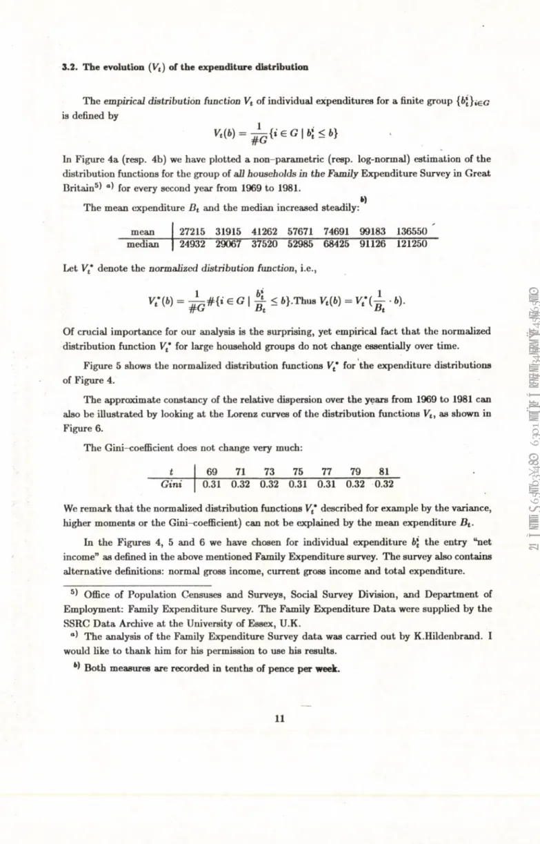
3.2. The evolution (Vt) of the expenditure distribution

The empirical distribution function Vt of individual expenditures for a finite group {6J},£g

is defined by

Vt(b) = ~ { i 6 G i 6* < 6}

In Figure 4a (resp. 4b) we have plotted a non-parametric (resp. log-normal) estimation of the distribution functions for the group of all households in the Family Expenditure Survey in Great Britain5^ °) for every second year from 1969 to 1981.

„ *) The mean expenditure Dt and the median increased steadily:

mean 27215 31915 41262 57671 74691 99183 136550 ' median 24932 29067 37520 52985 68425 91126 121250 Let V" denote the normalized distribution function, i.e.,

K W = ^ # { * ‘ € G I ^ < 6 }.Thus Vt(b) = • b).

Of crucial importance for our analysis is the surprising, yet empirical fact that the normalized distribution function Ft* for large household groups do not change essentially over time.

Figure 5 shows the normalized distribution functions Vt* for the expenditure distributions of Figure 4.

The approximate constancy of the relative dispersion over the years from 1969 to 1981 can also be illustrated by looking at the Lorenz curves of the distribution functions Vt, as shown in Figure 6.

The Gini-coefficient does not change very much:

t 69 71 73 75 77 79 81

Gini 0.31 0.32 0.32 0.31 0.31 0.32 0.32

We remark that the normalized distribution functions Vt* described for example by the variance, higher moments or the Ginicoefficient) can not be explained by the mean expenditure Dt

-In the Figures 4, 5 and 6 we have chosen for individual expenditure b\ the entry “net income” as defined in the above mentioned Family Expenditure survey. The survey also contains alternative definitions: normal gross income, current gross income and total expenditure.

5) Office o f Population Censuses and Surveys, Social Survey Division, and Department of Employment: Family Expenditure Survey. The Family Expenditure Data were supplied by the SSRC Data Archive at the University of Essex, U.K.

“ ) The analysis of the Family Expenditure Survey data was carried out by K.Hildenbrand. I would like to thank him for his permission to use his results.

k) Both measures are recorded in tenths of pence per week.

©

The

Author(s).

European

University

Institute.

by

the

EUI

Library

in

2020.

Available

Open

Access

on

Cadmus,

European

University

Institute

Research

Repository.

(14)

s o -b o s - e SQ -309'1 7 5 0 0 0 1 5 0 0 0 0 2 2 5 0 0 0 3 0 0 0 0 0 F ig u re 4a: N o n -p a r a m e tr ic e s ti m a ti o n o f th e d is tr ib u ti o n f u n c ti o n s o f e x p e n d it u r e s f o r a ll h o u s e h o ld s (1 9 6 9 , 1971, 1973, 1975, 1977, 19 79, 198 1) ( “D is c r e te M a x im u m P e n a liz e d L ik e li h o o d E s ti m a ti o n ” )

©

The

Author(s).

European

University

Institute.

version

produced

by

the

EUI

Library

in

2020.

Available

Open

Access

on

Cadmus,

European

University

Institute

Research

Repository.

(15)

i r 5 0 -3 0 5 'G o f F ig » * *

©

The

Author(s).

European

University

Institute.

by

the

EUI

Library

in

2020.

Available

Open

Access

on

Cadmus,

European

University

Institute

Research

Repository.

(16)

ocri

os’o

F ig u re 5: N o rm a li z e d d is tr ib u ti o n f u n c ti o n s f o r t h e g r o u p o f al l h o u s e h o ld s

©

The

Author(s).

European

University

Institute.

version

produced

by

the

EUI

Library

in

2020.

Available

Open

Access

on

Cadmus,

European

University

Institute

Research

Repository.

(17)

D

C

•

15

Figure 6: Lorenz curves of the distribution functions Vt

©

The

Author(s).

European

University

Institute.

by

the

EUI

Library

in

2020.

Available

Open

Access

on

Cadmus,

European

University

Institute

Research

Repository.

(18)

In all cases one obtains essentially the same pictures. Figures 7 and 8 illustrate the distribution for the entry “total expenditure” .

This approximate constancy over time of the normalized expenditure distributions is, of course, well known in the literature on personal income distributions.6^ The foregoing discussion motivates the following

Assumption 1: (the law o f constant relative dispersion)

The normalized distribution functions Vt° do not change along the evolution (/it)- Thus, there is a distribution function V ' with mean equal to one such that

Vt(6) = V * ( i - - 6 )

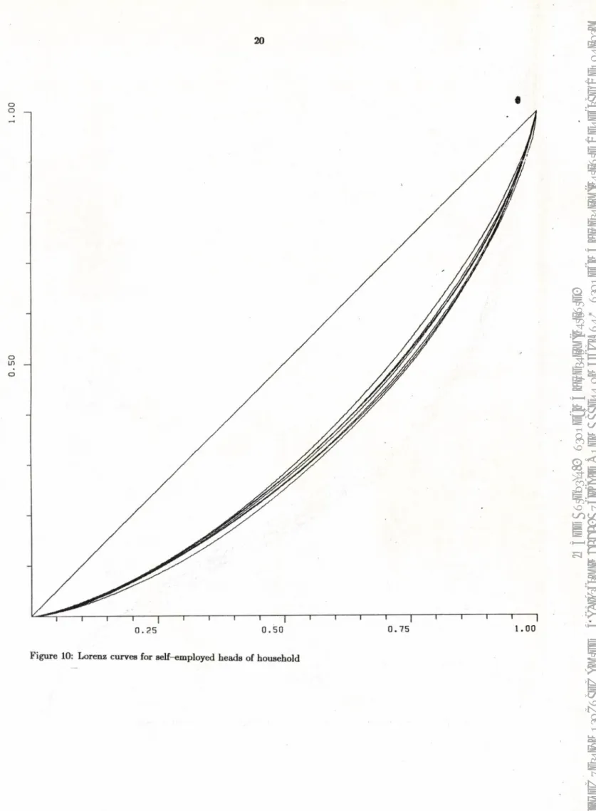
This is, indeed, a strong assumption on the evolution of the distributions of expenditures. It implies that the Gini coefficient and the Lorenz curve of the expenditure distributions Vt do not depend on t. However, as we have shown, the assumption is surprisingly well supported by empirical studies provided it is applied to the group of all households in a country. It is known that the law of constant relative dispersion does hold less well for subgroups, like self-employed heads of household or retired individuals (see Figures 9 and 10).

If one considers the remaining differences in the normalized distribution functions Vt* (see e.g. Figure 5) as still relevant, then in the macro-demand function one has to take into account in addition to the mean B t other characteristics of the distribution Vt as well. Note, however, we

c i r é not interested here in the distributions Vt per se;we do not discuss econdenz inequality. The

relevant question is whether the remaining differences in the normalized distribution functions

Vt* have a relevant influence on mean demand, i.e., on the integral

I f(p,b)dVt(b) = I f ( p , B t - b ) d V ; ( b ) ~ I f ( p , B t b)dV'(b).

At this point I will not pursue a discussion and justification of the “law of constant relative dispersion” . For the time being I take it as an example for a simple assumption which leads to a one-parameter family of distribution functions Vt, where the mean B t each distribution can

be chosen as the parameter.

6) e.g. G. Vangrevelinghe, “Les niveaux de vie en France —1956 et 1966” . Economie et

Statistique N o.l 1969, G. Banderier “Repartition et evolution des revenus fiscaux des ménage” Economie et Statistique No. 16, 1970 and G. Goseke and K.D. Bedau (1974), Verteilung und

Schichtung der Einkommen der privaten Haushalte in der BRD von 1950-1975. Deutsches Institut fiir Wirtschaftsforschung, Heft 31, (Duncker und Humblot, Berlin), A.S. Blinder, “The level and distribution of Income Well Being” , in: The American Economy in 'JYansition (ed. M. Feldstein), Univ. of Chicago Press 1980, J. Hartog and J.G. Venbergen, Dutch treat, long run changes in personal income distribution, De Economist 126, Nr.4, 1978

16

©

The

Author(s).

European

University

Institute.

version

produced

by

the

EUI

Library

in

2020.

Available

Open

Access

on

Cadmus,

European

University

Institute

Research

Repository.

(19)

ro « 7 : D is tr ib u ti o n f u n c ti o n s f o r “T o ta l E x p e n d i t u ri

©

The

Author(s).

European

University

Institute.

by

the

EUI

Library

in

2020.

Available

Open

Access

on

Cadmus,

European

University

Institute

Research

Repository.

(20)

18

a

Figure 8: Lorenz curves for “Total Expenditure”

©

The

Author(s).

European

University

Institute.

version

produced

by

the

EUI

Library

in

2020.

Available

Open

Access

on

Cadmus,

European

University

Institute

Research

Repository.

(21)

u r e 9: D is tr ib u ti o n f u n c ti o n s o f ‘n e t in c o m e ’ fo r s e lf -e m p lo y e d h e a d s o f h o u s e h o ld

©

The

Author(s).

European

University

Institute.

by

the

EUI

Library

in

2020.

Available

Open

Access

on

Cadmus,

European

University

Institute

Research

Repository.

(22)

.5 0 1 .0 0 20

«

Figure 10: Lorenz curves for self-employed heads of household

©

The

Author(s).

European

University

Institute.

version

produced

by

the

EUI

Library

in

2020.

Available

Open

Access

on

Cadmus,

European

University

Institute

Research

Repository.

(23)

If the distributions of expenditures of the group are given by densities pt , then our assump tion can be expressed by

where p* is a density with mean equal to one. >

We emphasize that Assumption 1 does not imply an implicit assumption on the functional form of the expenditure distributions. Empirical studies in the literature typically assume that the expenditure distributions can be well described by log-normal, Beta or Gamma distribu tions. These functional specifications, however, are not well supported by the data that we used in Figure 5 and 6. A non-parametric estimation of the densities suggest clearly that the density of the expenditure distributions for the group of all households is not unimodale. ofiexpenditure have bi-modal densities. Figure 11 shows a non-parameter as well as some parametric estima tions of the expenditure distribution for the U.K. Data in the year 1973. The figures are similar for other years.

©

The

Author(s).

European

University

Institute.

by

the

EUI

Library

in

2020.

Available

Open

Access

on

Cadmus,

European

University

Institute

Research

Repository.

(24)

L o g n o rm a l I f B e ta 22 13 9 S'

§

S3 9 £> ■c_-4J *3

I

u .s .9 *C « £ S3

P

<b T3 ■4J

s

j

a Q

I

J ■M

§

a TJ

9

a> a § a Si A -0 9 «) a o OOM OS’ O

©

The

Author(s).

European

University

Institute.

version

produced

by

the

EUI

Library

in

2020.

Available

Open

Access

on

Cadmus,

European

University

Institute

Research

Repository.

(25)

3.3.The evolution (pt) of the joint distributions of expenditures and preferences

Every assumption on the evolution of the joint distributions (pt ) of expenditures and pref erences is highly speculative. If one cannot observe individual preference relations then one cannot observe distributions over preference relations. If we replace preferences by observable “attributes” as mentioned in the Remark in Section 2, we need an a priori given functional re lationship between prices, observable attributes and demand. The distributions a t of attributes are then, in principle, observable if we have a time series of cross-section data.

Thus, in order to specify the evolution of (pt) we have to make assumptions on the evolution of the conditional distributions of preferences where we condition on expenditure and possibly other observable attributes. Since in the preference-model we did not explicitly consider other observable attributes than expenditure, we have to make assumptions on the evolution of the conditional distribution pt |&> he., the distribution of preferences in period t of those households whose expenditure is equal to 6.

It seems likely that these conditional distributions /xt 16 of preferences will change over time. For example, if we believe that preferences depend on age (or sex) and if the age (sex) distribution of those households with budget b changes over time which typically is observed, then p t \ b will actually change over time. But how do they change? Since I have no reasonable answer I am tempted to consider the hypothetical case where the conditional distributions of preferences do not change. The reader will immediately object that it is not very sound to assume that distributions of preferences do not change if I claim at the same time that preferences cannot be observed. The assumption, however, would imply that the Engel curves do not change along the evolution (/it). Since Engel curves seem to be more “real” than distributions of preferences we formulate our assumption in terms of Engel curves.

Assumption 2: The Engel curves for the distribution pt do not change along the evolution

(pt), i.e., there is a function f(p,b) such that

/( p , b) = /(P , b, <) dpt \ b.

Assumption 2 is quite strong since in forming the average / /( p , b, ^) dpt \ b we condition the distribution p exclusively on expenditure b. Recall, in the attribute-model we conditioned on the vector of attributes a — (ai = 6, 0 2, . . . ) and assumed merely that g(p,a) = f f(p,b, <)dpt \a does not change. Assumption 2 is a strengthening of the assumption that the function g does not change. Clearly Assumption 2 is satisfied if individual expenditures and preferences are

statistically independent (i.e., pt is a product measure p t = pp ® vt) and if the marginal

distributions p f of preferences do not change over time. Note, however, if the distributions pt are not product measures (i.e., the conditional distributions pt | b actually depend on 6), then Assumptions 1 and 2 imply that the marginal distributions pp of preferences will change over

©

The

Author(s).

European

University

Institute.

by

the

EUI

Library

in

2020.

Available

Open

Access

on

Cadmus,

European

University

Institute

Research

Repository.

(26)

Proposition: Under Assumption 1 and 2 there exists a macro- demand function C(p, B) for the evolution (pt)- The function C(-, •) is, in general, not homogeneous o f degree zero in (p, B). The margina1 propensity to consume commodity h is given by

M PC ( p , B) = ^ Jr ( | / ( * b ) ) b - PB(b)db.

Proof. Given p* and / we obtain

C { p , B ) ~

J

f {p, b)pB{ b ) = J f{p, b)^p*(!jj)db

= j f ( p , B b)p-(b)db,

which is a function in p and B. If p is not a product measure then /( p , 6), and hence C( p, B) , are not necessarily homogeneous of degree zero. Finally we obtain

~ C { p , B ) = j ± f ( p , B b)p'(b)db

=

J

d i f ( p , B b) b p'(b)db

= | / j ^ / M ) • b • PB(b)db. Q.E.D.

Remark: The above result is based on two assumptions. The first one we claim to be satisfied approximately in reality. The second one is purely hypothetical. I do not claim that in reality Engel curves remain constant over time (actually I have no knowledge at all about the evolution of Engel curves over time.) However, I do claim that a micro-model of a household population for which the concept of M F C or E E is well defined and, moreover, can be computed from cross section data must satisfy Assumption 2. Or in different words: If one computes a number from cross-section data according to the formula

y br iK p , b ) b PBt(db)

then this number can be interpreted as the marginal propensity to consume of the population provided we introduce the ceteris paribus clause as given by Assumption 2.

Indeed, consider the simplest case, where the evolution of the Engel curves can be parametrized by the mean expenditure B, thus J{p,b,Bt) — f ht (p, b). Then there exists a macro-demand function C(p, 6). But if one computes the derivative one obtains

- ^ C ( p , B ) = ± J ( y bf ( p, b , B ) )b pB(b)db +

J

± f ( b , B ) p B{b)db.

Obviously from cross-section data we cannot compute the second integral on the right hand side. In order to compute this integral we have to know how the Engel curves shift with increasing per capita expenditure.

24

©

The

Author(s).

European

University

Institute.

version

produced

by

the

EUI

Library

in

2020.

Available

Open

Access

on

Cadmus,

European

University

Institute

Research

Repository.

(27)

We emphasize that Assumption 2 does not imply that individual preferences (or attributes) do not change. If individual expenditures and preferences (or attributes) are not statistically independent then Assumption 1 and 2 on the evolution (fit) are not compatible with the hypoth esis that the preference relation (or attributes) of every individual household remains fixed and only their expenditures vary. If we would know how individual expenditure varies as a function of per capita expenditure then, of course, we would know the evolution of (pt) provided one assumes that every household keeps his preferences. An example is given by the well known fixed individual budget share model, i.e., b\/ot is independent of t. Assumption 1, which refers to the marginal distribution of expenditures, however, says nothing on the evolution of individual expenditures.

Consequently, an alternative way to parametrize the evolution (pt) by the mean expenditure

Bt is to strenghten Assumption 1. (Compare E. Malinvaud 1981, Chap. 2.2, p. 75).

Let Vt denote the conditional distribution function of expenditure given i.e., the distribution function of expenditure of all households with preference relation < . Of course, < can be replaced by attribute a.

If we assume now that (i) for every preference relation the conditional distribution function

Vt can be parametrized by the mean expenditure B t of Vt (not by the mean of Vt |^) i.e., there is a distribution function such that

v t \Mb) = v ± ( ± - b )

and (ii) the marginal distribution p f of preferences do not change along the evolution, then we have again parametrized the evolution (pt) by the mean B t. Consequently, there exists a macro-demand function C( p, B) , i.e.,

F{v,Pt) = C { p , B t).

The macro-demand function C (p, B ) is homogeneous of degree zero in p and B. If we compute the M P C we obtain

d_

dB C (p , B ) = 4 [

_{B J}

_r

₊

_x

_{P °b}

^t/ (p. b’ - ) ' bdp

= j R b(J^ j^ /( P , 6> I b)PB{b)db

If the conditional distributions p. | b of preferences depend on b, i.e., if expenditures and pref erences axe not statistically independent, then Assumption 2 is not satisfied and we have in general

Jp tb^P,b’

I

b^ §bJP^P,b'

§b^P,b^

From cross-section data we can, in principal, estimate the statistical Engel curve / , hence J|/(p, 6), but we cannot estimate the individual marginal propensities to consume,

©

The

Author(s).

European

University

Institute.

by

the

EUI

Library

in

2020.

Available

Open

Access

on

Cadmus,

European

University

Institute

Research

Repository.

(28)

or §^g(p, » i = b,a.2 ■ ■.) in the attribute-model. Thus, we conclude, that the above assumptions

lead to a well defined macro-demand function but for this macro-demand function we cannot estimate the M P C from cross-section data.

26

©

The

Author(s).

European

University

Institute.

version

produced

by

the

EUI

Library

in

2020.

Available

Open

Access

on

Cadmus,

European

University

Institute

Research

Repository.

(29)

References

Banderier, G. (1970): Repartition et évolution des revenus fiscaux des ménages. Economie

et Statistique, No. 16.

Blinder, A.S. (1980): The Level and Distribution of Economie Well Being, in: The American

Economy in Transition (ed. M. Feldstein), University of Chicago Press.

Brown, J.A.C. and Deaton, A.S. (1972): Models of Consumer Behavior: A Survey. Economic

Journal, 1145-1236.

Deaton, A.S. and Muellbauer, J. (1980): Economics and Consumer Behavior. Cambridge Uni versity Press, Cambridge.

Gósecke, G. and Bedau, K.D. (1974): Verteilung und Schichtung der Einkommen der privaten

Haushalte in der BundesrepubUk Deutschland 1950-1975. Deutsches Institut fiir Wirtschafts-

forschung, Heft 31, Duncker und Humblot, Berlin.

Gorman, W.M. (1953): Community Preference Fields. Econometric a, 63 80.

Grandmont, J.M. (1983): Money and Value. Cambridge University Press, Cambridge.

Haavelmo, T. (1947): Family Expenditures and the Marginal Propensity to Consume. Econo

metrica, 335-341.

Hartog, J. and Veenbergen, J.G. (1978): Dutch Treat, Long-run Changes in Personal Income Distribution. De Economist 126, Nr. 4 .

HMSO, Her Majesty's Stationary Office: Family Expenditure Survey, Annual report. London. Hildenbrand, W. (1974): Core and Equilibria o f a Large Economy. Princeton University Press, Princeton.

Jorgenson, D.W ., L.J. Lau and T.M. Stoker (1982)0: The Transcendental Logarithmic Model of Aggregate Consumer Behavior, in: Advances in Econometrics, Vol. 1, pp. 97 238, JAI Press. Malinvaud, E. (1981): Théorie macroéconomique. Dunod, Paris.

Marschak, J. (1939): On Combining Market and Budget Data in Demand Studies: A Suggestion.

Econometrica, 332-335.

Marschak, J. (1939): Personal and Collective Budget Functions. The Review o f Economic

Statistics, 161-170.

Nataf, A. (1953): Sur des questions d'agrégation en économétrie. PubUcation de l'Institut de

Statistique de l'Université de Paris, 2:5-61.

Shafer, W. and Sonnenschein, H. (1982): Market Demand and Excess Demand Functions,in:

Handbook o f Mathematical Economics, Vol.II, K.J. Arrow and M.D. Intriligator (ed), North-

Holland, Amsterdam, 671-693.

Stoker, T.M. (1984): Completeness, Distribution Restrictions, and the Form of Aggregate

Func-©

The

Author(s).

European

University

Institute.

by

the

EUI

Library

in

2020.

Available

Open

Access

on

Cadmus,

European

University

Institute

Research

Repository.

(30)

lions. Econometrica, 887-907.

Vangrevelinglie, G. ( 1969) : Les niveaux de vie en France - 1956 et 1966. Economie et Statistique, No. 1.

Wolff, P. de (1941): Income Elasticity of Demand, a Micro-economic and Macro-economic Interpretation. Economic Journal, 140-145.

28

©

The

Author(s).

European

University

Institute.

version

produced

by

the

EUI

Library

in

2020.

Available

Open

Access

on

Cadmus,

European

University

Institute

Research

Repository.

(31)

WORKING PAPERS ECONOMICS DEPARTMENT

1: Jacques PELKMANS

The European Community and the Newly

Industrialized Countries

3: Aldo RUSTICHINI

Seasonality in Eurodollar Interest

Rates

»

9: Manfred E. STREIT

Information Processing in Futures

Markets. An Essay on the Adequacy

of an Abstraction

10: Kumaraswamy VELUPILLAI

When Workers Save and Invest: Some

Kaldorian Dynamics

11: Kumaraswamy VELUPILLAI

A Neo-Cambridge Model of Income

Distribution and Unemployment

12: Guglielmo CHIODI

Kumaraswamy VELUPILLAI

On Lindahl's Theory of Distribution

22: Don PATINKIN

Paul A. Samuelson on Monetary Theory

23: Marcello DE CECCO

Inflation and Structural Change in

the Euro-Dollar Market

24: Marcello DE CECCO

The Vicious/Virtuous Circle Debate

in the '20s and the '70s

25: Manfred E. STREIT

Modelling, Managing and Monitoring

Futures Trading: Frontiers of

Analytical Inquiry

26: Domenico Mario NUTI

Economic Crisis in Eastern Europe:

Prospects and Repercussions

34: Jean-Paul FITOUSSI

Modern Macroeconomic Theory: An

Overview

35: Richard M. GOODWIN

Kumaraswamy VELUPILLAI

Economic Systems and their

Regulation

46 : Alessandra Venturini

Is the Bargaining Theory Still an

Effective Framework of Analysis

for Strike Patterns in Europe?

47: Richard M. GOODWIN

Schumpeter: The Man I Knew

48: Jean-Paul FITOUSSI

Daniel SZPIRO

Politique de l'Emploi et Réduction

de la Durée du Travail

©

The

Author(s).

European

University

Institute.

by

the

EUI

Library

in

2020.

Available

Open

Access

on

Cadmus,

European

University

Institute

Research

Repository.

(32)

2

No. 60: Jean-Paul FITOUSSI

Adjusting to Competitive Depression.

The Case of the Reduction in Working

Time

No. 64: Marcello DE CECCO

Italian Monetary Policy in the 1980s

No. 65: Gianpaolo ROSSINI

1 Intra-Industry Trade in Two Areas:

Some Aspects of Trade Within and

Outside a Custom Union

No. 66: Wolfgang GEBAUER

Euromarkets and Monetary Control:

The Deutschmark Case

No. 67: Gerd WEINRICH

On the Theory of Effective Demand

Under Stochastic Rationing

No. 68: Saul ESTRIN

Derek C. JONES

The Effects of Worker Participation

upon Productivity in French

Producer Cooperatives

No. 69: Bere RUSTEM

Kumaraswamy VELUPILLAI

On the Formalization of Political

Preferences: A Contribution to

the Frischian Scheme

No. 72: Wolfgang GEBAUER

Inflation and Interest: the Fisher

Theorem Revisited

No. 75: Sheila A. CHAPMAN

Eastern Hard Currency Debt 1970-

1983. An Overview

No. 90: Will BARTLETT

Unemployment, Migration and Indus

trialization in Yugoslavia, 1958-

1982

No. 91: Wolfgang GEBAUER

Kondratieff's Long Waves

No. 92: Elizabeth DE GHELLINCK

Paul A. GEROSKI

Alexis JACQUEMIN

Inter-Industry and Inter-Temporal

Variations in the Effect of Trade

on Industry Performance

84/103: Marcello DE CECCO

The International Debt Problem in

the Interwar Period

84/105: Derek C. JONES

The Economic Performance of Producer

Cooperatives within Command Economies

Evidence for the Case of Poland

84/111: Jean-Paul FITOUSSI

Kumaraswamy VELUPILLAI

A Non-Linear Model of Fluctuations

in Output in a Mixed Economy

84/113: Domenico Mario NUTI

Mergers and Disequilibrium in Labour-

Managed Economies

©

The

Author(s).

European

University

Institute.

version

produced

by

the

EUI

Library

in

2020.

Available

Open

Access

on

Cadmus,

European

University

Institute

Research

Repository.

(33)

84/114:

84/116:

84/118:

t

84/119:

84/120:

84/121:

84/122:

84/123:

84/126:

84/127:

84/128:

85/155:

85/156:

85/157:

85/161:

85/162:

Saul ESTRIN

Jan SVEJNAR

Reinhard JOHN

Pierre DEHEZ

Domenico Mario NUTI

Marcello DE CECCO

Lionello PUNZO

Kumaraswamy VELUPILLAI

John CABLE

Jesper JESPERSEN

Ugo PAGANO

François DUCHENE

Domenico Mario NUTI

Christophe DEISSENBERG

Domenico Mario NUTI

Will BARTLETT

Explanations of Earnings in Yugoslavia:

the Capital and Labor Schools Compared

On the Weak Axiom of Revealed Preference

without Demand Continuity Assumptions

Monopolistic Equilibrium and Involuntary

Unemployment

Economic and Financial Evaluation of

Investment Projects: General Principles

and E.C. Procedures

Monetary Theory and Roman History

International and Transnational

Financial Relations

Modes of Financial Development:

American Banking Dynamics and World

Financial Crises

Multisectoral Models and Joint

Production

Employee Participation and Firm Perfor

mance: a Prisoners' Dilemma Framework

Financial Model Building and Financial

Multipliers of the Danish Economy

Welfare, Productivity and Self-Management

Beyond the First C.A.P.

Political and Economic Fluctuations in

the Socialist System

On the* Determination of. Macroeconomic

Policies with Robust Outcome

A Critique of Orwell's Oligarchic

Collectivism as an Economic System

Optimal Employment and Investment

Policies in Self-Financed Producer

Cooperatives

3

-85/169: Jean JASKOLD GABSZEWICZ

Asymmetric International Trade

Paolo GARELLA

©

The

Author(s).

European

University

Institute.

by

the

EUI

Library

in

2020.

Available

Open

Access

on

Cadmus,

European

University

Institute

Research

Repository.

(34)

4 -85/170: Jean JASKOLD GABSZEWICZ

Paolo GARELLA

Subjective Price Search and Price

Competition

85/173: Berc RUSTEM

Kumaraswamy VELUPILLAI

On Rationalizing Expectations

85/178: Dwight M. JAFFEE

t

Term Structure Intermediation by

Depository Institution^

85/179: Gerd WEINRICH

Price and Wage Dynamics in a Simple

Macroeconomic Model with Stochastic

Rationing

85/180: Domenico Mario NUTI

Economic Planning in Market Economies:

Scope, Instruments, Institutions

85/181: Will BARTLETT

Enterprise Investment and Public

Consumption in a Self-Managed Economy

85/186: Will BARTLETT

Gerd WEINRICH

Instability and Indexation in a Labour-

Managed Economy - A General Equilibrium

Quantity Rationing Approach

85/187: Jesper JESPERSEN

Some Reflexions on the Longer Term Con

sequences of a Mounting Public Debt

85/188: Jean JASKOLD GABSZEWICZ

Paolo GARELLA

Scattered Sellers and Ill-Informed Buyers

A Model of Price Dispersion

85/194: Domenico Mario NUTI

The Share Economy: Plausibility and

Viability of Weitzman's Model

85/195: Pierre DEHEZ

Jean-Paul FITOUSSI

Wage Indexation and Macroeconomic

Fluctuations

85/196: Werner HILDENBRAND