Test di caratterizzazione termo-fluidodinamica sull’impianto NACIE

(1)

Titolo

TEST DI CARATTERIZZAZIONE

TERMO-FLUIDODINAMICA SULL’IMPIANTO NACIE

Descrittori

Tipologia del documento: Rapporto Tecnico

Collocazione contrattuale:

Accordo di programma ENEA-MSE su sicurezza nucleare e

reattori di IV generazione

Argomenti trattati: Generation IV reactors, Tecnologia dei metalli liquidi

Sommario

The present report describes the experimental campaign performed on the 19-pins wire-spaced fuel

pin simulator installed inside the NACIE-UP (NAtural CIrculation Experiment-UPgrade) facility located

at the ENEA Brasimone Research Center (Italy). In this campaign, the facility was also equipped with a

prototypical thermal flow meter for liquid metals, developed and designed by ENEA and manufactured

by Thermocoax, which was already tested in water and Lead Bismuth Eutectic (LBE).

The experimental campaign focused on mass flow rate transition, from forced to natural circulation,

with fuel pin simulator characterized by non-uniform power distribution. The aim was to analyze the

effects of this non-uniformity on the local temperatures and on the overall system behaviour. The

obtained data can be used to qualify numerical codes for Heavy Liquid Metal (HLM) systems.

Note

Authors: M. Angelucci, I. Di Piazza, V. Sermenghi, G. Polazzi

Copia n. In carico a:I. Di Piazza

2

NOME

FIRMA

1

NOME

FIRMA

0

_EMISSIONE

_28/11/2017

NOME

I.Di Piazza

M. Tarantino

FIRMA

(2)

1 Introduction and general framework

The present document describes experimental results obtained from the 2017 campaign performed with the NACIE-UP (NAtural CIrculation Experiment- UPgraded) facility, located at ENEA Brasimone Research Centre, in the framework of the Programmatic Agreement (Accordo di Programma - AdP) between the Italian Ministry of the Economic Development (MSE) and ENEA.

The primary system of the NACIE-UP facility consists in a rectangular loop which allows to perform experimental campaigns in the field of the thermal-hydraulics, fluid-dynamics, chemistry control, corrosion protection and heat transfer and to obtain correlations essential for the design of nuclear plant cooled by heavy liquid metals. The primary loop is composed of two vertical pipes (O.D. 2.5”), working as riser and downcomer, connected by two horizontal pipes (O.D. 2.5”). Then, the facility comprises also an ancillary gas system (for the cover gas and the injection systems) and a pressurized water (16 bar) secondary side for the heat removal. Moreover, a fill and drain system is installed to allow the right operation of the loop. The test section for the experiments consists of a 19 electrically heated pins bundle with an active length Lactive = 600 mm. The pins have a diameter D = 6.55 mm and maximum wall heat flux close to 1 MW/m2. The pins are placed on a hexagonal lattice by a suitable wrapper, while spacer grids will be avoided thanks to the wire spacer. A full description of the NACIE-UP facility, of the test section and of the instrumentation is reported [1].

The main objective of the performed experimental campaign was to perform to perform integral system and local thermal-hydraulic analysis, in particular to investigate the flow in several flow regimes and specifically the transition from forced to natural circulation flow and, more specifically, analyze the behavior of the 19-pins wire-spaced fuel pin simulator (FPS) during such transient. Moreover, some of the performed test were characterized by non-uniform heating of the bundle (i.e. just some pins switched on), so the effects of this non-uniformity on the local temperatures and on the overall system behavior were evaluated. Furthermore, these experiments provide system data to qualify STH codes, whereas the fuel bundle simulator data, especially the ones from dissymmetric tests can be useful for the validation and benchmarking of CFD codes and coupled STH/CFD methods for HLM systems.

(4)

2 Experimental test matrix

The designed experiment is intended to characterize the thermal-hydraulic behavior of a fuel assembly cooled by heavy liquid metal during a Loss of Flow Accident (LOFA)-like transient. Nevertheless, some tests were characterized by total power non-uniformly distributed among the 19 pins, but equally distributed in some pins of the bundle. In particular, one of the tests considered just the 7 central pins (central pin and second rank) and it was compared with another test characterized by the same total power and all the pins switched. A third test considered two sixth of the hexagonal bundle as active part of the bundle.

Each test consisted in mass flow transient. The first part of the tests was characterized by the injection of gas inside the riser to enhance the circulation of the LBE and, after that the steady state was reached in the system, the gas injection was switched off. The total power during the tests was not changed. So, in the second part of the tests, the natural circulation was the only mean to drive the flow in the loop. Since the power remained the same, the temperatures downstream the FPS tended to increase, whilst the temperatures in the cold part of the loop decreased.

The boundary conditions of the experimental tests are described in the following sections. Section 2.1 describes the setup of the test called ADP10, in Section 2.2 the setup of the test called ADP06 will be reported and Section 2.3 shows the setup of the test ADP07. The main results of the three experimental test will be illustrated respectively in Sections 3.2, 3.3 and 3.4.

2.1 Test ADP10 – All pins on

The first test - ADP10 - consists in a gas transition transient at constant power, with the power uniformly distributed among the 19 pins. The nominal electrical power of the FPS was 30 kW, corresponding to a nominal wall heat flux

q

_w''



127 9 kW m

.

2. Figure 1 shows a sketch of the 19-pins fuel bundle simulator, highlighting the active pins (coloured in red) during test ADP10.

Figure 1: Active pins (in red) during test ADP10.

In the first stage of the test, the nominal gas flow rate inside the primary loop was 10 Nl/min. The secondary side, filled with water at 16 bar, was operated with an inlet temperature of 170 °C and a total volumetric flow rate of 10 m3/h. Just the high-power section of the heat exchanger was in operation during the test. The test started once that the steady state condition was reached in the primary and the secondary circuits and it was maintained in the facility for about 20 minutes.

The transient was triggered at time t=1225s, with a gas transition from the initial nominal rate of 10 Nl/min to a final rate of 0 Nl/min. The gas transition lasted 1 s and the gas flow rate stabilized to zero at time t= 1226s. The secondary side was operated at the same conditions of the first stage, i.e. water inlet temperature equal

1 3 2 4 18 19 11 8 5 10 9 6 12 7 16 14 15 13 17

(5)

maintained for additional time (more than 30 minutes), in order to have data statistically significant. The experimental trend of the Ar-3%H2 flow rate is reported in Figure 2 (a) and a zoom of the transition stage is illustrated in Figure 2 (b). The cyclic behaviour of the gas-injection is linked to the gas system, when used as closed circuit. In fact, the compressor W101 [2] cyclically refills the HP tank, placed downstream the compressor, following low pressure signal. When the compressor operates, the pressure upstream the compressor and in the cover gas of the loop decreases.Figure 3 reports the nominal power and the actual power released along the active length of the FPS. The actual power has been calculated through energy balance in the active region; the post-processing method to obtain the value will be described in Section 3.1.1.

a) b)

Figure 2: Time trend of the gas flow rate (a) and zoom of the transition (b), test ADP10.

(6)

2.2 Test ADP06 – 7 central pins on

The second test – ADP06 - concerns a gas transition transient at constant power, with the power uniformly distributed among the 7 central pins (pins from 1 to 7). Figure 4 shows a sketch of the fuel bundle simulator, where the active pins are highlighted in red. The nominal electrical power of the FPS was 30 kW, corresponding to a nominal wall heat flux

q

''w



347 1 kW m

.

2. A total nominal power equivalent to test

ADP10 was chosen for comparison purposes.

In the first part of the test, a nominal gas flow rate of 10 Nl/min was provided inside the primary loop to sustain the LBE circulation. The secondary side was operated with water at 16 bar pressure, inlet temperature of 170 °C and a total volumetric flow rate of 10 m3/h. Just the high-power section of the heat exchanger was in operation during the test. The steady state condition was awaited in the primary and the secondary circuits and then was maintained in the facility for about 30 minutes (t = 0 -1800s).

The transient was started at time t=1852s, with a gas transition from the initial nominal rate of 10 Nl/min to a final rate of 0 Nl/min. The gas transition lasted 1 s and the gas flow rate stabilized to zero at time t= 1853s. The secondary side was operated at the same conditions of the first stage, i.e. water inlet temperature equal to 170 °C and a total volumetric flow rate of 10 m3/h, water pressure at 16 bar. A new steady state condition was awaited and maintained for about 1 hour (t = 5000 - 9000s), in order to have data statistically significant. The experimental trend of the Ar-3%H2 flow rate is reported in Figure 5 (a) and a zoom of the transition stage is illustrated in Figure 5 (b). The cyclic behaviour of the gas-injection is noticeable also in the first part of test ADP06, the cause was already explained in Section 2.1. Figure 6 reports the nominal power and the actual power released along the active length of the FPS during the test. The discontinuity in the plot of the actual power released in the active region is related to the method of calculation of this quantity. Indeed, the actual power has been calculated through energy balance in the active region; following the post-processing method described in Section 3.1.1.

1 3 2 4 18 19 11 8 5 10 9 6 12 7 16 14 15 13 17

(7)

a) b)

Figure 5: Time trend of the gas flow rate (a) and zoom of the transition (b), test ADP06.

Figure 6: FPS power during test ADP06.

2.3 Test ADP07 –Two-sectors pins on

The third test – ADP07 - concerns a gas transition transient, while the power was maintained constant and uniformly distributed among 9 pins, corresponding to two triangular sectors of the hexagonal bundle. The active pins were numbers 1-2-6-7-8-9-17-18-19 and are coloured in red in Figure 7. The nominal electrical power of the FPS was 38 kW, corresponding to a nominal wall heat flux

q

_w''



342 0 kW m

.

2, in order to have wall heat flux of the active pins comparable to the value achieved in test ADP06.

(8)

In the first part of the test, a nominal gas flow rate of 10 Nl/min was provided inside the primary loop to sustain the LBE circulation. The secondary side was operated with water at 16 bar, inlet temperature of 170 °C and a total volumetric flow rate of 10 m3/h. Just the high-power section of the heat exchanger was in operation during the test. The steady state condition was awaited in the primary and the secondary circuits and then was maintained in the facility for about 20 minutes (t = 0 -1200s).

The transient was started at time t=1254s, with a gas transition from the initial nominal rate of 10 Nl/min to a final rate of 0 Nl/min. The gas transition lasted 1 s and the gas flow rate stabilized to zero at time t= 1255s. In the second part of the test, the secondary side was operated at the same conditions of the first stage, i.e. water inlet temperature equal to 170 °C and a total volumetric flow rate of 10 m3/h, water pressure at 16 bar. A new steady state condition was awaited and maintained for additional 30 minutes (t = 3000 - 4800s), in order to have data statistically significant. The experimental trend of the Ar-3%H2 flow rate is reported in Figure 8 (a) and a zoom of the transition stage is illustrated in Figure 8 (b).

Figure 9 reports the nominal power and the actual power released along the active length of the FPS during the test ADP07.

a) b)

Figure 8: Time trend of the gas flow rate (a) and zoom of the transition (b), test ADP07. 1 3 2 4 18 19 11 8 5 10 9 6 12 7 16 14 15 13 17

(9)

(10)

3 Experimental results and data analysis

This chapter reports the experimental results related to tests ADP10, ADP06 and ADP07. First, the post-processing methods, comprising the uncertainty analysis procedure will be described in Section 3.1. This method allowed to perform detailed thermal-hydraulic analysis of the initial and final steady states, through the computation of average values of the main physical quantities and their uncertainties. This chapter reports also the graphs with the time trend of the main experimental results, such as LBE mass flow rate, LBE temperatures in the loop, wall and sub-channel temperatures in the bundle. The main thermal-hydraulic quantities, obtained at the steady state conditions, are reported in the way of tables. There are separate tables with data relative to the initial steady state and others with data related to the final steady state for each fundamental test. Some tables illustrate the data related to the main integral quantities, such as gas and LBE mass flow rates, nominal and effective power, and also the power released by the thermal mass flow meter. Other tables summarize the main heat transfer data associated to the bundle at the three monitored sections (e.g., section A, B and C). Reported parameters are Reynolds (Re), Prandtl (Pr), Péclét (Pe) and Nusselt (Nu) numbers. Further, the Nusselt number obtained from Kazimi-Carelli correlation (NuK) [3] and from Ushakov correlation (NuU) [4] were included in tables for comparison. All the experimental results related to tests ADP10, ADP06 and ADP07 will be illustrated respectively in Sections 3.2, 3.3 and 3.4.

3.1 Post-processing methods

The instrumentation in the NACIE-UP facility allowed to obtain direct measurement of the nominal power, of LBE mass flow rate, of the LBE temperatures in the loop and localized wall and sub-channel temperatures in the bundle. Water mass flow rate measurement and water temperature in several points of the second system were also available. Other measurements, such as the bulk temperature in the bundle or the effective power were obtained from the direct ones. The definition of the derived quantities is reported in Section 3.1.1. Empirical correlations employed to account for the LBE physical properties are reported in Section 3.1.2 and methods used for uncertainty analysis are briefly described in Section 3.1.3.

3.1.1 Definitions and derived quantities

In the bundle, the section-averaged temperature is estimated from the measured sub-channel temperatures. Sub-channel thermocouples (TCs) are positioned in order to monitor the different kind of sub-channels. However, TCs are not homogeneously distributed inside the section, so a weighted-average temperature is computed, as defined in Eq. (1). The 5 bulk thermocouples placed in each monitored section are multiplied by weighting factors. Weighting factors were chosen considering the fraction of the total flow area represented by the different instrumented sub-channels (S2, S5, S22, S26, S33), and are reported in Table 1. Weights w2 and w5 are equal and such that their sum is representative of the flow area of the central rank.

w22 accounts for the total flow area of the second rank. The sum of w26 and w33 represents the flow area of

the external rank.

A section-averaged wall temperature was defined in a similar way, as shown in Eq. (2). The wall temperature for each sub-channel, (e.g.,

T

_{w S}₂ for sub-channel S2) is the arithmetic average among the wall temperature related to that sub-channel (e.g.

T

_{w S}₂





T

_w₁



T

_w₂



T

_w₇



/ 3

).

2 2 5 5 22 22 26 26 33 33 b _{b S} _{b S} _{b S} _{b S} _{b S}

T



T



w



T



w



T



w



T



w



T



w

(1) 2 2 5 5 22 22 26 26 33 33 w _{w S} _{w S} _{w S} _{w S} _{w S}

T



T



w



T



w



T



w



T



w



T



w

(2)

(11)

Table 1: Weights used to compute section-averaged temperatures.

w2 w5 w22 w26 w33

0.058 0.058 0.346 0.179 0.359

The temperatures at the inlet and at the outlet of the heated region of the FPS (Tin and Tout) were obtained by

linear extrapolation of the LBE section-averaged temperature measured in section A (38 mm after the beginning of the active zone) and section C (38 mm before the end of the active zone). It must be noticed that sections A and C are very close respectively to the inlet and outlet section of the active region of the FPS, which is 600 mm long.

This methodology to compute the section-averaged temperature in the bundle and to obtain the temperatures at the inlet and at the outlet of the heated region of the FPS have been already used and validated in [1].

The wall temperatures are measured by embedded thermocouples which are placed inside the clad, in a groove 0.38 mm deep. This kind of thermocouple mounting system does not modify the geometry of the pin, which remains cylindrical and the fluid flow and heat transfer in the sub-channel are not perturbed. However, wall embedded TCs measure a temperature in a position slightly inside the clad, higher than at the clad outer surface. A correction for this effect is implemented by applying the heat conduction law in cylindrical geometry, see Eq. (3).

2 ln

2

2 









_



_



_

 

_

w ac active ss g

Q

D

T

ML

k

D

(3)

Tac is the acquired TC temperature, M is the number of pins in the bundle, D is the pin diameter, Lactive is the

active length, kss is the conductivity of stainless steel at Tac. Q is the power released within the active length,

g is the distance between the center of the TC and the cladding outer surface. The uncertainty in the radial position of the TC junction with respect the outer surface of the clad (maximum 0.015 mm) is considered in evaluating the wall temperature uncertainty.

The nominal power is directly measured by the DACS, whereas the power released in the active length was obtained through an energy balance, following Eq. (4):

(

)

eff p out in

Q

  

m c

T



T

(4)

where

c

_p is the LBE specific heat at average temperature between FPS inlet (Tin) and outlet (Tout). In most

cases it resulted that the effective power Qeff, released in the active region, is about 90% of the nominal

power Qnom. The remaining part is released outside the active region due to losses in the cold tails and in the

non-active part, as resulting in the calculation of Qpre, in Eq. (5):

101

(

)

pre p in

Q

  

m c

T



TP

(5)

where

c

_p is now the LBE specific heat at average temperature between TP101 and FPS inlet (Tin).

For post-processing analysis, some non-dimensional numbers are used. Reynolds number Re was calculated as in Eq. (6), Prandtl number is reported in Eq. (7) and Péclet number in Eq. (8).

,

Re

μ



m D

H nom

A

(6)

μ

Pr



c

p

k

(7)

Pe



Re Pr



(8)

(12)

Regarding the Nusselt number, the local definition is reported in Eq. (9), where

T

_{b sc}_, is the temperature measured in the center of the sub-channel and

T

_{w sc}_, is the average among the wall TCs of the related sub-channel.

k

is the LBE conductivity at the temperature

T

_{b sc}_, . Then, an average Nusselt number (

Nu

) was defined as reported in Eq. (10). In this case, the section-averaged temperatures

T

w and

T

b are used to

obtain the heat transfer coefficient h.





H,nom sc w ,sc b,sc D q '' Nu k T T    (9)



''



,

Nu

H nom w b

D

q

k

T







(10)

LBE properties in Eqs. from (6) to (10) are evaluated at temperature

T

b, according to formulas in Section

3.1.2

3.1.2 LBE physical properties

In the present work, LBE physical properties, which are all temperature-dependent, are evaluated using empirical correlations suggested in the OECD/NEA Handbook [5]. Formulas for density, specific heat, dynamic viscosity, conductivity are reported in Table 2. The maximum deviation of the experimental data with respect to the correlation is also reported. The standard deviation of the experimental data with respect to the related correlation was computed from the source data reported in [5] for each physical property and it is reported in the last column of Table 2.

Table 2: Physical properties of LBE as a function of temperature (T in Kelvin), from LBE-Handbook [3].

Property Symbol Correlation Maximum

Uncertainty Standard deviation Density 

 

T 11065 1.293 T  0.8% 0.58% Heat capacity cp

 

T 2 5 2 5 2 164.83.94 10   T 1.25 10  T 4.56 10  T 5.0% 2.4% Dynamic viscosity 

 

T 4 754.1 4.94 10 exp T     _ _   6.0% 8.0% 7.2% Thermal conductivity k T

 

2 6 2 3.284 1.67 10    T 2.305 10 T 10.0% 15.0% 6.2%

3.1.3 Uncertainty analysis

In this work, several sources of uncertainties have been taken into account. For each raw measured quantity X, two sources of error must be considered, i.e. the sampling statistical error and intrinsic instrumental error. The total uncertainties for each acquired variable is computed as in Eq. (9).

2 2 2

, , ,

X i tot X i stat X i instr











(9)

Another source of error to be considered is the uncertainty on the LBE physical properties, and the value indicated in the last column of Table 2 are used for this purpose.

(13)

Following the error propagation theory, the uncertainties of a derived quantity

Y

,which is function of

n

variables

X

_i (Eq. (10)), is computed from the standard deviation of the

n

variables, following Eq. (11).



1

,...,

n



Y



f X

X

(10) 2 2 1 n Y Xi i

f

Xi













_



_









(11)

3.2 ADP10 experimental results

The test ADP10 consisted in gas-lift transition, whereas the FPS power was maintained constant at the nominal power of 30 kW. The nominal gas flow rate was initially set at 10Nl/min and then decreased to 0 Nl/min. The experimental trend of the Ar-3%H2 flow rate and of the FPS power (boundary conditions of the test) were reported in Section 2.1 (Figure 2 and Figure 3).

Concerning the experimental results, obtained during test ADP10, Figure 10 (a) shows the time trend of the LBE mass flow rate obtained during the test in the loop. After that the gas injection was switched off, the LBE mass flow rate underwent a sudden decrease and soon after stabilized to lower value with respect to the starting steady condition. A zoom in the time trend of the LBE mass flow rate, during the gas flow rate transition is illustrated in Figure 10 (b).

a) b)

Figure 10: Time trend of the LBE mass flow rate (a) and zoom of the transition (b), test ADP10.

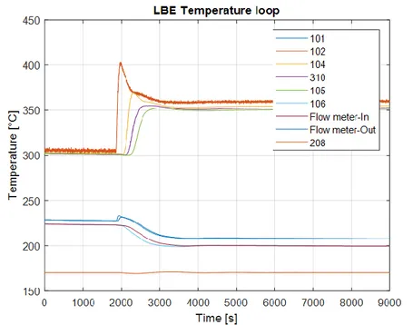
The time trend of the LBE temperature inside the main loop is illustrated in Figure 11. The water temperature at the inlet of the HX (TP208) was set to 170°C and the DACS regulates the pre-heater in order to have the desired value. The coldest part of the loop is situated between the HX outlet and the flow meter inlet (TP106 and TFM-In), the temperature increases few °C inside the thermal flow meter (TFM-out and TP101). The hottest part of the loop is downstream the FPS (TP102) and in the riser (TP104). Then the temperature decreases few °C going inside the expansion tank and for the thermal losses too (TP310 and TP105). After the transition, the cold temperatures decrease further, whereas the hot temperatures increase; resulting in higher temperature difference, as expected after the mass flow decrease.

(14)

Figure 11: LBE temperature inside the NACIE-UP loop, test ADP10.

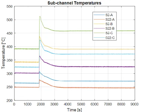
The details of the LBE and wall temperatures inside the FPS are reported from Figure 12 to Figure 17. In Figure 12, the section-averaged LBE temperature across the active region of the FPS and at the three monitored sections are reported. The LBE temperature inside the FPS increased just after the reduction of the gas flow rate and the resulting decrease in the LBE mass flow rate, but then stabilized to new values, once the new steady state took place. Figure 13 shows the LBE temperature in two monitored sub-channels, S2 and S22. S2 is located in the inner part of the bundle (inner rank), whereas S22 is placed in the second rank and exhibits colder temperatures. The temperature difference between the two sub-channels increased along the heated length, since the temperature profile was developing.

(15)

Figure 12: LBE average temperature inside the FPS, test ADP10.

Figure 13: LBE temperatures in sub-channels S2 and S22, at the three monitored sections (A, B, C), test ADP10.

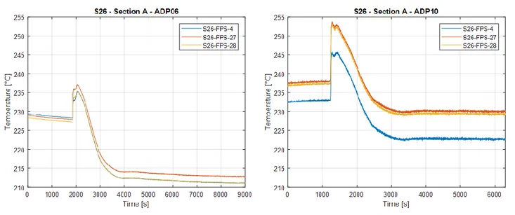
Figure 14, Figure 15 and Figure 16 illustrate the time trend of the LBE temperature in the centre of the sub-channel and at the pin walls related to the sub-sub-channels S2, S22, S26 and S33. Sub-sub-channels S26 and S33 are both located in the external rank, where the temperature is rather colder. Figure 14 refers to section A, located 38 mm after the beginning of the active region; Figure 15 shows the data related to section B, placed in the middle of the active region, whereas Figure 16 is related to section C, 562 mm after the beginning of the active region. The graphs on the left (a) of Figure 14,Figure 15 and Figure 16 report the time trend during the whole test of wall and sub-channels temperature of S2 and S22, whereas the graphs on the right (b)

(16)

show the analogous quantities for S26 and S33. The same range was adopted to plot Figures (a) and Figures (b) to better appreciate the temperature field inside the same section area. Indeed, the temperatures in the external region remains colder than the central one and this difference becomes more noticeable going from section A (Figure 14) to section C (Figure 16). In all the graphs, a peak in the wall and LBE temperature is noticeable when the gas transition took place, which caused a decrease of the LBE mass flow rate.

a) b)

Figure 14: Sub-channel and wall temperatures in sub-channels S2 and S22 section A (a)

and in sub-channels S26 and S33 (b), test ADP10.

a) b)

Figure 15: Sub-channel and wall temperatures in sub-channels S2 and S22 section B (a)

(17)

a) b)

Figure 16: Sub-channel and wall temperatures in sub-channels S2 and S22 section C (a)

Figure 17 shows the axial profile of the wall temperature of pin 3 in different moments between the first (t=1200 s) and the second (t=5000 s) steady state. The trend is not perfectly linear due to the influence of the wire around the pin. The slope of the trend increased suddenly at the beginning of the transient, then decreased slightly and stabilized to higher temperatures with respect to the first steady state due to the higher power to mass flow ratio.

Figure 17: Wall temperature along the active length of pin 3, during the transient of test ADP10.

The values of the main system parameters at the initial and final steady states of the test are reported in Table 3. When the gas flow rate was switched off from the initial value of 10Nl/min, the LBE mass flow rate decreased from the initial value of 2.56 kg/s to the final one of 1.31 kg/s. Consequently, the temperature

(18)

difference across the bundle increased, since the power was constant. Effective power was about 90% of the nominal one, power released in the “pre-active” was about 7-8%, the remaining part was probably dispersed radially outside the bundle.

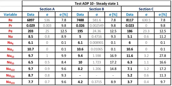
Table 4 and Table 5 report the computed non-dimensional number which characterized the test, respectively at the initial and final steady states. Reynolds, Prandtl and Péclét numbers tended to increase or decrease from section A to section C due to the temperature dependence of these quantities, since the LBE average temperature increase with the height. The overall Nusselt number tended to decrease with the axial position and the computed values seem to be fitted better by the Kazim-Carelli correlation (NuK). The Ushakov correlation better fits the value of the local Nussel number of the central sub-channels (S2, S5 and S22), which are representative of the infinite-lattice channel. Nu in peripheral sub-channel tended to be smaller, being strongly affected by the presence of the external wrapper.

Table 3: Integral parameters for the initial and final steady state of test ADP10.

Table 4: FPS non-dimensional variables at the initial steady state of test ADP10. Test ADP 10

Variable Data σ σ [%] Data σ σ [%]

Mgas [Nl/min] 10 0.5 5 0.1 0 2.8

Mlbe [kg/s] 2.56 0.07 2.9 1.31 0.04 2.9

∆TFPS [°C] 72 0.7 0.9 140.6 0.3 0.2

Qnom [W] 3.00E+04 50 0.2 3.00E+04 44 0.1

Qeff [W] 2.71E+04 1053 3.9 2.70E+04 1010 3.7

Qpre [W] 2236 403 18 2339 217 9.3

Qtfm [W] 1915 3 0.2 1644 4 0.3

Steady state 1 Steady state 2

Variable Data σ σ [%] Data σ σ [%] Data σ σ [%]

Re 6897 536 7.8 7488 581.6 7.8 8117 630.5 7.8 Pr 0.029 0.003 9.8 0.026 0.002549 9.8 0.023 0 9.8 Pe 203 25 12.5 195 24.36 12.5 186 23.3 12.5 Nu 8.5 0.8 8.9 5 0.4716 9.3 5.1 0.6 11.2 NuK 6.1 0 0.1 6.1 0.008901 0.1 6 0 0.1 NuU 10.7 0 0.1 10.6 0.01065 0.1 10.6 0 0.1 NuS2 9.7 1 9.9 9.4 1.598 16.9 11.6 3.2 27.8 NuS5 6.5 0.5 8.4 10 1.723 17.2 6.3 1.1 16.6 NuS22 9.7 0.9 9.6 8.2 1.206 14.8 7.1 1.2 17.2 NuS26 8.7 0.8 9.3 - - - 5.2 0.6 11.3 NuS33 7.7 0.7 9.6 4.2 0.3715 8.9 3.7 0.4 9.7

Test ADP 10 - Steady state 1

(19)

Table 5: FPS non-dimensional variables at the final steady state of test ADP10.

3.3 ADP06 experimental results

The test ADP06 consisted in gas-lift transition, whereas the FPS power was maintained constant at the nominal power of 30 kW. The power in test ADP06 was distributed among the 7 central pins (pins from 1 to 7), as it was shown in Figure 4. The total electrical power (30 kW) was the same of test ADP10 but, being divided in less number of pins, the corresponding nominal wall heat flux is higher: ''

.

2

w

q



347 1 kW m

in ADP06 versus

q

_w''



127 9 kW m

.

2 in ADP10. Local effects will be analysed in this section: the temperature distribution inside the bundle will be necessary incongruous between the two tests, due to the different pins wall heat flux. The trend of the integral parameters will be also examined and compared with the ones of test ADP10 in this section.

As for test ADP10, the nominal gas flow rate was initially set at 10Nl/min and then decreased to 0 Nl/min also in test ADP06. The experimental trend of the Ar-3%H2 flow rate and of the FPS power (boundary conditions of the test) were reported in Section 2.2 (Figure 5 and Figure 6).

Looking at the results of test ADP10, Figure 18 (a) shows the time trend of the LBE mass flow rate and Figure 18 (b) catches time-zoom of the same plot, during the gas flow transition (t=1800-2500 s). After that the gas injection in the riser was switched off, the LBE mass flow rate underwent a sudden decrease and soon after stabilized to lower value with respect to the starting steady condition.

a) b)

Re 3457 268 7.7 4060 315 7.7 4647 360 7.7 Pr 0.03 0.003 9.8 0.024 0.002 9.8 0.019 0.002 9.8 Pe 105 13 12.5 97 12 12.5 89 11 12.5 Nu 6.9 0.5 7.9 4.4 0.3 7.6 4.1 0.3 7.8 NuK 5.4 0 0.2 5.4 0 0.2 5.3 0 0.2 NuU 9.9 0 0.1 9.9 0 0.1 9.8 0 0.1 NuS2 8.2 0.7 8.2 9.1 0.8 8.7 13.9 1.8 12.9 NuS5 5.3 0.4 7.7 9.6 0.9 9.2 5.5 0.5 8.7 NuS22 8.7 0.7 8.2 6.7 0.6 8.4 5.9 0.5 8.5 NuS26 5.9 0.5 8.1 - - - 3.3 0.3 7.8 NuS33 6.3 0.5 8.4 3.6 0.3 7.6 3.1 0.2 7.7

(20)

The time trend of the LBE temperature inside the main loop is illustrated in Figure 19. The water temperature at the inlet of the HX (TP208) was set to 170°C and the DACS regulates the pre-heater in order to have the desired value. The coldest part of the loop is situated between the HX outlet and the flow meter inlet (TP106 and TFM-In), the temperature increases few °C inside the thermal flow meter (TFM-out and TP101). The hottest part of the loop is downstream the FPS (TP102) and in the riser (TP104). Then the temperature decreases few °C going inside the expansion tank and for the thermal losses too (TP310 and TP105). After the transition, the cold temperatures decreased slightly, whereas the hot temperatures increase; resulting in higher temperature difference, as expected after the mass flow decrease. The LBE temperature at the HX outlet was about 223°C in the first part of the test and decreased to about 200°C in the second part. The temperature at the FPS outlet went from about 305°C (first steady state) to 360 °C (second steady state).

Figure 20 illustrates the section-averaged LBE temperature across the active region of the FPS and at the three monitored sections. The LBE temperature inside the FPS increased just after the reduction of the LBE mass flow rate, but then stabilized to new values. Figure 21 shows the LBE temperature in two monitored sub-channels, S2 and S22. S2 is in the inner part of the bundle (inner rank), whereas S22 is placed in the second rank. The temperature difference between the two sub-channels increased along the heated length, since the temperature profile is developing. In particular, the temperature in S2, which is the inner rank (closer to the active region), increases much more with respect to the temperature in S22. Moreover, the LBE temperature in S2 at section B resulted higher than LBE temperature in S22 at section C, which is placed closer to the outlet of the bundle. This data proves that the sub-channel S22 is affected by the configuration of active pins, since pin 16 was switched off.

(21)

Figure 20: LBE average temperature inside the FPS, test ADP06.

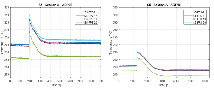
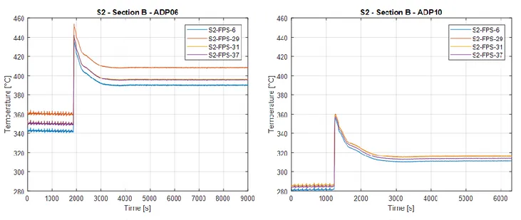
The following figures (from Figure 22 to Figure 36) show the time trend of the pins wall temperatures and of the LBE temperature at the centre of the sub-channels. Each figure is related to one sub-channel in one of the three monitored section. Time trends of test ADP06 are reported in sub-figures (a), whereas sub-figures (b) display the corresponding plot during test ADP10 in order to compare the two tests and highlight the effect of the different power distribution. For a better comparison the same range was used for each sub-figure (a), with the corresponding (b). At first sight, it is possible to notice that sub-channels S2, S5 and S22 are hotter in case of ADP06, whereas S26 and S33 are colder with respect to test ADP10. As a matter of fact

(22)

the wall heat flux is higher in the central pins in ADP06 with respect to ADP10, but the flux is zero in the external pins.

Some considerations can be pointed out looking at the figures below. In sub-channel S22 (Figure 24, Figure 29 and Figure 34), one of the wall temperatures (TC-FPS-26 TC-FPS-39 and TC-FPS-52) remained always below the relative sub-channel temperature (TC-FPS-03 TC-FPS-08 and TC-FPS-13), since are relative to pin 16, which was off during ADP06. In sub-channel S2 and S5, especially in section B and C, it is noticeable that the wall temperatures relative to pin 1 (TC-FPS-29 TC-FPS-30, TC-FPS-42, TC-FPS-43) were typically higher than other wall temperatures, since pin 1 is the innermost one. In the external sub-channels S26 and S33, the wall and sub-channel temperatures are very similar in section A, since the pins are not heated. Nevertheless, the difference between wall and sub-channel temperatures became evident in section B and C because the temperature profile developed along the active length.

a) b)

Figure 22: Sub-channel and wall temperatures in sub-channels S2 section A, during ADP06 (a) and ADP10 (b).

a) b)

(23)

a) b)

(24)

a) b)

Figure 27: Sub-channel and wall temperatures in sub-channels S2 section B, during ADP06 (a) and ADP10 (b).

(25)

a) b)

(26)

a) b)

(27)

a) b)

Figure 32: Sub-channel and wall temperatures in sub-channels S2 section C, during ADP06 (a) and ADP10 (b).

a) b)

(28)

a) b)

(29)

a) b)

Figure 37 shows the axial profile of the wall temperature of pin 3 in different moments between the first (t=1800s) and the second (t=9000s) steady state. Considering test ADP06, pin 3 is in a particular position because it is included in the heated part of the bundle but it is surrounded by three active pins and three pins turned off. Also, the influence of the wire around the pin affected the wall temperature measured along the generatrix of the rod, resulting in a not perfectly linear trend. The wall temperature increased suddenly at the beginning of the transient, then decreased slightly and stabilized to higher temperatures with respect to the first steady state due to the higher power to mass flow ratio.

The values of the main system parameters at the initial and final steady state of the test are reported in Table 6. When the gas flow rate was switched off from the initial value of 10Nl/min, the LBE mass flow rate

(30)

decreased from the initial value of 2.66 kg/s to the final one of 1.33 kg/s. The analogous values in test ADP10 were respectively 2.56 kg/s and 1.31 kg/s. It can be noticed that, at the same power level, the LBE mass flow in the two test cases were very similar. The temperature difference across the bundle increase in the second part of the test, due to the lower mass flow rate. Effective power was about 90% of the nominal one in the first part of the test, but decreased slightly in the second part (about 85%), maybe due to large losses at relatively high heat flux and low LBE mass flow rate.

Table 7 and Table 8 show non-dimensional number computed for test ADP06, respectively at the initial and final steady states. Reynolds, Prandtl and Péclét numbers tended to increase or decrease from section A to section C due to the temperature dependence of these quantities, since the LBE average temperature increased with the height. The overall Nusselt number was not computed because its definition is strongly affected by the LBE temperature in the external rank ,which, in this case, is particularly cold due to the peculiar power distribution. In such configuration, the definition of the local Nu cannot be applied to sub-channels S22, S26 and S33, which present one or more pins around the channel that were off. However, local Nu in sub-channels S2 and S5 are rather smaller with respect to test ADP10, so also central pins are relatively affected by the power distribution and the consequent temperature distribution in the bundle.

Table 7: FPS non-dimensional variables at the initial steady state of test ADP06.

Table 8: FPS non-dimensional variables at the final steady state of test ADP06. Test ADP 06

Mgas [Nl/min] 10 0.5 5 0 0 2.8

Mlbe [kg/s] 2.66 0.08 2.9 1.33 0.04 2.9

∆TFPS [°C] 68.4 0.8 1.1 130.1 0.5 0.4

Qnom [W] 3.00E+04 50 0.2 3.00E+04 51 0.2

Qeff [W] 2.68E+04 1052 3.9 2.54E+04 952 3.7

Qpre [W] 2508 438 17.5 2675 230 8.6

Qtfm [W] 1933 3 0.2 1652 4 0.3

Re 7236 562 7.8 7885 612 7.8 8440 655 7.8 Pr 0.029 0.003 9.8 0.026 0.002 9.8 0.023 0.002 9.8 Pe 210 26 12.5 201 25 12.5 194 24 12.5 NuK 6.2 0 0.1 6.1 0 0.1 6.1 0 0.1 NuU 10.7 0 0.1 10.7 0 0.1 10.6 0 0.1 NuS2 3.2 0.3 8.4 3.1 0.4 11.4 2.2 0.2 10.3 NuS5 2.2 0.2 7.8 4.8 0.7 13.9 3.2 0.4 13.3

Section A Section B Section C

Re 3522 273 7.7 4094 317 7.7 4644 360 7.7 Pr 0.03 0.003 9.8 0.024 0.002 9.8 0.02 0.002 9.8 Pe 107 13 12.5 99 12 12.5 92 11 12.5 NuK 5.5 0 0.2 5.4 0 0.2 5.3 0 0.2 NuU 10 0 0.1 9.9 0 0.1 9.8 0 0.1 NuS2 2.8 0.2 7.6 3.3 0.3 7.7 2.3 0.2 7.8 NuS5 1.9 0.1 7.5 4 0.5 12.1 2.7 0.2 9

(31)

3.4 ADP07 experimental results

The test ADP07 concerned a gas-lift transition, whereas the FPS power was maintained constant at the nominal power of 38 kW. During test ADP07, the power was distributed among 9 pins corresponding to two adjacent triangular sectors over the bundle section (pins 1, 2, 6, 7, 8, 9, 17, 18 and 19), as it was illustrated inFigure 7. The total electrical power was set to 38 kW with the aim to have pin-wall heat flux comparable to the values of test ADP06. Nominal wall heat flux in test ADP07 was about ''

.

2

w

q



342 0 kW m

, whereas the nominal value in test ADP06 was about

q

_w''



347 1 kW m

.

2. The local effects of this specific power distribution will be analysed in this section. The temperature distribution inside the bundle will be necessary dissymmetric as the boundary conditions of the test are. As in precedent tests, the nominal gas flow rate was initially set at 10Nl/min and then decreased to 0 Nl/min. The experimental trend of the Ar-3%H2 flow rate and of the FPS power (boundary conditions of the test) were reported in Section 2.3, in Figure 8 and Figure 9. The experimental results regarding the LBE mass flow rate, obtained during test ADP07, are shown in Figure 38: sub-figure (a) displays the time trend over the total duration of the test and sub-figure (b) a zoom in the time trend during the gas flow rate transition.

a) b)

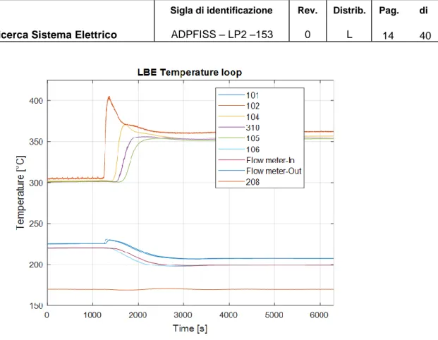
The time trend of the LBE temperature inside the main loop is illustrated in Figure 39. The water temperature at the inlet of the HX (TP208) was set to 170°C and the DACS regulates the pre-heater in order to have the desired value. The coldest part of the loop is situated between the HX outlet and the flow meter inlet (TP106 and TFM-In), the temperature increases few °C inside the thermal flow meter (TFM-out and TP101). The hottest part of the loop is downstream the FPS (TP102) and in the riser (TP104). The LBE temperature at the HX outlet was about 233°C in the first part of the test and decreased to about 211°C in the second part. The temperature at the FPS outlet increased from about 320°C (first steady state) to 384 °C (second steady state).

(32)

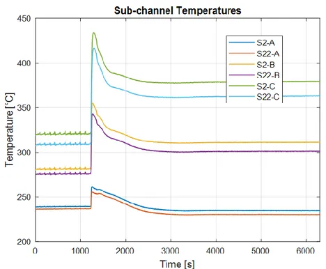
The details of the LBE and wall temperatures inside the FPS are reported from Figure 40 to Figure 44. Figure 40 illustrates the section-averaged LBE temperature at the inlet, at the outlet and at the three monitored sections, whereas Figure 41 shows the LBE temperature in the center of sub-channels S2 and S22. During the test, all the pins relative to channel S2 (pins 1, 2 and 7) were on, whereas for sub-channel S22, just one out of three pins relative to the sub-sub-channel was switched on (pin 6). Indeed, LBE temperature in S22 remained considerably lower with respect to S2. Even, LBE temperature in S2 section B is almost 100°C larger than LBE temperature in S22 section C, showing the remarkable asymmetry of the heating.

(33)

Figure 42, Figure 43, Figure 44 display the time trend of the LBE temperature in the centre of the sub-channel and at the pin walls related to the sub-sub-channels S2, S22, S26 and S33. Figure 42 refers to section A, located 38 mm after the beginning of the active region; Figure 43 shows the data related to section B, placed in the middle of the active region, whereas Figure 44 is related to section C, 562 mm after the beginning of the active region. Sub-figures (a) are relative to sub-channels S2 and S22 and sub-figures (b) are relative to sub-channels S26 and S33. As mentioned, all the pins related to S2 were on during the test, so the sub-channel TC of S2 was “inside” the active sectors. Regarding sub-channel S22, pin6 was switched on but pins 15 and 16 were off, the sub-channel TC is located outside the active region of the bundle. For what concerns channel S26, the pins related to it (pins 18 and 19) were on during the test and sub-channel TC was surrounded by active pins. Instead, pin 9 (the one relative to sub-sub-channel S33) was active during the test, but the sub-channel TC of S33 was outside the active sector, being adjacent to the non-active region too. The same range was adopted to plot Figures (a) and Figures (b) to better appreciate the temperature field inside the same section area. It is evident that most of the temperatures measured in S22 were colder than the temperatures in heated sub-channels S2, S26 and S33. Wall temperature relative to pin 6, which is the active one belonging to S22, is hotter than the other wall temperature of S22. In S2, it was possible to notice that, in section B, the wall temperature related to pin1 (TC-FPS-29) was colder than the other pin wall temperatures (TC-FPS-31 and TC-FPS-37) and also colder of the sub-channel temperature (TC-FPS-060). In S2 section C, the sub-channel temperature (TC-FPS-11) was even hotter than all the wall temperatures (TC-FPS-42, TC-FPS-44 and TC-FPS-50). Temperatures of sub-channels S26 and S33 remained slightly lower than the ones relative to S2, maybe because located in the external rank, and so affected by the presence of the external wrapper. From Figure 44, it is possible notice the large temperature difference on a transversal section, which exceeded 200° in the second part of the test.

(34)

a) b)

Figure 42: Sub-channel and wall temperatures in sub-channels S2 and S22 section A (a)

a) b)

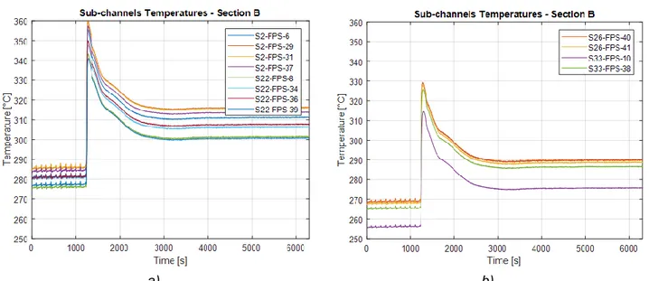
Figure 43: Sub-channel and wall temperatures in sub-channels S2 and S22 section B (a)

(35)

a) b)

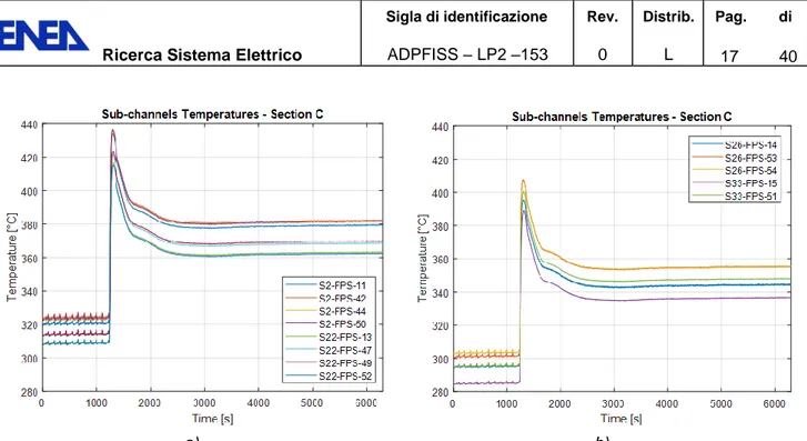
Figure 44: Sub-channel and wall temperatures in sub-channels S2 and S22 section C (a)

Figure 45 shows the axial profile of the wall temperature of pin 3 in different moments between the first (t=1200 s) and the second (t=4800 s) steady state. During the test ADP07, pin 3 was outside the heated area but was surrounded by two active pins (1 and 2). The presence of the wire spacers could affect the mixing of the flow and its cooling function, so that the wall temperature measured along the generatrix of the pin3 presented a non-linear trend. The wall temperature increased suddenly at the beginning of the transient, then decreased slightly and stabilized to higher temperatures with respect to the first steady state due to the higher power to mass flow ratio.

(36)

The values of the main system parameters at the initial and final steady state of the test are reported in Table 9. When the gas flow rate was switched off from the initial value of 10Nl/min, the LBE mass flow rate decreased from the initial value of 3.07 kg/s to the final one of 1.60 kg/s. Consequently, the temperature difference across the bundle increased from about 80°C to 147°C.

Table 10 and Table 11 report the computed non-dimensional numbers for test ADP07, respectively at the initial and final steady states. Reynolds decreased from about 104 to 5·103, going from the first to the second steady state, and Péclét from about 200 to about 100, remaining the Prandtl number between0.2 and 0.3 during the whole duration of the test. Regarding the Nusselt number, it was not possible to compute the average Nusselt as defined in Section 3.1.1, due to the asymmetric configuration of the heated area. In such configuration, the definition of the local Nu was applied to sub-channel S26, which had all the pins of the sub-channel on. Sub-channel S2 had all the pins around the channel on, but was highly affected by the presence of cold pins adjacent pin1, as analyzed before. However, local Nu in sub-channels S26 presented quite small values, maybe because affected by the external wrapper.

Table 10: FPS non-dimensional variables at the initial steady state of test ADP07. Test ADP 07

Mgas [Nl/min] 10 0.5 5.5 0.1 0 2.8

Mlbe [kg/s] 3.07 0.09 2.9 1.6 0.05 2.9

∆TFPS [°C] 79.4 0.8 1 146.6 0.8 0.6

Qnom [W] 3.80E+04 40 0.1 3.80E+04 51 0.1

Qeff [W] 3.57E+04 1390 3.9 3.42E+04 1288 3.8

Qpre [W] 4165 497 11.9 4595 311 6.8

Qtfm [W] 1960 3 0.1 1680 4 0.2

Test ADP 07

Mgas [Nl/min] 10 0.5 5.5 0.1 0 2.8

Mlbe [kg/s] 3.07 0.09 2.9 1.6 0.05 2.9

∆TFPS [°C] 79.4 0.8 1 146.6 0.8 0.6

Qnom [W] 3.80E+04 40 0.1 3.80E+04 51 0.1

Qeff [W] 3.57E+04 1390 3.9 3.42E+04 1288 3.8

Qpre [W] 4165 497 11.9 4595 311 6.8

Qtfm [W] 1960 3 0.1 1680 4 0.2

Re 8642 671 7.8 9533 740 7.8 10220 793 7.8 Pr 0.028 0.003 9.8 0.024 0.002 9.8 0.021 0.002 9.8 Pe 238 30 12.5 226 28 12.5 217 27 12.5 NuK 6.3 0 0.1 6.3 0 0.1 6.2 0 0.1 NuU 10.9 0 0.1 10.8 0 0.1 10.8 0 0.1 NuS26 3.6 0.3 7.8 - - - 2.5 0.2 9.2

(37)

Table 11: FPS non-dimensional variables at the final steady state of test ADP07.

Re 4432 343 7.7 5256 407 7.7 5904 457 7.7 Pr 0.028 0.003 9.8 0.022 0.002 9.8 0.018 0.002 9.8 Pe 125 16 12.5 114 14 12.5 106 13 12.5 NuK 5.6 0 0.2 5.5 0 0.2 5.4 0 0.2 NuU 10.1 0 0.1 10 0 0.1 9.9 0 0.1 NuS26 2.6 0.2 7.9 - - - 1.6 0.1 7.9

(38)

4 Conclusions

This document describes the experimental campaign performed with the NACIE-UP (NAtural CIrculation Experiment-UPgrade) facility located at the ENEA Brasimone Research Center (Italy) in the framework of the Programmatic Agreement (Accordo di Programma - AdP) between the Italian Ministry of the Economic Development (MSE) and ENEA. The campaign focused on system and local thermal-hydraulic analysis, respectively on the LBE loop of the facility and its main test section, composed by a prototypical 19-pins, wire-spaced, fuel pin simulator. The main objective of this work was to perform mass flow rate transient tests, with transition from forced to natural circulation flow, with fuel pin simulator characterized by a power distribution uniformly distributed over the bundle section in order to evaluate the effects of this non-uniformity on the local temperatures and, potentially, on the overall system behavior.

A first test, with power uniformly distributed, was performed to have reference case for comparison. As expected, the external part of the bundle was colder, and the local Nu exhibited lower values in the external sub-channels (S26 and S33) with respect to the internal ones (S2, S5 and S22). A peak on the FPs temperature occurred when the gas transition took place, causing a decrease of the LBE mass flow rate. The second test was characterized by the same power level of the first one, but distributed among less number of pin, which had, consequently, higher wall heat flux on the active pins. Regarding the overall system main parameters, it was noticed that the LBE mass flow rate and the loop temperatures in the two test cases were very similar. Concerning the local temperatures, sub-channels S2, S5 and S22 were hotter in the second test with respect to the first, whereas S26 and S33 were obviously colder, being the related pins turned off during the second test. The effect of the non-uniform power distribution could be observed in sub-channel S22, where one of the wall temperatures (TC-FPS-26 TC-FPS-39 and TC-FPS-52) remained always below the relative sub-channel temperature (TC-FPS-03 TC-FPS-08 and TC-FPS-13), being relative to pin 16, which was off during the test. Also the third test was characterized by power distribution localized in a limited part of the bundle, specifically in two triangular sections (two sixth) of the hexagonal configuration. The power value was chosen in order to have pin-wall heat flux comparable with the second test. During this third test, temperatures measured in S22 were colder than the temperatures in heated sub-channels S2, S26 and S33. Non-conventional behaviour was noticed in S2: in section C, the sub-channel temperature (TC-FPS-11) was hotter than all the wall temperatures (TC-FPS-42, TC-FPS-44 and TC-FPS-50). Also, temperatures of sub-channels S26 and S33 remained slightly lower than the ones relative to S2, maybe because located in the external rank, and so affected by the presence of the external wrapper.

The obtained experimental data provided useful information for the characterization of the bundle and the computation of the heat transfer coefficient. Moreover, the collected system data can be used to qualify STH codes, whereas the local fuel bundle data, especially the ones from dissymmetric tests can be useful for the validation and benchmarking of CFD codes and coupled STH/CFD methods for HLM systems.

(39)

Acronyms and definitions

Acronym Definition

CFD Computational Fluid Dynamics DACS Data Acquisitions and Control System

FPS Fuel Pin Simulator

HLM Heavy Liquid Metal

HX Heat eXchanger

LOFA Loss Of Flow Accident LBE Lead-Bismuth Eutectic

NACIE-UP NAtural CIrculation Experiment- UPgraded

O.D. Outer Diameter

STH System Thermal-Hydraulic

TC Thermocouple

Nomenclature

Symbol Definition

A

Flow area

Q

_nom Nominal power

c

p Specific heat capacity

Q

pre Power released in pre-active region

D

Pins diameter

Re

Reynolds number

D

H Hydraulic diameter

t

Time

k

LBE conductivity

T

_ac Acquired Temperature

k

ss Stainless steel conductivity

T

b Bulk Temperature

L

active Active length of the pins

T

in FPS inlet Temperature

M

Number of pins

T

_out FPS outlet Temperature

m

Mass flow rate

T

_sc LBE sub-channel Temperature

Nu

Nusselt number

T

_w Wall Temperature

Pe

Péclet number

Pr

Prandtl number



_g Distance between the center of the TC and

the cladding outer surface

q

w

’’

Wall heat flux

ρ

LBE density

(40)

References

[1] I. Di Piazza, M. Angelucci, R. Marinari, M. Tarantino, and N. Forgione, “Heat transfer on HLM cooled wire-spaced fuel pin bundle simulator in the NACIE-UP facility,” Nucl. Eng. Des., vol. 300, pp. 256– 267, 2016.

[2] R. S. Elettrico, I. Di Piazza, A. Del Nevo, and M. Tarantino, “UPGRADE AND EXPERIMENTAL TESTS IN THE HLM FACILITY NACIE-UP WITH A PROTOTYPICAL THERMAL FLOW METER List of contents,” 2016.

[3] M. D. Kazimi, M.S., Carelli, “Clinch River Breeder Reactor Plant heat transfer correlation for analysis of CRBRP assemblies.,” 1976.

[4] P. A. Ushakov, A. V. Zhukov, and N. M. Matyukhin, “HEAT TRANSFER TO LIQUID METALS IN REGULAR ARRAYS OF FUEL ELEMENTS.,” High Temp., vol. 15, no. 5, 1977.

[5] N. E. Agency, “Handbook on Lead-bismuth Eutectic Alloy and Lead Properties, Materials Compatibility , Thermal- hydraulics and Technologies,” Nucl. Sci., pp. 647–730, 2015.

Test di caratterizzazione termo-fluidodinamica sull’impianto NACIE

Titolo