Performance analysis of queueing systems with resequencing

(1)

UNIVERSIT `

A DEGLI STUDI DI SALERNO

Dipartimento di Matematica

Dottorato di Ricerca in Matematica XIV ciclo - Nuova serie

Performance analysis of

queueing systems with

resequencing

Candidato: Caraccio Ilaria

Coordinatore: Chiar.ma Prof.ssa Patrizia Longobardi

Tutor: Chiar.mo Prof. Ciro D’Apice

Cotutor: Prof.ssa Rosanna Manzo

(2)

(3)

List of Figures

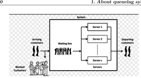
1.1 A queueing system. . . 10

2.1 Scheme of the model. . . 15

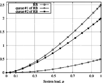
2.2 Mean number of customers. . . 39

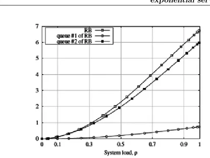
2.3 Variance of the number of customers. . . 40

2.4 Coeﬃcients of correlation. . . 41

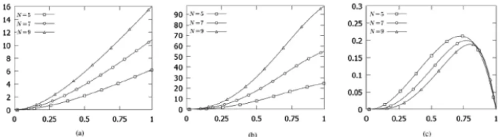
3.1 Dependence on load ρ/N of (a) mean number of cus-tomers in reordering buffer, (b) variance of number of customers in reordering buffer, (c) correlation on the number of customers in queue and reordering buffer. . . 56

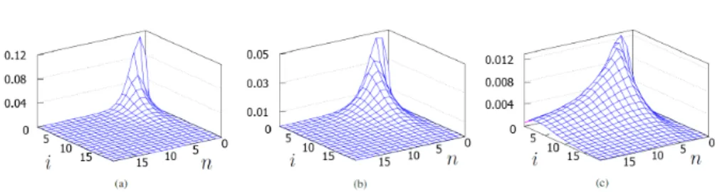
3.2 Join stationary distribution pπ;i (a) ρ/5 = 0.5, (b) ρ/5 = 0.7, (c) ρ/5 = 0.9. . . . 57

4.1 Mean and variance of the number of the requests in the reordering buffer and the coefficient of correla-tion of the number of the requests in the reordering buffer and in the buffer. . . 80

4.2 Moments of the arrival time of the requests in the system and in the reordering buﬀer. . . 81

4.3 Moments of the distribution of the mean time of the arrival of the requests in the system and in the reordering buﬀer for both systems with a diﬀerent values of the parameters of the MAP process and the same values for the parameters of the service process. . . 82

(6)

(7)

1

Background, literature review and

mo-tivation

The service sector lies at the heart of industrialized nations and continues to serve as a major contributor to the world economy. Over the years, the service industry has given rise to an enor-mous amount of technological, scientific, and managerial chal-lenges. Among all challenges, operational service quality, service efficiency, and the tradeoffs between the two have always been at the center of service managers’ attention and are likely to be so more in the future. Queueing theory attempts to address these challenges from a mathematical perspective. Every service station of a queueing network is characterized by two major components: the external arrival process and the service process. The external arrival process governs the timing of service request arrivals to that station from outside, and the service process concerns the duration of service transactions in that station. These are then fused with a routing process among stations to form the structure of the queue-ing network. Since the arrival, service, and routqueue-ing processes are usually stochastic by nature, the study of service networks involves probabilistic analysis, which is the subject of queueing theory. Many distributed applications, such as voice data transmission, remote computations, and database manipulations, information integrity require that data exchanges between different nodes of a system be performed in a specific order. Recently, multipath rout-ing has received some attention in the context of both wired and wireless communication networks. By sending data packets along different paths, multipath routing can potentially help balance the traffic load and reduce congestion levels in the network, thereby re-sulting in lower sojourn time. Under multipath routing, since con-secutive packets travel possibly along different paths from source to destination, they can easily be received out-of-sequence at the destination. If the application requires packets to be processed in the order in which they were sent, then disordered packets have to wait an additional amount of time, known as the resequencing delay, before being consumed. Packet mis-ordering occurs in the

(8)

following two transmission scenarios. In the first scenario, multi-ple (or parallel) routes between the transmitter-receiver pair are utilized to send data packets to increase the data transmission rate. However, a packet transmitted along one route may experi-ence a time delay that is different from that along another route. Consequently, a packet that was sent by the transmitter earlier than another may arrive at the receiver later, resulting in packet mis-ordering at the receiver end. In the second scenario, packets may be lost or erroneously received due to channel degradation, congestion or any network hardware malfunction along a route, in which case they have to be retransmitted for error-free data transmissions via a retransmission scheme, such as the selective repeat automatic repeat request protocol (SR-ARQ). Retransmis-sion of corrupted or lost packets can cause packets to be received out-of-order at the receiver as well. Note that the second scenario happens when there is one single channel between the transmitter and the receiver. In practice, many applications require that the packets are received in the same order from which they were sent. For such applications, the receiver has to buffer the mis-ordered packets in a resequencing buffer, resequence them repeatedly, and deliver them in the corrected order. This process is referred to as packet resequencing. The resequencing issue in simultaneous pro-cessing systems, where the order of customers (jobs, units, etc.) upon arrival has to be preserved upon departure, is a crucial theme in the queueing theory. Queueing-theoretic approach to resequenc-ing problem implies that the system under consideration is rep-resented as interconnected queueing systems/ networks. Various analytical methods and models have been proposed to study the impacts of resequencing. A general survey of queueing theoretic methods and early models for the modeling and analysis of paral-lel and distributed systems with resequencing can be found in [7]. Survey on the resequencing problem that covers period up to 1997 can be found in [8]. In [1] a continuous-time M/M/2 queueing sys-tem, with two heterogeneous servers, a routing policy with variable routing position, is analyzed with the objective of minimizing the sum of the queueing delay and resequencing delay and of

(9)

comput-3

ing the total expected end-to-end delay (including the resequenc-ing delay). In [2] the effect of fixed delay on the optimal traffic split is studied for a continuous-time system of two end nodes with two parallel M/M/1, in order to minimize the total end to end delay (including the resequencing delay) in a high speed environment. In [3] a continuous-time 2-M/M/1 network is considered and the asymptotic expression of the probability that there are n packets in reordering buffer as n became large is computed, in order to avoid a reduced data throughput caused by overflow of the resequencing queue, a large enough buffer size of the resequencing queue has to be configured. In [4] a distributed system consisting of two par-allel heterogeneous single server M/M/1 queues is analyzed. It is assumed that a total number of C different classes arrive at the source node. The resequencing delay when C = 1 is evaluated, and the result is then extended to the case of a single class with interfering traffics (that is an additional stream of customers), and in the case of two-class and multiple class systems. In [5] a M/M/2 system is considered, in which servers are parallel, heterogeneous and exponential and the customers are released from the system after service completion according to their arrival order. The cus-tomers, which are delayed due to resequencing, have to wait in a resequencing queue. The attention is limited to fixed-position routing policies which route customers to server 1 only from the head of queue Q, and to server 2 only from a fixed position J , J ≥ 2, where position J means the Jth customer among those in server 1 and in queue Q. The existence of an optimal stationary policy is shown: the faster service is kept active as long as the service queue is not empty. In [6] a virtual circuit from node S to node D connected by m links in parallel, whose arrival process is general and the service times are exponentially distributed, is investigated. An important property of a virtual circuit is that it delivers packets at the destination in the same sequence as they are received at the source. A packet arriving at S has to wait if all links are busy. The distribution of the total delay for the G/M/m queueing system model, the distribution of the resequencing delay for the G/M/m queueing system model, the expectation of the

(10)

resequencing delay for the G/M/m queueing system model, the distribution of the total delay for the M/M/m, the M/HK/∞ and the G/M/∞ queueing system model is obtained. The resequenc-ing has also been studied in system in which the arrivals follow a more complicated process: the Markovian arrival process (MAP). In [9] a MAP/M/2/K queueing model in which messages should leave the system in the order in which they entered into the sys-tem is considered. In the case of infinite resequencing buffer, the steady-state probability vector is shown to be of matrix-geometric type. The total sojourn time of an admitted message into the sys-tem is shown to be of phase type. Efficient algorithmic procedures for computing various performance measures are given. In [10] a two-server finite capacity queuing model in which messages should leave the system in the order in which they entered the system, is studied. Messages arrive according to a Markovian arrival process and any message finding the buffer full is considered lost. Out-of-sequence messages are stored in a (finite) buffer and may lead to blocking when a processed message cannot be placed in the buffer. Using matrix-analytic methods, the system is analyzed in steady state. It is shown that the stationary waiting time distri-butions of an admitted message in the queue and in the system as well as the time spent in the service facility follow phase-type distributions. The departure process is characterized as a Batch Markovian Arrival Process. The system performance measures such as system idle probability, server idle and server blocking probabilities, throughput, mean number of messages in primary and in resequencing buffers, rate of departure, average batch size of departure are derived analytically. In [15] a model where the disordering is caused by multipath routing is analyzed. Packets are generated according to a Poisson process. Then, they arrive at a disordering network (DN) modeled by two parallel M/M/1 queues, and are routed to each of the queues according to an inde-pendent Bernoulli process. A resequencing buffer follows the DN. In such a model, the packet resequencing delay is known. How-ever, the size of the resequencing queue (RSQ) is unknown. The probability for the large deviations of the queue size is analyzed.

(11)

5

Other systems with resequencing have been studied in [16], [17], [18], [20], [19].

(12)

Purpose of the thesis

The main objective of this research is to find the stationary charac-teristics of M/M/3/∞, M/M/∞/∞ and MAP/PH/2/∞ queueing systems with reordering buﬀer of infinite capacity.

In the M/M/3/∞ customers in reordering buffer may form two separate queues and focus is given to the study of their size dis-tribution. These two queues are labeled as queue 1 and queue 2. In queue 1 there are customers that are waiting for two customers that are still in service, while in queue 2 there are customers that are waiting for one customer that is still in service. Expressions for joint stationary distribution are obtained both in explicit form and in terms of generating functions. When the parameter of ser-vice µ is equal to one and the parameter of arrival λ is between 0.1 and 2.5, numerical examples are given for the mean number of customers in reordering buffer (RB) (queue 1 and queue 2), for the variance of number of customers in RB (queue 1 and queue 2), the coefficient of correlation between queue 1 and queue 2, between queue 1 and RB, between queue 2 and RB.

In the M/M/∞/∞ we propose a new problem statement for sys-tems with resequencing that are modeled by multiserver queues followed with infinite resequencing buffer. Focus is given to the study of joint stationary distribution of the total number of cus-tomers in queue and total number of cuscus-tomers in reordering buffer. Using developed analytical methods there was obtained the system of equilibrium equations which allows recursive com-putation of joint stationary distribution of the total number of customers in buffer and servers and total number of customers in RB.

In MAP/PH/2/∞ we have a queueing system with 2 servers, in which the capacity of the collecting buffer and the reordering buffer is infinite. The type distribution of both two servers is ”the phase distribution” (PH), while the arrivals follow Markovian arrival pro-cess. We introduce a recurrent algorithm to calculate the simul-taneous stationary distribution of the number of the requests at servers, in the collecting buffer and in the reordering buffer. The

(13)

7

stationary distribution of the arrival time in the system and in the reordering buﬀer are calculated with the Laplace-Stieltjes trans-form.

(14)

(15)

Chapter 1 About queueing system

For an accurate description of a queueing system, we need to pro-vide its following basic elements:

1. The input process. It refers to the arrivals to the system. It describes the distribution and dependencies of the interar-rival times. The most common input process is the Poisson process.

2. The service mechanism. The basic characteristics of the ser-vice mechanism include the number of parallel servers, their identity (homogeneous or heterogeneous, their service speed etc.) and the distribution and dependencies of the service times.

3. The system capacity. It concerns the number of customers that can wait at any given time in a queueing system.

4. The queueing discipline. It is the rule followed by the server(s) for choosing customers for service. The most common queue disciplines are the “first-come, first-served” (FCFS), the “last-come, first-served” (LCFS), and the “service in random or-der” (SIRO). There are many other queueing disciplines which have been introduced for the eﬃcient operation of computers and communication systems.

(16)

Figure 1.1 A queueing system.

The basic classification-notation that is currently used in queueing theory was introduced by Kendall. According to Kendall’s nota-tion, a queue is described by a sequence of five letter combina-tions - numbers A/B/s/c ( ): input process/service times/number of servers/capacity (discipline). For instance, M is used for expo-nential (memoryless-Markovian), D for constant (deterministic), Ek for Erlang-k, G or GI for general (independent) interarrival-service times, MAP (Markovian arrival process) and PH phase distibution in the positions A and B of Kendall’s notation. In the context of a queueing system there are several processes that concern customers in system:

1. Queue Length Process {N(t)}: N(t) denotes the number of customers in system at time t, t > 0.

2. The Sojourn Time Process is the time from the customer’s arrival till his departure.

3. The Waiting Time is the time from customer’s arrival till the beginning of service.

Under certain conditions a stochastic process may settle down to what is commonly called steady state or state of equilibrium, in which its distribution properties are time-independent. In this work of thesis we have studied three diﬀerent systems in steady

(17)

11

state condition: M/M/3/∞, M/M/N/∞ and MAP/PH/2/∞. The arrival and the service processes presented in the first two chapters are well known and are often used in literature. More attention should be paid to the third queueing system in which the arrival process is Markovian and the service process follows a PH distribu-tion. In order to better understand the last system, we introduce these two types of process [14].

First we describe the Markovian arrival process (MAP): let ν(t) be the number of customers arriving over the time interval [0, t) and τ1, τ2, ...,be the instants of their arrivals. We assume that there

also exists a Markov process {ξ(t), t ≥ 0} defined on the finite state set I = {1, 2, ..., l}. We assume that η(t) = (ξ(t), ν(t)). The process state set {η(t), t ≥ 0} is representable as ∪∞_k=0Ik where Ik = {(i, k), i = 1, ..., l}, k ≥ 0. Therefore, the process {η(t), t ≥ 0} is in the state (i, k), i = 1, ..., l, k ≥ 0, if k customers arrived at the instant t and the process {ξ(t), t ≥ 0} at time t is in the state i. The customer flow{τj, j ≥ 1} will be said to be the Markov flow (relative to the process {ξ(t), t ≥ 0}) if the random process {η(t), t ≥ 0} is a homogeneous Markov process and its matrix A of transition intensities is of the block form

A =         Λ N 0 0 . . 0 Λ N 0 . . 0 0 Λ N . . . . . . . . . . . . . . . . . . . .        

where Λ and N are square matrices of the order l. We note that Λ + N is the matrix of transition intensities of the Markov process {ξ(t), t ≥ 0}. Obviously, for j ̸= m the elements Λjmof the matrix Λ define the transition intensities of the process{η(t), t ≥ 0} which are not related with customer arrivals, and the elements Njmof the matrix N are the transition intensities accompanied by arrivals of customers. Understandably, if l = 1, Λ11=−λ and N11 = λ, then

we get the ordinary Poisson flow. It is known that if{ξ(t), t ≥ 0} is a stationary Markov process, then the Markov flow generated by the process{η(t), t ≥ 0} is stationary.

(18)

The PH-distribution can describe both the recurrent arrival flow and the customer service times, in our case, we will discuss the phase-type service time. The idea of fictitious phases belongs to A.K. Erlang who used them to Markovize the Erlang distri-bution. We present a brief description of the main notions for the PH-distributions. The distribution function F (x) of a non-negative random variable is called the phase-type distribution or PH-distribution if it is representable as F (x) = 1− ⃗fTe−Gx⃗1, x > 0 where ⃗f is the m-dimensional vector for which ∑m_j=1fj ≤ 1, fj ≥ 0, j = 1, ..., m and G is m × m matrix for which

∑m

j=1Gij ≤ 0; Gij ≥ 0, i ̸= j; Gij < 0, i, j = 1, ..., m, and at least for one i, ∑m

j=1Gij < 0. The pair ( ⃗f , G) is called the PH-representation of the order m of the distribution function F (x). The distribution function of the PH type admits probabilistic interpretation based on the concept of phase. Let ν1, ..., νm be some real numbers,

νi ≥ −Gii, i = 1, ..., m, the numbers θij, i, j = 1, ..., m, obey the formula θij = { 1 + Gii νi , if i = j; Gii νi , if i ̸= j.

Then ∑m_j=1θij ≤ 1, θij ≥ 0, i, j = 1, ..., m. Let us consider now an open queueing network consisting of m nodes where at most one customer sojourns at each time instant, that is, the arriving flow is blocked if there is a customer in the network. The arriving customer is sent to the node i, i = 1, ..., m, with probability fi and with the complementary probability f0 = 1−

∑m

j=1fj imme-diately departs from the network by passing all nodes. The time of customer service in the node i is distributed exponentially with the parameter νi. Upon leaving the node i, the customer trav-els to the node j, j = 1, ..., m, with probability θij and with the complementary probability θi0 = 1−

∑m

j=1θij departs from the network.

(19)

Chapter 2 Three-server queueing

system with poisson input

and exponential service

times

2.1 Problem statement

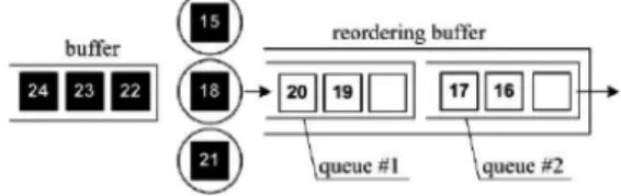
We consider the M/M/3/∞ queueing system (QS) with three servers, infinite capacity buffer, incoming Poisson flow of cus-tomers (of intensity λ) and exponential distribution of service time at each server (with parameter µ) and resequencing buffer (RB) of infinite capacity. Customer in reordering buffer may form two separate queues. The most convenient way to explain how queues are separated in resequencing buffer is giving an example. Con-sider a queueing system with three servers, infinite capacity main buffer and reordering buffer. Let the state of the system at some instant be as depicted in Fig. 1. In squares one can see customers’ sequential numbers. White (black) squares in Fig. 1 mean that customers with these sequential numbers have received (have not yet received) service. Here one can distinguish two queues: one which is formed by customers awaiting customer n. 18 (queue #1), another is formed by customers awaiting customer n. 15 (queue

(20)

#2). Three cases need to be considered.

1. If customer n. 21 is next to complete its service then it joins queue 1 and stays there until service of customer n. 18 is complete. Customer n. 22 joins idle server.

2. If customer n. 15 is next to complete its service then it goes through queue 1 without waiting and joins queue 2. Meanwhile customer n. 22 joins idle server. As there is no customer in the system with sequential number smaller than any sequential number in queue 2, then all customers from queue 2 leave the system. Resequencing buﬀer “sees”, that queue 2 is empty and moves its contents to queue 2. Now there are three options.

(a) if customer n. 18 is next to complete service, then it goes through queue 1 without waiting and joins queue 2. Customer n. 23 joins idle server. Again there is no customer in the system with sequential number smaller than any sequential number in queue 2. Thus all cus-tomers from queue 2 leave the system. Resequencing buﬀer becomes empty. Now if customer n. 21 is next to complete service, it leaves the system. If customer n. 22 is next to complete service, it goes through queue 1 without waiting and joins queue 2 where it waits for customer n. 21. Finally, if customer n. 23 is next to complete service, it joins queue 1 and does not proceed to queue 1 because it needs customer n. 22 to complete its service before both of them may join queue 2. (b) if customer n. 21 is next to complete service, then

it goes through queue 1 again without waiting, joins queue 2 and waits there with other customers for ser-vice completion of customer n. 18.

(c) if customer n. 22 is next to complete service, then cus-tomer n. 23 joins idle server, cuscus-tomer n. 22 joins queue 1 and stops there because “sees” gap between

(21)

2.1. Problem statement 15

its sequential number and largest sequential number in queue 2. It waits there for customer n. 21.

3. If customer n. 18 is the first to complete its service then it joins queue 1 and customer n. 22 joins idle server. Rese-quencing buﬀer “sees”, that there is no gap in the middle of sequence and moves the content of queue 1 to queue 2 (queue 1 becomes empty). Now there are again three options.

(a) if customer n. 15 is next to complete service, then it goes through queue 1 without waiting, joins queue 2 and immediately (because the sequence is complete) leaves the system with all other customers of queue 2. (b) if customer n. 21 is next to complete service, then it

goes through queue 1 again without waiting, joins other customers in queue 2 that wait for service completion of customer n. 15.

(c) if customer n. 22 is next to complete service, then it joins queue 1 and stops there, because “sees” gap be-tween its sequential number and the largest sequence number in queue 2. The operation of the system pro-ceeds along the line.

Figure 2.1 Scheme of the model.

Clearly, when the number of server is n there are (n-1) queues in resequencing buﬀer. The sum of customers in these (n-1) is the total number of customers in resequencing buﬀer.

(22)

The main contribution of this research are algorithm and proba-bility generating function of joint stationary probabilities of the number of customers in buﬀer, queue 1 and queue 2.

(23)

2.2. Model description and notation 17

2.2 Model description and notation

Customers upon entering the system obtain sequential number and join buﬀer. Without loss of generality we suppose that the sequence starts from 1 and coincides with the row of natural num-bers, i.e. the first customer upon entering the (empty) system re-ceives number 1, the second one number 2 and so on and so forth. Customers leave the system strictly in order of their arrival (i.e. in the sequence order). Thus after customer’s arrival it remains in the buﬀer for some time and then receives service when one of the servers becomes idle. If at the moment of its service completion there are no customers in the system or all other customers present at that moment in the queue and the rest two servers have greater sequential numbers, it leaves the system. Otherwise it occupies one place in the RB.

Customer from RB leaves it if and only if its sequential number is less than sequential numbers of all other customers present in system. Thus customers may leave RB in groups.

Let us call “1st _{level” customer the one which is in service and} was the last to enter server; “2nd _{level” customer is the one which} is in service and was the penultimate to enter server; finally, “3rd level” customer is the one which is in service and was the first to enter server. If the number of busy servers is 3, then customers that entered RB between “1st level” and “2ndlevel” customer form queue #1; customers which entered RB between “2nd _{level” and} “3rd_{level” customer form queue #2. If the number of busy servers} is 2, then customers which entered RB after “1st level” customer form queue #1; customers which entered RB between “1st _level” and “2nd _{level” customer form queue #2. When there is only one} busy server all customers in RB form queue #2.

The operation of the considered queueing system can be com-pletely described by a Markov process ζ(t) ={(ξ(t), η(t), υ(t)), t ≥ 0} with three components: ξ(t) - number of customers in buﬀer and server at time t, η(t) - number of customers in queue #1 of RB at time t, υ(t) - number of customers in queue #2 of RB at time t. In case ξ(t) = 0, the second and third component of ζ(t) are

(24)

omit-ted; in case ξ(t) = 1, the second is omitted. The state space of ζ(t) is χ = {0} ∪ {(1, i), i ≥ 0} ∪ {(n, i, j), n ≥ 2, i ≥ 0, j ≥ 0}. Hence-forth it is assumed that service and arrival processes are mutually independent and necessary and suﬃcient condition of stationarity

ρ

3 < 1, where ρ =

λ

µ, holds for the system.

Note that the total number of customers in servers and buﬀer of the considered QS with resequencing coincides with the total number of customers in M/M/3/∞ queue. Therefore, its station-ary distribution {pi, i≥ 0}, has the form:

p0 = ( ₂ ∑ i=0 ρi i! + ρ3 2!(3− ρ) )−1 , (2.2.1) pi = ρi i!p0, i = 1, 2, 3, (2.2.2) pi = ρi 3!3i−3p0 = ˜ρ i−3_p 3, ˜ρ = ρ 3, i≥ 4. (2.2.3) Provided that RB is empty when servers are idle, p0 is also

the probability, of the considered system with resequencing, to be empty.

Lets denote by pn;i,j, n ≥ 3, i ≥ 0, j ≥ 0, stationary probability of the fact that there are n customers in servers and buﬀer, i customers in queue #1 of RB, j customers in queue #2 of RB. By pn;i, n ≥ 3, i ≥ 0, denote stationary probability of the fact that there are n customers in servers and buﬀer and i customers in queue #1 of RB. Clearly pn;i =

∑

j≥0pn;i,j. Probabilities p2;i,j,

i≥ 0, j ≥ 0 and p2;i,, i≥ 0, are defined by analogy. Finally, let p1;i,

i ≥ 0, be stationary probability of the fact that there is only one busy server and i customers reside in queue #2 of RB. Note that distribution pn, n≥ 0, of the total number of customers in servers and buﬀer (which is defined by 2.2.1-2.2.3) can be expressed as follows: p1 = ∑ i≥0 p1;i, pn = ∑ i≥0 ∑ j≥0 pn;i,j, n≥ 2.

(25)

2.3. The equilibrium state distribution 19

2.3 The equilibrium state distribution

The system of equilibrium equations is composed by the following 12 equations:

(λ + 3µ) pn;0= λpn−1;0+ 2µpn+1, n≥ 3 (2.3.4) (λ + 3µ) pn;i= λpn−1;i+ µpn+1;i−1, n ≥ 3, i ≥ 1 (2.3.5) (λ + 2µ) p2;0 = λp1+ 2µp3, (2.3.6) (λ + 2µ) p2;i = µp3;i−1, i≥ 1 (2.3.7) (λ + µ) p1;0= λp0+ µp2;0, (2.3.8) (λ + µ) p1;i = µp2;i+ µ i−1 ∑ j=0 p2;i−j−1,j, i≥ 1 (2.3.9) (λ + 3µ) pn;0,0 = λpn−1;0,0+ µpn+1;0, n≥ 3 (2.3.10) (λ + 3µ) pn;0,j = λpn−1;0,j+µpn+1;j+µ j−1 ∑ k=0 pn+1;k,j−k−1, n ≥ 3, j ≥ 1 (2.3.11) (λ + 3µ) pn;i,j = λpn_−1;i,j+ µpn+1;i_−1,j, n≥ 3, i ≥ 1, j ≥ 0

(2.3.12) (λ + 2µ) p2;0,0 = λp1;0+ µp3;0, (2.3.13) (λ + 2µ) p2;0,j = λp1;j+ µp3;j+ µ j−1 ∑ k=0 p3;k,j−k−1, j ≥ 1 (2.3.14) (λ + 2µ) p2;i,j = µp3;i−1,j, i≥ 1, j ≥ 0. (2.3.15)

Now we describe them considering the transition diagram:

• (λ + 3µ) pn;0 = λpn−1;0 + 2µpn+1, n ≥ 3. Analyze the state (n; 0) and the rate in and the rate out of this state. State (n; 0) means that there are 3 busy servers, n customers between buﬀer and service, 0 customers in queue 1 and we don’t know how many customers there are in queue 2. Rate out of this state is λ + 3µ because system can exit it either

(26)

through arrival or through service. System can enter this state either: 1) by an arrival if all servers are busy, there are n− 1 customers between buﬀer and service and there are no customers in queue 1, 2) by service if all servers are busy, there are n + 1 customers in buﬀer and servers, and the 2nd or the 3th _{level customer could be served. Equating rate-in} and rate-out we get equation (2.3.4).

• (λ + 3µ) pn;i = λpn_−1;i+ µpn+1;i₋₁, n ≥ 3, i ≥ 1. Analyze the state (n; i) and the rate in and the rate out of this state. State (n; i) means that there are 3 busy servers, n customers between buffer and service, i customers in queue 1 and we don’t know how many customers there are in queue 2. Rate out of this state is λ + 3µ because system can exit it either through arrival or through service. System can enter this state either: 1) by an arrival if all servers are busy, there are n− 1 customers between buffer and service and there are i customers in queue 1, 2) by service if all servers are busy, there are n + 1 customers in buffer and servers, i− 1 customers in queue 1, and the 1st _{level customer is served.} Equating rate-in and rate-out we get equation (2.3.5). • (λ + 2µ) p2;0 = λp1+ 2µp3. Analyze the state (2; 0) and the

rate in and the rate out of this state. State (2; 0) means that there are 2 busy servers, 0 customers in queue 1 and we don’t know how many customers there are in queue 2. Rate out of this state is λ + 2µ because system can exit it either through arrival or through service. System can enter this state either: 1) by an arrival if only one server is busy, 2) by service if all servers are busy, there are 3 customers in service, and the 2nd_{or the 3}th_{level customer could be served.} Equating rate-in and rate-out we get equation (2.3.6). • (λ + 2µ) p2;i = µp3;i−1, i ≥ 1. Analyze the state (2; i) and

the rate in and the rate out of this state. State (2; i) means that there are 2 busy servers, i customers in queue 1 and we don’t know how many customers there are in queue 2.

(27)

Rate out of this state is λ + 2µ because system can exit it either through arrival or through service. System can enter this state: by service if all servers are busy, there are i− 1 customers in queue 1, and the 1st _{level customer is served.} Equating rate-in and rate-out we get equation (2.3.7). • (λ + µ) p1;0 = λp0+ µp2;0 . Analyze the state (1; 0) and the

rate in and the rate out of this state. State (1; 0) means that there is 1 busy server, 0 customers in queue 1 and we don’t know how many customers there are in queue 2. Rate out of this state is λ + µ because system can exit it either through arrival or through service. System can enter this state either: 1) by an arrival if servers are idle, 2) by service if 2 servers are busy, and the 3th _{level customer is served.} Equating rate-in and rate-out we get equation (2.3.8). • (λ + µ) p1;i = µp2;i + µ

i∑−1 j=0

p2;i−j−1,j, i ≥ 1. Analyze the

state (1; i) and the rate in and the rate out of this state. State (1; i) means that there is 1 busy server, i customers in queue 1 and we don’t know how many customers there are in queue 2. Rate out of this state is λ + µ because system can exit it either through arrival or through service. System can enter this state either: 1) by service if 2 servers are busy, there are i customers in queue 1 and the 3th _{level customer is} served, 2) by service if 2 servers are busy, there are i− j − 1 customers in queue 1 and j customers in queue 2, and the 2nd _{level customer is served. Equating rate-in and rate-out} we get equation (2.3.9).

• (λ + 3µ) pn;0,0 = λp_n−1;0,0 + µpn+1;0, n ≥ 3. Analyze the state (n; 0, 0) and the rate in and the rate out of this state. State (n; 0, 0) means that there are 3 busy servers, 0 cus-tomers in queue 1 and 0 cuscus-tomers in queue 2. Rate out of this state is λ + 3µ because system can exit it either through arrival or through service. System can enter this state ei-ther: 1) by an arrival if 3 servers are busy, there are n− 1

(28)

customers between buﬀer and servers, 0 customers in queue 1, 0 customers in queue 2, 2) by service if 3 servers are busy, there are n + 1 customers between buﬀer and service and 0 customers in queue 1, and the 3th _{level customer is served.} Equating rate-in and rate-out we get equation (2.3.10). • (λ + 3µ) pn;0,j = λpn_−1;0,j+ µpn+1;j+ µ

j∑−1 k=0

pn+1;k,j_−k−1, n ≥ 3, j ≥ 1. Analyze the state (n; 0, j) and the rate in and the rate out of this state. State (n; 0, j) means that there are 3 busy servers, 0 customers in queue 1 and j customers in queue 2. Rate out of this state is λ + 3µ because system can exit it either through arrival or through service. System can enter this state: 1) by an arrival if 3 servers are busy, there are n− 1 customers between buffer and servers, 0 customers in queue 1, j customers in queue 2, 2) by service if 3 servers are busy, there are n+1 customers between buffer and service and j customers in queue 1, and the 3th _{level customer is} served, 3) by service if 3 servers are busy, there are n + 1 customers between buffer and service, k customers in queue 1 and j − k − 1 customers in queue 2, and the 2nd _level customer is served. Equating rate-in and rate-out we get equation (2.3.11).

• (λ + 3µ) pn;i,j = λp_n−1;i,j+ µp_n+1;i−1,j, n ≥ 3, i ≥ 1, j ≥ 0. Analyze the state (n; i, j) and the rate in and the rate out of this state. State (n; i, j) means that there are 3 busy servers, i customers in queue 1 and j customers in queue 2. Rate out of this state is λ + 3µ because system can exit it either through arrival or through service. System can enter this state either: 1) by an arrival if 3 servers are busy, there are n− 1 customers between buﬀer and servers, i customers in queue 1, j customers in queue 2, 2) by service if 3 servers are busy, there are n + 1 customers between buﬀer and service, i− 1 customers in queue 1, j customers in queue 2 and the 1st _{level customer is served. Equating rate-in and rate-out} we get equation (2.3.12).

(29)

• (λ + 2µ) p2;0,0 = λp1;0 + µp3;0. Analyze the state (2; 0, 0)

and the rate in and the rate out of this state. State (2; 0, 0) means that there are 2 busy servers, 0 customers in queue 1 and 0 customers in queue 2. Rate out of this state is λ + 2µ because system can exit it either through arrival or through service. System can enter this state either: 1) by an arrival if 1 server is busy, there are no customers between buﬀer and servers, 2) by service if 3 servers are busy, there are no customers in queue 1, and the 3th _{level customer is served.} Equating rate-in and rate-out we get equation (2.3.13).

• (λ + 2µ) p2;0,j = λp1;j + µp3;j + µ

j∑−1 k=0

p3;k,j−k−1, j ≥ 1.

An-alyze the state (2; 0, j) and the rate in and the rate out of this state. State (2; 0, j) means that there are 2 busy servers, 0 customers in queue 1 and j customers in queue 2. Rate out of this state is λ + 2µ because system can exit it either through arrival or through service. System can enter this state either: 1) by an arrival if 1 server is busy, there are j customers in queue 1, 2) by service if 3 servers are busy, there are j customers in queue 1, and the 3th _{level customer} is served, 3) by service if 3 servers are busy, there are k cus-tomers in queue 1 and j−k−1 customers in queue 2, and the 2nd _{level customer is served. Equating rate-in and rate-out} we get equation (2.3.14).

• (λ + 2µ) p2;i,j = µp3;i−1,j, i ≥ 1, j ≥ 0. Analyze the state

(2; i, j) and the rate in and the rate out of this state. State (2; i, j) means that there are 2 busy servers, i customers in queue 1 and j customers in queue 2. Rate out of this state is λ + 2µ because system can exit it either through arrival or through service. System can enter this state either: 1) by service if all servers are busy, there are i− 1 customers in queue 1, j customers in queue 2 and the 1st _{level customer} is served. Equating rate-in and rate-out we get equation (2.3.15).

(30)

The analysis of steady-state equations resulted in the develop-ment of simple algorithm for step-by-step computation of station-ary joint probabilities pn;i,j, n≥ 2, i ≥ 0, j ≥ 0 and pn;i, n≥ 1, i ≥ 0.

The algorithm is the following: Inizialize λ, µ;

for n ≥ 0 do:

calculate pn from equation (2.2.1), (2.2.2), (2.2.3); end for

calculate p2;0 from equation (2.3.6);

for n ≥ 3 do:

calculate pn;0 from equation (2.3.4); end for

for i≥ 1 do:

calculate p2;i from equation (2.3.7);

for n≥ 3 do:

calculate pn;i from equation (2.3.5); end for

end for

calculate p1;0 from equation (2.3.8);

calculate p2;0,0 from equation (2.3.13);

for n ≥ 3 do:

calculate pn;0,0 from equation (2.3.10); end for

for i≥ 1 do:

calculate p2;i,0 from equation (2.3.15);

for n≥ 3 do:

calculate pn;i,0 from equation (2.3.12); end for

end for for i≥ 2 do:

calculate p1;i from equation (2.3.9);

calculate p2;0,i from equation (2.3.14);

for n≥ 3 do:

(31)

end for for j ≥ 1 do:

calculate p2;j,i from equation (2.3.15);

for m≥ 3 do:

calculate pm;i,j from equation (2.3.12); end for

end for end for

For practical purposes it may be sometimes sufficient to know either only πn;i n ≥ 1, i ≥ 0 - stationary probabilities of the fact that total number of customers in servers and in buffer is n and total number of customers in RB (sum of queue #1 and queue #2) is i, or only πi, i ≥ 0 - stationary probabilities of the fact that there are n customers in total in the whole system (including buffer, servers, RB). These quantities can be calculated from joint probability distribution as follows:

π1;i = p1;i, i≥ 0, π2;i =

i ∑ j=0 p2;j,i−j, i≥ 0, πn;i= i ∑ j=0 pn;j,i−j, n ≥ 3, i ≥ 0, π0 = p0, π1 = π1;0, π2 = π1;1+ π2;0, πi = π1;i−1+ π2;i−2+ i ∑ j=3 πj;i−j, i≥ 3.

(32)

2.4 Probability generating functions

Though the calculation of probabilities pn;i,j, n ≥ 2, i ≥ 0, j ≥ 0 and pn;i, n ≥ 1, j ≥ 0 is just a matter of computational eﬀort due to obtained above algorithm, performance characteristics (e.g. moments and/or correlation of queue lengths in RB) are not so straightforward to obtain. Below we show that in the considered case one can obtain expressions for probability generating func-tions (PGF) that ease the computation of various performance characteristics. Let us introduce the following PGF:

pn(z) = ∞ ∑ i=0 zipn;i, 0≤ z ≤ 1, n ≥ 1, pn(z1, z2) = ∞ ∑ i1=0 ∞ ∑ i2=0 zi1 1 z i2 2 pn;i1,i2, 0≤ z1 ≤ 1, 0 ≤ z2 ≤ 1, n ≥ 2, P (u, z) = ∞ ∑ n=3 un−3pn(z), 0≤ u ≤ 1, P (u, z1, z2) = ∞ ∑ n=3 un−3pn(z1, z2), 0≤ u ≤ 1.

If one puts z1 = z2 = z in P (u, z1, z2), then function P (u, z, z) is

the double PGF of the total number of customers in buﬀer and servers and total number of customers in RB when all three servers are busy. By analogy pn(z, z), n≥ 2, is the PGF of the total num-ber of customers: total numnum-ber of customers in RB and probability of total n customers in servers and buﬀer. In the following we will make use of PGF P (u) = ∑∞

n=3

un−3pn,|u| ≤ 1 which, with respect to (2.2.1)-(2.2.3), equals P (u) = p3

1−˜ρu.

Now we will successively obtain relations for PGF defined above. Start with the following equations:

(33)

2.4. Probability generating functions 27

pn;i(λ + 3µ) = pn−1;iλ + pn+1;i−1µ, n≥ 3, i ≥ 1. (2.4.17) We multiply for zi _{and sum on i only the equation (4.3.1) because} of the equation (2.4.16) does not depend on i :

∞ ∑ i=1 zipn;i(λ + 3µ) = ∞ ∑ i=1 zipn−1;iλ + ∞ ∑ i=1 zipn+1;i−1µ n≥ 3, i ≥ 1 from which we obtain:

(λ + 3µ) [pn(z)− pn;0] = λ [pn−1(z)− pn−1;0] + µzpn+1(z) (2.4.18) Here we sum (2.4.16) with (4.3.5) in order to find pn(z) :

pn(z) = 1

λ + 3µ[2µpn+1+ λpn−1(z) + µzpn+1(z)] n ≥ 3 (2.4.19) Then we analize the following equations:

p2;0(λ + 2µ) = p1λ + p32µ (2.4.20)

p2;i(λ + 2µ) = p3;i−1µ i≥ 1 (2.4.21)

Multiplying for zi and summing on i only the equation (2.4.21), because of the equation (2.4.20) does not depend on i, we obtain:

∞ ∑ i=1 zip2;i(λ + 2µ) = ∞ ∑ i=1 zip3;i−1µ i≥ 1 (λ + 2µ) [ _∞ ∑ i=0 zip2;i− p2;0 ] = µz ∞ ∑ t=0 ztp3;t (λ + 2µ) [p2(z)− p2;0] = µzp3(z) (2.4.22)

Now we sum (2.4.20) with (2.4.22) in order to find p2(z) :

p2(z) =

1

λ + 2µ[λp1+ 2µp3+ µzp3(z)] (2.4.23) We analize the following equations:

(34)

p1;i(λ + µ) = p2;iµ +

i−1 ∑

j=0

p2;i−j−1,jµ i≥ 1 (2.4.25)

We multiply for zi and sum on i only the equation (2.4.25) because of the equation (2.4.24) does not depend on i :

∞ ∑ i=1 zip1;i(λ + µ) = ∞ ∑ i=1 zip2;iµ + ∞ ∑ i=1 zi i−1 ∑ j=0 p2;i−j−1,jµ i≥ 1 (λ+µ) [ _∞ ∑ i=0 zip1;i− p1;0 ] = µ [ _∞ ∑ i=0 zip2;i− p2;0 ] + ∞ ∑ i=1 zi i−1 ∑ j=0 p2;i−j−1,jµ (λ + µ) [p1(z)− p1;0] = µ [p2(z)− p2;0] + ∞ ∑ i=1 i−1 ∑ j=0 zip2;i−j−1,jµ (2.4.26) In order to find p1(z) we sum (2.4.24) with (2.4.26):

p1(z) = 1 λ + µ [ p0λ + µp2(z) + µz ∞ ∑ t=0 t ∑ j=0 ztp2;t−j,j ] (2.4.27)

and we observe that for t− j = k: ∞ ∑ k+j=0 k+j ∑ j=0 zk+jp2;k,j = ∞ ∑ k+j=0 ∞ ∑ j=0 zk+jp2;k,j = p2(z, z) so p1(z) = 1 λ + µ [p0λ + µp2(z) + µzp2(z, z)] (2.4.28) The next step is to analize the following equations:

pn;0,0(λ + 3µ) = pn_−1;0,0λ + pn+1;0 n≥ 3 (2.4.29) pn;0,j(λ+3µ) = pn−1;0,jλ+pn+1;jµ+ j−1 ∑ k=0 pn+1;k,j−k−1µ n≥ 3, j ≥ 1 (2.4.30)

(35)

pn;i,j(λ + 3µ) = pn−1;i,jλ + pn+1;i−1,jµ n ≥ 3, i ≥ 1, j ≥ 0 (2.4.31) We multiply for z₂j and sum on j the equation (2.4.30), then we multiply for zi

1 and z

j

2 and sum on i and on j the equation (2.4.31),

while the equation (2.4.29) does depend neither on i or on j : ∞ ∑ j=1 z₂jpn;0,j(λ + 3µ) = ∞ ∑ j=1 z₂jpn−1;0,jλ + ∞ ∑ j=1 z₂jpn+1;jµ+ + ∞ ∑ j=1 z₂j j−1 ∑ k=0 pn+1;k,j_−k−1µ n ≥ 3, j ≥ 1 and after manipulations:

(λ + 3µ) [ _∞ ∑ j=0 z₂jpn;0,j − pn;0,0 ] = λ [ _∞ ∑ j=0 zj₂pn−1;0,j− pn−1;0,0 ] + (2.4.32) +µ [pn+1(z2)− pn+1;0] + µz2 [ _∞ ∑ t=0 t ∑ k=0 z₂tpn+1;k,t−k ]

Here we study the equation (2.4.31): ∞ ∑ j=0 z₂j ∞ ∑ i=1 z₁ipn;i,j(λ + 3µ) = ∞ ∑ j=0 zj₂ ∞ ∑ i=1 z₁ipn−1;i,jλ+ + ∞ ∑ j=0 z₂j ∞ ∑ i=1 z₁ipn+1;i−1,jµ n ≥ 3, i ≥ 1, j ≥ 0

introducing the term for i = 0 and after appropriate manipula-tions, we find: (λ+3µ) [ pn(z1, z2)− ∞ ∑ j=0 z₂jpn;0,j ] = λ [ pn−1(z1, z2)− ∞ ∑ j=0 z₂jpn−1;0,j ] + (2.4.33) +µz1pn+1(z1, z2)

(36)

In order to find pn(z1, z2) we sum (2.4.29), (2.4.32) and (2.4.33): pn;0,0(λ + 3µ) + (λ + 3µ) [ _∞ ∑ j=0 zj₂pn;0,j− pn;0,0 ] + (λ + 3µ) [ pn(z1, z2)− ∞ ∑ j=0 z₂jpn;0,j ] = pn_−1;0,0λ + pn+1;0+ +λ [ _∞ ∑ j=0 zj₂pn−1;0,j− pn−1;0,0 ] + µ [pn+1(z2)− pn+1;0] + +µz2 [ _∞ ∑ t=0 t ∑ k=0 zt₂pn+1;k,t−k ] + λ [ pn−1(z1, z2)− ∞ ∑ j=0 z₂jpn−1;0,j ] + +µz1pn+1(z1, z2)

observing that t = k + s we obtain: ∞ ∑ k+s=0 ∞ ∑ k=0 z₂k+spn+1;k,s= p2(z2, z2) so pn(z1, z2) = 1 (λ + 3µ)[µpn+1(z2) + z2µp2(z2, z2)+ +λpn−1(z1, z2) + µz1pn+1(z1, z2)]

Here we analize the following equations:

p2;0,0(λ + 2µ) = p1;0λ + p3;0µ (2.4.34) p2;0,j(λ + 2µ) = p1;j+ p3;jµ + j−1 ∑ k=0 p3;k,j−k−1µ j ≥ 1 (2.4.35)

(37)

p2;i,j(λ + 2µ) = p3;i−1,jµ i≥ 1, j ≥ 0 (2.4.36)

Now we multiply for z₂j and sum on j the equation (2.4.35), then we multiply for zi

1 and z

j

2 and sum on i and on j the equation

(2.4.36), while the equation (2.4.34) does depend neither on i or on j : ∞ ∑ j=1 zj₂p2;0,j(λ+2µ) = λ ∞ ∑ j=1 z₂jp1;j+ ∞ ∑ j=1 z₂jp3;jµ+ ∞ ∑ j=1 z₂j j−1 ∑ k=0 p3;k,j−k−1µ j ≥ 1 (λ+2µ) [ _∞ ∑ j=0 z₂jp2;0,j− p2;0,0 ] = λp1(z2)−λp1;0+µ [p3(z2)− p3;0] + (2.4.37) +µz ∞ ∑ t=0 z₂t t ∑ k=0 p3;k,t−k ∞ ∑ j=0 z₂j ∞ ∑ i=1 z₁ip2;i,j(λ + 2µ) = ∞ ∑ j=0 z₂j ∞ ∑ i=1 z₁ip3;i−1,jµ i≥ 1, j ≥ 0

as in the previous case, we introduce the term for i = 0 and after appropriate substitutions we find:

(λ + 2µ) [ p2(z1, z2)− ∞ ∑ j=0 zj₂p2;0,j ] = µz1p3(z1, z2) (2.4.38)

In the next step we sum (2.4.34), (2.4.37) and (2.4.38) in order to find p2(z1, z2): p2;0,0(λ + 2µ) + (λ + 2µ) [ _∞ ∑ j=0 zj₂p2;0,j− p2;0,0 ] + (λ + 2µ) [ p2(z1, z2)− ∞ ∑ j=0 zj₂p2;0,j ] = p1;0λ + p3;0µ + λp1(z2)− λp1;0+

(38)

+µ [p3(z2)− p3;0] + µz ∞ ∑ t=0 z₂t t ∑ k=0 p3;k,t−k + µz1p3(z1, z2)

we observe that for t = a + k we get: ∞ ∑ a+k=0 z₂a+k ∞ ∑ k=0 p3;k,a= p3(z2, z2) so p2(z1, z2) = 1 λ + 2µ[λp1(z2) + µp3(z2) + µz2p3(z2, z2)+ (2.4.39) +µz1p3(z1, z2)] We find P (u, z) : ∞ ∑ n=3 un−3(λ + 3µ)pn(z) = ∞ ∑ n=3 un−3[2µpn+1+ λpn−1(z) + µzpn+1(z)] (λ + 3µ) ∞ ∑ n=3 un−3pn(z) = ∞ ∑ n=3 [ un−32µpn+1+ un−3λpn−1(z)+ +un−3µzpn+1(z) ] (λ + 3µ)P (u, z) = ∞ ∑ n=3 un−32µpn+1+ + ∞ ∑ n=3 un−3λpn−1(z) + ∞ ∑ n=3 un−3µzpn+1(z)

Thanks to the notations introduced at the beginning of this chap-ter, we can write a better expression using P (u), P (u, z) :

(λ + 3µ)P (u, z) = 2µ u [ _∞ ∑ n=3 un−3pn− p3 ] + λ ∞ ∑ n=3 un−3pn−1(z)+ +µz ∞ ∑ n=3 un−3pn+1(z)

(39)

2.4. Probability generating functions 33 (λ + 3µ)P (u, z) = 2µ u [P (u)− p3] + λ ∞ ∑ n=3 un−3pn−1(z)+ +µz ∞ ∑ n=3 un−3pn+1(z) (λ + 3µ)P (u, z) = 2µ u [P (u)− p3] + λ [ u ∞ ∑ n=3 un−3pn(z) + p2(z) ] + +µz ∞ ∑ n=3 un−3pn+1(z) (λ + 3µ)P (u, z) = 2µ

u [P (u)− p3] + λ [uP (u, z) + p2(z)] + +µz u [ _∞ ∑ n=3 un−3pn(z)− p3(z) ] (λ + 3µ)P (u, z) = 2µ

u [P (u)− p3] + λ [uP (u, z) + p2(z)] + +µz

u[P (u, z)− p3(z)]

u(λ + 3µ)P (u, z) = 2µ [P (u)− p3] + λu2P (u, z)+

λup2(z) + µzP (u, z)− µzp3(z)

Finally we obtain:

P (u, z) = µzp3(z)− λµp2(z)− 2µ [P (u) − p3]

λu2_{+ µz}− u(λ + 3µ) (2.4.40)

The next step is to find P (u, z1, z2) :

(λ + 3µ) ∞ ∑ n=3 un−3pn(z1, z2) = ∞ ∑ n=3 un−3[µpn+1(z2)+ +z2µpn+1(z2, z2) + λpn−1(z1, z2) + µz1pn+1(z1, z2)] (λ + 3µ)P (u, z1, z2) = λ ∞ ∑ n=3 un−3pn−1(z1, z2) + ∞ ∑ n=3 un−3µpn+1(z2)+

(40)

+ ∞ ∑ n=3 un−3µz2pn+1(z2, z2) + ∞ ∑ n=3 un−3µz1pn+1(z1, z2) (λ + 3µ)P (u, z1, z2) = λ [ u ∞ ∑ n=3 un−3pn(z1, z2) + p2(z1, z2) ] + +µ u [ _∞ ∑ n=3 un−3pn(z2)− p3(z2) ] +µ uz2 [ _∞ ∑ n=3 un−3pn(z2, z2)− p3(z2, z2) ] + +µ uz1 [ _∞ ∑ n=3 un−3pn(z1, z2)− p3(z1, z2) ]

(λ + 3µ)P (u, z1, z2) = λ [uP (u, z1, z2) + p2(z1, z2)] +

µ u[P (u, z2) + −p3(z2)]+ µ uz2[P (u, z2, z2)− p3(z2, z2)]+ µ uz1[P (u, z1, z2)− p3(z1, z2)] P (u, z1, z2) = 1 λu2_{+ µz} 1− (λ + 3µ)u [−λup2(z1, z2)+ (2.4.41) −µ [P (u, z2)− p3(z2)]− µz2[P (u, z2, z2)− p3(z2, z2)] + µz1p3(z1, z2)]

Assuming z1 = z2 = z we find P (u, z, z) and p2(z, z) :

P (u, z, z) = 1

λu2_{+ 2µz}− (λ + 3µ)u[−λup2(z, z)+ (2.4.42)

−µ [P (u, z) − p3(z)] + 2µzp3(z, z)]

p2(z, z) =

1

(λ + 2µ)[λp1(z) + µp3(z) + 2µzp3(z, z)] (2.4.43) In order to find solution of the denominator P (u, z, z) we consider:

fm(u, z) = λu2 + mµz− (λ + 3µ)u m = 1, 2 and study:

(41)

2.4. Probability generating functions 35 from which um = λ + 3µ−√(λ + 3µ)2− 4mλµz 2λ and ˆ um = λ + 3µ +√(λ + 3µ)2− 4mλµz 2λ = λ + 3µ λ − um If z = 0 : um = λ + 3µ− √ (λ + 3µ)2 2λ = 0 If z = 1 : ˆ um = λ + 3µ + √ (λ + 3µ)2− 4mλµ 2λ = 1

Now we rewrite P (u, z) and P (u, z, z) :

P (u, z) = µzp3(z)− λµp2(z)− 2µ [P (u) − p3] f1(u, z) (2.4.44) P (u, z, z) = 1 f2(u, z) [−λup2(z, z)− (2.4.45) µ [P (u, z)− p3(z)] + 2µzp3(z, z)]

Denominator in (2.4.44) and (2.4.45) is zero at points (u1, z) =

(u1(z), z) and (u2, z) = (u2(z), z). Since PGF P (u, z, z) is analytic

function in the domain 0≤ z ≤ 1 then numerator must be zero at these points too. This leads to the following equations:

µzp3(z)− λu1p2(z)− 2µ [P (u1)− p3] = 0 (2.4.46)

2µzp3(z, z)− λu2p2(z, z)− µ [P (u2, z)− p3(z)] = 0 (2.4.47)

Firstly we find PGF P (u, z). Solution of equations (2.4.23) and (2.4.46):

{

(λ + 2µ)p2(z)− µzp3(z) = λp1+ 2µp3

(42)

{ (λ + 2µ)p2(z)− [2µ [P (u1)− p3] + λu1p2(z)] = λp1+ 2µp3 p3(z) = _µz1 [2µ [P (u1)− p3] + λu1p2(z)] { p2(z) = _2µ+λ1_−λu₁ [λp1− 2µP (u1)] p3(z) = _µz1 [2µ [P (u1)− p3] + λu1p2(z)]

Now we substitute p2(z) and p3(z) in P (u, z):

P (u, z) = 1 f1(u, z) [ µz 1 µz [λu1p2(z) + 2µ [P (u1)− p3]] + − (λµ)λp1+ 2µP (u1) λ− λu1+ 2µ − 2µ [P (u) − p3] ] = 1 f1(u, z) [ λu1p2(z) + 2µ [P (u1)− p3]− (λµ) λp1+ 2µP (u1) λ− λu1 + 2µ + −2µ [P (u) − p3]] = 1 (u− u1) (u− û1) [ λu1 λp1+ 2µP (u1) λ− λu1+ 2µ + 2µ [P (u1)− P (u)] + −λuλp1 + 2µP (u1) λ− λu1+ 2µ ] = 1 (u− u1) (u− û1) [ p2(z)(λu1 − λu) + 2µ ( p3 1− ˜ρu1 − p3 1− ˜ρu )] = 1 (u− u1) (u− û1) [p2(z)(λu1− λu)+ +2µ ( p4 ˜ ρ(1− ˜ρu1) − p4 ˜ ρ(1− ˜ρu) )] = 1 (u− u1) (u− û1) [ λp2(z)(u1− u) + 2µ p4ρ(u˜ 1− u) ˜ ρ(1− ˜ρu)(1 − ˜ρu1) ] substitute p2(z): = 1 (u− û1) [ −λp2(z)− 2µp4 (1− ˜ρu)(1 − ˜ρu1) ] = 1 (u− û1) [ −λλp1+ 2µP (u1) λ− λu1 + 2µ − 2µp4 (1− ˜ρu)(1 − ˜ρu1) ]

(43)

2.4. Probability generating functions 37 substitute P (u1): = 1 (u− ˆu1) [ −λλp1+ 2µ p3 1−˜ρu1 λ− λu1+ 2µ − 2µp4 (1− ˜ρu)(1 − ˜ρu1) ] = λ (ˆu1− u) (1 − ˜ρu1) [ [λ + 2µ]p2;0− λp1ρu˜ 1 (λ− λu1+ 2µ) + 2µp4 (1− ˜ρu) ] (2.4.48) Now we find the expression for P (u, z, z). Solving system of equa-tions (2.4.28), (2.4.43) and (2.4.47), one obtains the following ex-pression for PGFs p1(z), p2(z, z) and p3(z, z):

p1(z) = 1 λ + µ[λp0+ µp2(z) + µzp2(z, z)] p3(z, z) = 1 2µz [λu2p2(z, z) + µ [P (u2, z)− p3(z)]] p2(z, z) = 1 λ− λu2+ 2µ−_λ+µλµz [ 1 λ + µ[λp0+ µp2(z)] + µP (u2, z) ]

If one substitutes expression for p1(z), p2(z, z) and p3(z, z) into

(2.4.45) then, after collecting the common terms, one finds P (u, z, z). The last PGF to find is P (u, z1, z2). Denominator in (2.4.41) is

zero at point (u1(z1), z1). Since PGF P (u, z1, z2) is an analytic

function in the domain 0 ≤ z1 ≤ 1, 0 ≤ z2 ≤ 1 then numerator

must vanish at this point. Hence it holds:

−λu1(z1)p2(z1, z2)− µ [P (u1(z1), z2)− p3(z2)] + (2.4.49)

−µz2[P (u1(z1), z2, z2)− p3(z2, z2)] + µz1p3(z1, z2) = 0.

From relation (2.4.39) it follows that:

µz1p3(z1, z2) = (λ+2µ)p2(z1, z2)−λp1(z2)−µp3(z2)−µz2p3(z2, z2).

Substitution of µz1p3(z1, z2) into (2.4.49), leads to the expression

for p2(z1, z2):

p2(z1, z2) =

1

[λ + 2µ− λu1(z1)]

(44)

+µz2P (u1(z1), z2, z2)]

Thus we have obtained all the unknown quantities in PGF P (u1, z1, z2) and it is determined completely.

(45)

2.5. Numerical results 39

2.5 Numerical results

There are several quantities related to the number of customers in the system that may be of interest. They are mean and variance of the number of customers in queue 1 and queue 2, correlation between queue size in buﬀer and queue 1, between queue size in buﬀer and queue 2 and between queue 1 and queue 2. These quan-tities are calculated considering λ = 2.5, µ = 1 and n = 100. In the Figure 2.2 the upper, the middle and the lower line represents respectively the mean number of customers in RB, queue 2 of RB and queue 1 of RB:

Figure 2.2 Mean number of customers.

We observe that the mean number of customers in RB is the sum of the mean number of customers in queue 1 of RB and queue 2 in RB. In the Figure 2.3 the upper, the middle and the lower line represents respectively the variance of the number of customers in RB, queue 2 of RB and queue 1 of RB.

We observe that the variance of the number of customers in RB is almost the sum of the variance of the number of customers in queue 1 of RB and queue 2 of RB, and this is strange because it is well known that V ar(X + Y ) = V ar(X) + V ar(Y ) + Cov(X, Y ),

(46)

Figure 2.3 Variance of the number of customers.

where X is the number of customers in queue 1 of RB and Y is the number of customers in queue 2 of RB, so the Cov(X, Y )∼ 0. In fact if we observe the Figure 2.4 where the upper, the middle and the lower line represents respectively the correlation between buﬀer and queue 1 of RB, between buﬀer and queue 2 of RB, between queue 1 and queue 2 of RB, we notice that the correla-tion between queue 1 and queue 2 of RB is almost equal to zero, so the number of customers in queue 1 of RB and the number of customers in queue 2 of RB are almost uncorrelated, so the V ar(X + Y ) is almost equal to V ar(X) + V ar(Y ).

(47)

2.5. Numerical results 41

(48)

(49)

Chapter 3 N-server queueing system

with poisson input and

exponential service times

3.1 Problem statement

We consider a queueing system with 3 < N <∞ servers, infinite capacity buffer, incoming Poisson flow of customers (of intensity λ), exponential distribution of service time in each server (with parameter µ) and resequencing buffer (RB) of infinite capacity. Customers upon entering the system obtain sequential number and join buffer. Without loss of generality we suppose that the sequence starts from 1 and coincides with the row of natural num-bers, i.e. the first customer upon entering the (empty) system re-ceives number 1, the second one number 2 and so on and so forth. Customers leave the system strictly in order of their arrival. Thus after customer’s arrival it remains in the buffer for some time and then receives service when one of the servers becomes idle. If at the moment of its service completion there are no customers in the system or all other customers present at that moment in the queue and in all other servers have greater sequential numbers, it leaves the system. Otherwise it occupies one place in the RB. Customer from RB leaves it if and only if its sequential number

(50)

is less than sequential number of all other customers present in system i.e. customers may leave RB in groups.

(51)

3.2. Model description and notation 45

3.2 Model description and notation

As it was mentioned in the previous section customers awaiting in RB may form separate (virtual) queues. In order to explain this let us introduce the following notation. If there are n, n = 1, .., N busy servers, we call “1st_{level” customer the last one (among those} n in servers) which joined the system; we call “2nd _{level” customer} the penultimate customer which joined the system (among those n in servers); “3rd _{level” customer is the one which joined the} system before the penultimate customer etc. The customer which was the first (among those n in servers) to join the system is “nth_{level” customer. If at some instant all servers are busy i.e.} n = N , then customers which joined RB between “1st _{level” and} “2nd level” customer form queue 1; customers which joined RB between “2nd _{level” and “3}rd _{level” customer form queue 2 etc.} Clearly, customers which joined RB between “(n− 1)th _{level” and} “nth level” customer form queue (N-1). Notice that if at some instant n < N , then customers which joined RB after “1st _level” customer form queue 1; customers which joined RB between “1st level” and “2nd level” customer form queue 2 etc. The operation of the considered queueing system can be completely described by Markov process ζ(t) = {(ξ(t), η1(t), η2(t), ..., ηN−1(t)), t ≥ 0} where ξ(t) is the number of customers in buﬀer and all servers at time t, ηi(t) is the number of customers in queue #i of RB at time t. In case ξ(t) = 0, the all but first component of ζ(t) are omitted; in case ξ(t) = n, n = 1, ..., N − 2, the last N − 1 − n components are omitted. The state space of ζ(t) is:

χ ={0} ∪ {(1, i1), i1 ≥ 0} ∪ {(2, i1, i2), i1 ≥ 0, i2 ≥ 0} ∪ ...

∪{(2, i1, i2, ..., iN−1), n≥ N − 1, i1, i2, ..., iN−1 ≥ 0}.

It is assumed that service and arrival processes are mutually in-dependent and necessary and suﬃcient condition of stationarity ˜

ρ = _Nρ < 1, where ρ = λ_µ holds for the system. Indeed one can notice that the total number of customers in buﬀer and servers of the considered QS with resequencing coincides with the total num-ber of customers in M/M/∞/∞ queue. Therefore, its stationary