Introduction i
1 Aeroportual’s Domain 1
1.1 ATC - Basic Concept . . . 1
1.2 The airport in the international context . . . 3
1.3 The phases of departure and landing in the life cycle of a flight . . 4
1.3.1 Pre-flight, Taxi and Take-off . . . 5
1.3.2 Climb . . . 6
1.3.3 En-Route . . . 6
1.3.4 Descent and approach . . . 7
1.3.5 Taxi and Arrival . . . 7
2 Problem Statement and State of the Art 9 2.1 Departure Flight Scheduling . . . 9
2.2 Aeroportual Safety Rules and Goals . . . 11
2.3 Minimum separation between aircraft . . . 13
2.4 Departures routes . . . 14
2.5 Calculated Take-off Time . . . 14
2.6 State of the Art . . . 15
2.7 Single Stage Methodology . . . 16
2.7.1 Multi-objective modeling . . . 19
2.7.2 Planning: solution . . . 20
2.8 Double Stage Methodology . . . 21
2.8.1 First stage . . . 22
CONTENTS
2.8.3 Objective Function . . . 23
2.8.4 Sequences’s Classes . . . 23
2.8.5 First Stage Output . . . 23
2.8.6 Second Stage . . . 24
2.8.7 Objective Function . . . 26
2.8.8 Approach based on CSP . . . 27
2.9 Approach based on queueing theory . . . 32
2.9.1 Application context . . . 32
2.9.2 Heuristics for the assignment of path . . . 33
2.9.3 Departure Scheduling Algorithms . . . 34
2.9.4 Formal mathematical model . . . 35
3 Two Stage Algorithm: Formal Model 38 3.1 Introduction . . . 38
3.2 Two Stage Algorithm . . . 39
3.3 First stage . . . 44
3.4 Formal model for the first stage . . . 46
3.5 First Stage Mathematical Model . . . 48
3.6 Heuristic for Mixing Arrivals and Departures . . . 50
3.7 Second Stage Mathematical Model . . . 51
3.8 Second Stage Mathematical Model . . . 56
3.9 Freezed Flight . . . 57
3.10 The multi-runway procedure . . . 58
3.10.1 Configuration Procedure . . . 59
3.10.2 Sequencing Procedure . . . 60
3.10.3 Capacity Control . . . 61
4 Simulations and Results 63 4.1 Introduction . . . 63 4.2 Scenario #1 . . . 64 4.3 Scenario #2 . . . 68 4.4 Scenario #3 . . . 70 4.5 Scenario #4 . . . 72 4.5.1 Setup of scenario . . . 73
List of Figures
1.1 Italian FIR . . . 3 1.2 Flight Phases . . . 4 1.3 Flight Phases . . . 5 1.4 Climb . . . 6 1.5 En-Route . . . 71.6 Descent and approach . . . 7
1.7 Taxi and Arrival . . . 8
2.1 Vortex behind the aircraft . . . 13
2.2 An example of a two-dimensional, non-convex, disjoint search space T(C) (white area) 18 2.3 The Layout of London Heathrow Airport . . . 32
2.4 An example of holding point network structure . . . 33
3.1 Flowchart of algorithm Two Stage . . . 43
3.2 Separation times between weight class . . . 45
3.3 Example of reduction to ATSP problem . . . 48
3.4 Second Stage graph . . . 52
3.5 Input graph for the Second Stage Algorithm . . . 54
3.6 Output graph for the Second Stage Algorithm . . . 55
3.7 Two stages algorithm dataflow . . . 59
1 DMAN gui . . . 82
Punctuality is a key element in aviation: the delays are a “failure” promise for the passenger and it carry a heavy cost and difficulty to the entire sector. The development of air transport in recent decades has occurred within a com-plex framework characterized by profound changes in technical, managerial and organizational likely to provide an adequate response to a growing demand. These changes were originated both from the aviation industry pressures and the need to liberalize a sector strong growth. After a collapse in air traffic growth due to the global economic crisis of recent years, a constant increase in demand has been, and forecasts for the coming years are positive.
To this steady increase in air traffic demand has not been matched by an adequate growth of the capacity of the system infrastructural networks. The main effect of this phenomenon are situations of congestion that creates delay on the ground and at departure and arrival queues, and causing difficulties to passengers and huge losses to airlines.
The capacity may be increased by providing the airport with a sufficient num-ber of runways and parking bay; it is clear that if these structures are lacking or insufficient the infrastructural capacity on the ground has negative effects on the airspace’s capacity. In the short term, the best we can get from the system is to limit the impact of delays, caused by congestion, controlling the air traffic flow in order to match the demand with the available capacity. This activity is defined: Air Traffic Flow Management (or ATFM).
In Europe, a continent with many nations and airspaces. the air traffic and air flow control is a complex problem. The coordination and centralization task was entrusted to the ”Central Flow Management Unit” (or CFMU), that control the air
Introduction
traffic flow for 36 nations of the European Civil Aviation Conference1. The activity of flight assistance in Italy is provided by ENAV Spa that in addition to providing air navigation services and the development of new technology systems, it has as main objective to increase the ATC (Air Traffic Control) capacity, obviously treating the safety as a key component of the system.
Research on air traffic management began in the the late 80s, and they have mainly focused on models of optimization for the allocation of the delay to the ground. In this thesis In this work we introduce a mathematical model to im-prove the aircraft departures planning system. The objective is to maximize the airport performances, minimize delays in the runway operations and to support the air controller work. The followed approach is based on the combination of a one runway two stages algorithm with a multi-runway procedure to find the better departures scheduling. By means of the two stages algorithm, a complex problem dealing with multi-objective functions is split into two inter-connected one dimen-sional problems. In the first stage the aim is to minimize the throughput, defined as the number of aircraft in the time unit, subject to Wake Vortex Separations constraint. An ad-hoc control heuristic method is used to mix the pre-fixed land-ing arrivals slots with the departure slots outgoland-ing from the first stage. In the second stage the class sequence, generated by the first one, is computed in order to minimize the delays between the actual and estimated take-off time of each departing aircraft, subject to fixed CTOTs and ETOTs, and considering some possible departing priority. Successively a multi-runway procedure is introduced, consisting of an heuristic methodology, which uses the two stage algorithm, to locate as better as possible the aircraft on each available runway. The result is the better feasible take-off sequence in a referred time window. Some simulations on typical flight strips from Milano Malpensa airport in Italy, having two runways, are shown.
This paper is organized as follows:
• in the first chapter we introduce the main players of the airport system and
1
ECAC is an intergovernmental organization which was established by the International Civil Aviation Organization (ICAO) and the Council of Europe. It promotes the continued development of a safe, efficient and sustainable European air transport system. In doing so, it seeks harmonies civil aviation policies and practices amongst its Member States and promote understanding on policy matters between its Member States and other parts of the world
its terminology in use.
• in the second chapter we discuss some of the works presented in the literature concerning the problem of departure scheduling. In particular, we focus on the work of Anagnostakis used as a reference for this work.
• in the third chapter our model for solving the above problem is introduced. • in the fourth chapter, we present some results obtained through simulations.
Chapter 1
Aeroportual’s Domain
1.1
ATC - Basic Concept
The Air Traffic Control (ATC) is a set of rules and institutions that contribute to make safe and to regulate the flow of aircraft on both the ground and in the sky. The main task of this complex system is to prevent collisions between aircraft.
Eurocontrol, the European Organization for the Safety of Air Navigation, has established that every European state must have a regulatory entity giving, said that the in force rules (the Regulator ), and an entity that provides services related to air traffic control, said Air Navigation Service Provider (or ANSPs). These en-tities should be separated: in particular, the Italian’s role of regulator is entrusted to National Civil Aviation Authority (ENAC ), while the ANSP s are ENAV SpA and the Italian Military Air Force, working in close coordination with each other, each one managing the air traffic Services within the airspace under its jurisdiction. In contrast, in the United States, the FAA (Federal Aviation Administration), acts both as a regulator and ANSP.
In Italy ENAC deals with many aspects of the regulation of civil aviation, the control and supervision of the adopted rules the regulation of administrative-economic aspects of air transport system. In particular, it must ensure the safety, that’s mean safety and security, respect and application of International laws. Safety means the safety of operations with respect to possible malfunctions (ie me-chanicals). The term security, however means security on the ground, in aircraft, inside and outside of airports against unlawful acts. Furthermore, this public entity
represents Italy in the major international organizations of aviation civil: Interna-tional Civil Aviation Organization (or ICAO), European Civil Aviation Conference (or ECAC), European Aviation Safety Agency (or EASA), and it maintains con-stant relationships, with them having a position of leadership. Instead, the ENAV SpA is the company, partly private and partly public, which the Italian state entrusts the management and control of civil air traffic in Italy.
Anyone who wants to cross the airspace, whether it’s airline or private, must submit in advance to the attention of ENAV its own flight plan that collects all the essential information (identification of the aircraft and the pilot, take-off time, airport of departure and destination, etc.).
Airspaces are a finite and precious resource that must be managed with punc-tuality, security and business continuity. To implement the control function, the airspace has been divided into many smaller airspaces, called Flight Information Regions (or FIR), which have whether territorial and altitude limits.
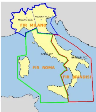
In Italy there are three large FIR (see Figure 1.1), Milano, Roma and Brindisi, which are provided by the Flight Information Services (or FIS) and ALS Alerting Service (or ALS). In order to control the FIR, four Area Control Center (or ACC) located in Milan, Padua, Rome and Brindisi. The airspace of ACCs is in turn divided into sectors, whose shape and size are consistent with the flow of traffic to manage, since a single Air Traffic Controller cannot physically handle all aircraft present in a FIR.
The airport in the international context
Figure 1.1: Italian FIR
1.2
The airport in the international context
Eurocontrol is an European organization which ensures flight safety, the ca-pacity, efficiency, Environment and security.
This civil and military organization, with has 28 member states, has as primary objective the development of an uniform and integrated pan-European system of air traffic management, according to the basic concept of the Single European Sky (SES), developing, coordinating and planning, with its member states, the implementation of strategies for pan-European air traffic management in the short, medium and long term.
At the international level, the rules for the operation and management of air-ports for civil use are, however, provided by ICAO[1] (International Civil Aviation Organization), in Montreal, Canada. ICAO is an independent agency of the United Nations, which was responsible to develop the principles and techniques of inter-national air navigation, on routes and airports, and to promote the design and development of international air transport to make it more safe.
International Air Transport Association[2] (or IATA), also in Montreal, is rather an organization of airlines that has developed, such as the ICAO, codes for the identification of the airports in the world. The IATA codes consists of three-letter,and they are published every three years on the IATA Airline Coding Directory. The codes are used by airlines for schedules, reservations, and baggage handling.
1.3
The phases of departure and landing in the life
cycle of a flight
Flight procedures, which an aircraft must follow in order to ensure safety are defined by international control entities (eg ICAO). These phases (Figure 1.2 ) are illustrated in brief below, although some events are optional (eg de-icing).
Figure 1.2: Flight Phases
The crew is on board and receives a series of information from ATC systems about the flight to be undertaken, such as the Flight Plan, the weather and so on. This phase is also called the Control of Airport: the aircraft is in contact with the Control Tower (TWR) authorizing it (at the time OFB1) to start the aircraft and move it from the parking zone to the assigned runway.
At the time Actual Time of Departure2 (or ATD) the aircraft starts the stage of take-off and climb, passing to the stage of En-route, in which it maintains
1
Off Block Time. The time at which the aircraft will commence movement associated with departure.
2The time that an aircraft takes off from the runway. (Equivalent ATOT – Actual Take Off
The phases of departure and landing in the life cycle of a flight
altitude and speed indicated on its flight plan. After passing through various areas of control, phase of descent begins. Each FIR may contain several TMA (Terminal Manoeuvring Area), in which the aircraft is accompanied during the final approach from Control Tower. After landing, the aircraft crosses the assigned taxiway pointing to the gate of competence or to the parking area (Apron). Upon completion of these operations and in correspondence with Actual of Block Time (or OBT), the airplane is taxiing to the holding point of runway indicated on the flight plan, and then it starts taking off, taking the SID (Standard Departure Route) corresponding its route.
These flight procedures show a well-defined life cycle of the aircraft that is briefly described in the following sections.
1.3.1 Pre-flight, Taxi and Take-off
This is the stage before the take-off, during which the aircraft is stopped at the gate indicated on the Flight Plan to allow the boarding of passengers (Figure 1.3).
Figure 1.3: Flight Phases
The crew is on board and receives a series of information from ATC systems about the flight to be undertaken, such as the Flight Plan, the weather and so on. This phase is also called the Control of Airport: the aircraft is in contact with the Control Tower (TWR) authorizing it (at the time OFB - Off Block Time) to start the aircraft and move it from the parking zone to the assigned runway.
1.3.2 Climb
After the phase of movement on the ground, at the time OBT (Off-Block Time), the pilot is authorized, by the control tower, to take off which will take place at the time ATD (Actual Time of Departure) only when the safety distance (Wake Vortex Separation) from all other aircraft will be granted.
Figure 1.4: Climb
Once taken off the plane, that is always in contact with the Control Tower (TWR), it passes through the phase of Approach Control that ensures a safe route towards the assigned aerovia (air route between the airport of origin and destination).
1.3.3 En-Route
Once taken off (Figure 1.5) the aircraft goes on along the assigned airway and is taken over by the Area Control Centre (ACC) which manages the Route Control.
An altitude and the path to follow is assigned to the aircraft, so that it always respect the safety distance (called separation), both horizontally and vertically, from other aircraft.
Close the airport destination, the aircraft is in Approach Control Phase during which it is driven into the descent alignment with the runway.
The phases of departure and landing in the life cycle of a flight
Figure 1.5: En-Route
1.3.4 Descent and approach
When the aircraft is on the path of landing (Figure 1.6) and the airport is close, it is managed by the Control Tower of the destination’s airport, which guide the aircraft during landing until the parking or the Gate.
Figure 1.6: Descent and approach
1.3.5 Taxi and Arrival
The landing is completed at the time Actual Time of Arrival3(or ATA). During this phase the pilot may use, if available, instruments such as PAPI (Precision
Approach Path Indicator) and ILS (Instrumental Landing System), which guide the approach to the runway.
Chapter 2
Problem Statement and State
of the Art
The airport system, for its role in public transport, must ensure that all op-erations (take-offs, landings, aircraft movements etc...) are completed safely. Ap-propriate authorities such as ENAC and ENAV, are delegates to ensure that these operations (both performed on the ground and in the air) are properly made. Such authorities have issued a series of regulations that govern the entire airport traf-fic (including departure and landing operations), from aircraft to means for the cargo. There are many modeling efforts and / or prototypes for scheduling such operations in order to maximize throughput, minimizing aircraft’s delay and work-load’s controllers, etc. . The purpose of this chapter is to present the problem of departures planning and show how it has been treated in the literature by several authors.
2.1
Departure Flight Scheduling
The Air Traffic Control (ATC) is a set of rules and institutions that contribute to make safe and ordered the flow of aircraft both on the ground and in the sky. In Italy, the role of the Regulator, (the authority that issues the regulations) is covered by the Civil Aviation Authority, while the ANSP (Air Navigation Service Provider, a company that provides air traffic services) is ENAV SpA. The ENAV emanates data aeronautical information essential for the operation of air traffic in
the form of publications AIP Italia [3] (Aeronautical Information Publication). These publications contain permanent aeronautical information concerning the national airspace, airports, organization of air traffic services and infrastructures. Examining AIP Italia publications one can identify a whole range of regulations that affect and limit the throughput (number of operations take off / landing in the unit of time, usually an hour), in order to ensure the necessary security to the aircraft flow.
The controllers in the control tower, which are responsible for the land traffic management, receive information on arriving aircraft a few minutes before they take off from the departing airport, so that they can prepare in advance a taxi plan from the landing runway to the gate. Compared to arrivals, planning for departing aircraft is processed directly in the Control Tower, and is ready in ad-vance with respect to the departure time, so that accidents can be easily handled. For each departing flight, defined as “scheduled”, a time slot assigned, consisting of a coordinated range of fifteen minutes, within which the aircraft must take-off. This slot, defined Calculated Take Off Time (or CTOT), is assigned by the Con-trol Flow Management Unit (or CFMU), an operational unit within EuroconCon-trol, designated to air traffic control with headquarters in Brussels (Belgium), in order to maintain a flow of constant traffic in all European air regions, so as to avoid the occurrence of congestion. Until a few years ago, the process of planning the arriving and departing flights was exclusively managed by air traffic controllers, that in situations of heavy traffic, were assisted by other controllers.
For several years, tools to help and support the work of auditors in planning operations runway are under study and development. Their aim is to provide a possible “planning” in accordance to plane delays, queues at the holding point, destination, state of the taxiway and time needed to cover them, and other vari-ables.
This schedule is processed trying to optimize the use of airport resources, re-ducing delays and minimizing waste.
In most airports, the runway is the bottleneck for an optimal planning of op-erations, since it is typically a shared resource between landing opop-erations, takeoff and crossing. A possible solution to this problem is to build new runways, but this choice cannot be adopted for both the high cost that the airport should support,
Aeroportual Safety Rules and Goals
and due to the lack of suitable areas. In addition, the boundaries of the airports usually have highly developed urban centers, whose populations raise legitimate concerns to preserve the environment from noise and pollution due to aircraft engines, by limiting the number of arrivals and departures (hence throughput), particularly at night, resulting in the loss of revenue from airports.
The term DMAN (Departure Manager ) means any tool that can optimize tail of take-offs, sharing the runway with landing and crossing operations. Stakeholders and various industrial partners gave the following definition of DMAN:
“DMAN is a planning tool that on the basis of the constraints and preferences, aims to improve the flow of departing from an airport, calculating the Target Take Off Time (TTOT) and the Target Start-up Approval Time (TSAT) for each flight”. The use of this tool in the airport context should give the following benefits: • improved on-time departures;
• better use of runway capacity;
• better information service to passengers (about delays and quantification of the delay);
• reduction of the workload of the air traffic controller;
• reduction of emissions, due to the queues decreasing at the holding point; • economic benefits.
The aim of this thesis is to define a mathematical model for the management of departures and implement a prototype of DMAN system.
2.2
Aeroportual Safety Rules and Goals
The management of airport traffic is, in general, subject to financial and op-erative interests of the various involved stakeholders, such as users of the airport (passengers, airlines, etc..) and providers of ATM services (airport authorities, air traffic controllers, etc..). In addition, there are legitimate concerns in order to preserve the surrounding environment from airport noise and pollution from engines on the aircraft. The objectives and interests can be mutually supportive,
and rivals in some cases. A certain level of security should be guaranteed, and the workload of the Air Traffic Controllers must be sustainable.
In summary, the main objectives of an airport system are:
• throughput (or capacity): optimize the use of shared resource (runways, taxiways, gates, etc.), minimizing the taxy and pushback time, and the de-lays in authorization (clearance) and pushback, implies an increase of the throughput;
• aircraft delay: minimizing any delays that may occur during the various stages prior to departure (boarding, refueling, cargo operation, etc.); • fairness: treat airlines with equity;
• workload: minimize the effort of controllers in managing the runway’s op-eration;
• environmental pollution: keep aircraft engines switched on as little as possible.
These objectives are subject to constraints in order to ensure that the runway’s operations are completed in safety. These constraints are divided in two categories:
• “universally recognized ”: common in all airport systems;
• “local ”: local to the particular airport (eg state of the runs at night); “Universally recognized” constraints, as resulting from regulations issued by local traffic control plan, are the following:
• Minimum separation between aircraft on the runway (Wake Vortex Separa-tion);
• Departure routes (horizontal and vertical separation in air); • Speed group;
Minimum separation between aircraft
2.3
Minimum separation between aircraft
Aircraft taking off and landing on the back generate a wake vortex (Figure 2.1), originated from the wingtips, which although of limited duration, can interfere the operations of any aircraft that follows.
Figure 2.1: Vortex behind the aircraft
The International Civil Aviation Organization (or ICAO), based on the MTOM (Maximum Take-Off Mass), has divided aircraft into three categories[4] (Wake Vortex Category):
• Light (L): MTOM of 7,000 kg or less;
• Medium (M): MTOM exceeding 7,000 kg but less than 136,000 kg; • Heavy (H): 136,000 kg or more.
An aircraft of category Light (or L) can take-off only two minutes after the take-off of an aircraft of category Heavy (or H). Similarly are defined time sepa-rations between an operation of landing followed by a take-off and vice versa. In Italy, ENAV SpA give a different definition of Wake Vortex Category [5], grouping the aircraft into the following four categories, three of which according to MTOM, and the category Super (or J) depending on the type of aircraft:
• HEAVY (H): MTOM exceeding 136,000 kg;
• MEDIUM (M): MTOM exceeding 7,000 kg but less than 136,000 kg; • LIGHT (L): MTOM of 7,000kg or less.
The separation times for these weight categories are described in the AIP Italy of Enav SpA.
2.4
Departures routes
The Departures Routes are also known as Standard Instrument Departure (or SID). These are procedures the aircraft must follow immediately after take off, as long as it remains in the vicinity of the airport. In particular, these procedures have been designed to allow the aircraft to leave the airport without obstacles (artificial or natural) that can be found closely, and to reach a Terminal Control Area (or TMA).
If a same SID is assigned to more aircraft a separation among the aircraft must be imposed, so as to ensure that the security distance is maintained even in the phase of En-route (Figure 1.5). In particular, the minimum horizontal separation of vehicles, checked with radar equipment, is five miles, otherwise the procedural separation is applied, whose minimum extension is normally not less than twenty miles (approximately thirty-seven km).
2.5
Calculated Take-off Time
In order to ensure the efficient use of airspace, Eurocontrol has set up a task force whose role is to manage air traffic in Europe, so to avoid congestion. This operation of supervision is fulfilled assigning each aircraft, which have to take-off, one time slot Calculated Time Of Take-off (or CTOT), within which it is authorized to take-off. It is important that the aircraft take offs within this time window, and in case the estimated time of departure is not within this range a new CTOT should be asked. In Europe, this window is defined by the five minutes before CT OT and ten minutes after.
State of the Art
2.6
State of the Art
The scheduling of departures planning for over a decade has become an impor-tant research topic in the context of Air Traffic Management (or ATM). Several researchers have focused their interest to these problems, as well as the most influ-ential European authority in this field, Eurocontrol, that has invested significant resource in order to promote several studies on scheduling departures.
The German Aerospace Research Centre [6] (or DLR) has developed a tactical concept of departures management and functional prototypes of DMAN (Depar-ture MANagement) system. NLR [7], the famous Dutch research institute special-ized in avionics and aerospace, introduce an approach based on the technique of Constraint Satisfaction Programming (or CSP) to solve this problem.
In 2003, Eurocontrol commissioned DLR to develop a prototype of DMAN, configurable for a given set of airports and used as a demonstrator stand-alone or as an operational tool in a real simulated ATC scenario. But it should be noted that despite the different formulations and solutions, fundamental issues regarding the efficiency of a certain approach, the concept of use and the benefits that can be derived, are not fully understood. In addition, due to the different types of airports, a more general approach and a formulation of the problem to be quite general.
There are several scientific papers in the literature, but in this context of anal-ysis, will focus our attention on some of these to show how the problem departure management has been addressed with different formulations. Anagnostatikis ([8], [9] and [10]), in departures planning considers also the eventuality of having to reschedule the sequences in relation to landing operations and crossing runway. In particular [8] and [10], the author presents a modeling based on the principles of linear programming, in which a multi-objective function is used in order to obtain a schedule of runway operations (methodology of single stage) . In [2] the same author deals the same problem dividing it into two subproblems, associated re-spectively with only two objectives, namely the throughput and the delay of the aircraft (dual-phase methodology). Atkin, Jason et al. in [11] and [12] present a mathematical model for the planning of departures based on the queues that are formed at the holding point. This approach has fallen on the specific Heathrow Airport, making it difficult to apply to other contexts airport. Instead, in [?], [13],
[14], [15] and [16] the problem of planning the departure is formulated with the innovative technique of Constraint Satisfaction Programming.
2.7
Single Stage Methodology
The problem of departures and arrivals planning is first formulated as an op-timization problem based only on the starting sequence. Therefore define:
• D the set of nD departures for which the optimal sequence s∗ will be found; • A the set of nAlanding aircraft;
• C the set of all known strong constraints (Wake Vortex Separation, SID, Priority, etc.) .
The optimization problem is expressed us:
s∗= arg min
s∈S(D,A,C)Q(s) (2.1)
where the function Q(s) measures the quality of sequence s and S(D, A, C) is the set of all feasible sequences of arrivals mixed at departures.
The max cardinality of sequences in S(D, A, C) is:
ns≤
(nA+ nD)! nA!
(2.2) where ns is the cardinality of the set S.
The relation (2.2) provides information about the space search that must be examined in order to find an admissible solution (or sequence). But as you can see, if you only need to plan take-off, maintaining constant the order of arrivals, the space search is still too large, and the search times are still computationally high. In addition, a method for the construction of the measurement function Q(s), which should evaluate the adequacy of each possible sequence respecting the objectives and constraints of the planning, it is not yet known. Then according to these considerations it is evident that an approach in the resolution of such problem, based exclusively on sequences of aircraft without considering the variable “time”, presents the disadvantage of being expensive in terms of resources and,
Single Stage Methodology
moreover, remains unclear the methodology of calculation of landing times and take-off of such sequences.
In front of such difficulties and, noting that both objectives and constraints are based on the time variable, a most appropriate approach for these planning problems is to consider the time. For example, it is sufficient to map each taking-off operation exactly at a time, which could be the take-taking-off time or the initial occupation time (we can imagine a sequence as an array of take-off time, each of which represents an occupation time), assuming that the width of these intervals is known.
So, defined a vector t consisting of all take-off time of aircraft contained in the set D, the time optimums vector is given by:
t∗= arg min
t∈T (C)Q(t) (2.3)
where Q(t) is an evaluation function that reflects the goals of planning and T (C) is the n-dimensional space of solutions subject to strong constraints. But even this approach involves complications. In fact is noted that the set of con-straints C contains both the demands of minimum separation between take-offs and information concerning arrivals, and therefore this implies that the space T (C) is a non-convex set and a disjoint set. To better understand what is stated we consider for example the case in which the constraints are:
• minimum separation between two take-off operations t1 and t2 of 120 sec., denoted by c1 : |t1− t2| ≤ 120;
• the occupation interval of the runway for an arrival is between 120 and 165 sec., denoted by c2: tA1 = h120, 165i ;
• departure marked “1” is supposed that, for some reason, can not reach the runway earlier than 100 sec..
The disjoint, non-convex and two-dimensional space T (C) is shown in Figure 2.2.
Figure 2.2: An example of a two-dimensional, non-convex, disjoint search space T(C) (white area)
It should be noted that, in addition to the difficulties related to the properties of T (C), it could happen that the function Q(T ) is multi-modal, with several local minima.
It follows that the optimization problem is too complex and computation time too high. From what it has been seen, both the approach based on the sequences and on the time are not adequate for a planning problem, in fact the former is insufficient, the second is too complex.
A “mixed” formulation may provide, under certain conditions, a basis for re-solving this problem. Then, for each sequence S an optimization based on the time could be considered; in this case the solution space is not defined only by the string constraints, but also by a series of inequalities each of which governs a pair of take off times:
U (s) = {ti≤ tj ← ipsj ∀i, j ∈ s} (2.4)
which indicates that the take-off time of aircraft i is lower than of the aircraft j if i precedes j in the considered sequence.
Therefore given the evaluation function Q(t), the vector of optimum take-off times t∗ for a specific sequence s is expressed by:
t∗= t∗(s) = arg min
Single Stage Methodology
and the optimal sequence s∗ is achieved minimizing the value of Q(t) among all feasible sequences in the set S(D, C):
s∗ = arg min s∈S(D,C)Q(t
∗(s)) (2.6)
The global optimal vector of take off time is then given by: t∗∗= t∗(s∗) = arg min
s∈S(D,C)t∈T (C,U (s))min Q(t)
2.7.1 Multi-objective modeling
The goal of the system are transformed into objective functions indicated with qi(t). The latter must comply with the following properties:
qi(t) ≥ 0 qi(t) = n X j=1
qij(tj) (2.7)
Furthermore each of these q(t) is defined such that lower is its value and more the solution satisfies a certain goal or less is violated a certain weak constraint. Although you can define different objective functions for each of the goals of the system we will evaluate only the most influential: the throughput, defined as the ratio between the number of departures nor the time required to perform these operations and is related to the time of take-off of the last aircraft in optimal sequence S, impartiality (fairness) and the taxi times. As regards the capacity, it is natural, from the given definition, write it as q(t) = max(t). A more appropriate definition of this objective function could be the following:
q(t) = n X
j=1
bjτjp , p > 1 (2.8)
where τj = tj− t0is the time relative to the aircraft j, with t0 the current time, bj is a vector of weights and p is an appropriate parameter. As you can see, in the most general case, the objective function is not linear because of the presence of p.
A mathematical formulation of the objective function that expresses taxiing time based delays encountered at the end of the process of taxiing, is as follows:
q(t) = n X
j=1
where δT,i(tj) = tj−tRT O,j is the delay due to the delay of aircraft j and tRT O,j is initial time of take-off for the same aircraft.
With regard to fairness, that ensure equal treatment of passengers and airlines, can be formulated in terms of delay for the aircraft j, between time ready for pushback tRP B,j, and the time planned to pushback tP P B,j . In particular, since this delay does not affect the timing of taxiway, the objective function is given by a relative progressive evaluation of such delays, written as follows:
q(t) = n X
j=1
δP,B,j(tj)p , p > 0 (2.10)
where δP,B,j(tj) means the delay of the aircraft pushback j.
A remark should be made on the weak constraints, defined as a function of time and which translate the constraints of flow to earth, whose violation in order to generate a solution is allowed (eg. CFMU). Such constraints, can be defined with appropriate functions that measure the degree of their violation. Therefore, an evaluation function of violations of constraints can be written as:
q(t) = n X
j=1
c(τj)δj(tj, tc,j)p p > 0 (2.11)
where tc,j is the estimated time of departure (is +∞ when a departure j is not subject to any constraint), and
δj(tj, tc,j) = 0 tj ≤ tc,j tj − tc,j tj > tc,j (2.12)
is the amplitude of the constraint violation.
2.7.2 Planning: solution
The objective functions may be useful for both evaluation of the goals and constraint violation. It can happen that some of these can contradict each other and therefore sometimes minimize one could result in the growth of the value of the other. In order to have different objective functions, the scheduling problem formulated as a vector optimization problem with the right compromise between these.
Double Stage Methodology
A general model for the planning function Q(t) is represented by a linear com-bination of the individual objective functions qi(t):
Q(t) = aTq(t) (2.13)
where
q(t) = [q1(t), ..., qr(t)]T (2.14) is a vector of r objectives functions and
aT = [a1, ..., ar] (2.15)
is the corresponding weight vector with: ai≥ 0 ∀i ∈ Nr = {1, 2, ..., r},
r X
i=1
ai = 1 (2.16)
Therefore, the optimal solution becomes a function of the weight vector a: t∗(a) = arg min
t∈T (C)Q(a, t) (2.17)
s∗(a) = arg min
s∈S(D,C)Q(a, t
∗(s)) (2.18)
The given formulation of the problem of takeoff management refers to a “static” airport model, in which all the essential information are always available when required. However, such a problem is fallen in a real airport environment that is dynamic by nature, and where the information is not always available when required.
Therefore, the uncertainty created in these situations is reflected in formulated model negating the performance and operation.
To find the optimal solution s∗, the use of a search tree, and the technique of Branch & Bound appear to be the most appropriate, since only a subset of the possible sequences is examined.
2.8
Double Stage Methodology
The dual stage methodology divide the above problem into two sub-problems, said phases (or stages):
S L H
S 60 60 60
L 60 60 60
H 120 120 90
Table 2.1: Example of Wake Vortex Separation matrix
• first stage: the goal is to maximize runway capacity (throughput), without violating the wake vortex separation and delay due to operations of runways crossing;
• second stage: the goal is to minimize the delay without violating the con-straint imposed by CTOT (Europe) or EDCT1(America).
2.8.1 First stage
The purpose of the first stage is to optimize the throughput generating se-quences of take off, and considering as main time constraints wake vortex separa-tions. Also are considered “mixed” runway operations, in the sense that in addition to departing aircraft, we take into account also arriving aircraft and “crossing” op-erations.
2.8.2 Constraints
The generated take off sequences in the first stage must comply the Wake Vortex Separation constraints, ie a minimum separation time between an operation and the next must be guaranteed. The set of the time intervals can be represented as a matrix (Table 3.1), whose rows correspond to the possible categories of weight of an aircraft that precedes another while columns express weight category. The value resulting from the intersection between row and column corresponds to the minimum separation time that must be guaranteed between the two operations.
Two additional constraints that influence further throughput sequencing are: • the maximum number of landed aircraft that are waiting for a clearance to
cross an active runway (where they are needed);
Double Stage Methodology
• the maximum delay that an aircraft landed and waiting to cross an active runway can absorb.
The limit values of both constraints are input data to the planning system, and can be modified in real time by the planner.
2.8.3 Objective Function
Maximize capacity means minimizing the time in which the last operation are authorized take-off. Therefore, the formulation of the objective function is the following: let NAand ND respectively the total number of arrivals and departures, and N = NA+ ND the total number of mixed operations on the runway(s) during the current scheduling window (scheduling is performed dividing the time into smaller intervals of equal amplitude and considering operations that fall within that range).
Minimization of the time of the last takeoff is given by:
min max tDi 1 ≤ i ≤ ND (2.19)
2.8.4 Sequences’s Classes
It is assumed that the schedule of arrivals is known a priori. Once the aircraft landing and decelerate, is sought authorization for the operation of “crossing” (if necessary) in the event that needs to cross an active runway, and the instant of time at which start the operation. These time instants are estimated on the basis of the weight of the arrival aircraft and taxiing constraints. Therefore maximizing requires careful planning departures and runway crossings (if they are required).
2.8.5 First Stage Output
The output of the first phase is a matrix containing all possible sequences of aircraft, ranked, with the property of maximizing the throughput of the runway.
The above matrix is namely “matrix CS” (matrix of Classes of Sequences). CS = class sequence 1 class sequence 2 ... class sequence m (2.20)
The first class sequence in the matrix ensures the highest throughput and, for this reason, it is identified as Target Class Sequence (or TCS).
2.8.6 Second Stage
The second stage optimizes the delay of each aircraft. In the previous stage a matrix of class sequences has been generated and it ensures, in addition the best throughput, that the right separation time (according to the Wake Vortex Separation) are fulfilled. The first class Sequence of the matrix becomes the Target Class Sequence (or TCS), and it is used as a basis to generate the schedule. In fact, in this stage, the aircraft are assigned to each slot, trying to minimize the delay of take-off. If the selected TCS is not feasible solution (since the constraint of the second stage are not satisfied, the new TCS becomes the next row in the matrix. The decision variable Xij used for the formulation of this second stage are defined by:
(
Xij = 1, if aircraft i occupies slot j Xij = 0, otherwise
The basic requirement is that no aircraft is assigned to a slot that can not physically occupy, ie time slots earlier the time in which the aircraft can reach the runway. For example, if the air plane takes a time equal to 900 (seconds) to reach the runway and the time in the middle point of the fist two slots in the TCS is less than 900 (seconds), then the aircraft can not occupy the slots 1 and 2 in the final solution. In this case, this type of constraint is expressed by:
Xij = 0, for slot j = 1, 2
A further constraint is given by the same sequence of slots classes, ie if an aircraft belongs to the Large (or L) wake vortex class, then it can only occupy the
Double Stage Methodology
slots of type L within the TCS. This constraint is translated as: X
j
Xij = 1, ∀ slot j ∈ L
where L is the set of slots of type Large within the TCS. In addition, each aircraft must occupy only a single slot:
NS
X
j=1
Xij = 1, ∀ aircraft i
where NS is the total number of slots in the class sequence. Moreover each aircraft may be assigned at most one slot:
ND
X
i=1
Xij = 1, ∀ slot j where ND is the numbers of aircraft planned for take-off.
The operational constraints, such as the estimated time for the authorization of a departure EDCT (Expected Departure Clarence Time) or DSP (Departure Sequencing Program), restrict the time available for the plane take-off:
tEDCTi1≤ tDi ≤ tEDCTi2 or tDSPi1 ≤ tDi ≤ tDSPi2
where tEDCTi1, tEDCTi2, tDSPi1 and tDSPi2 are the times (as defined by ATC) that determine the time window of the EDCT (15 minutes) and the DSP (3 minutes) for the i-th plane.
A heuristic method may be used to transform the time window in a take-off slots. Let us consider the take-off position of each plane as function of the variable decisionPNs
j=1j ∗Xij then the previous constraints are formulated as an acceptable range of slots:
sEDCTi1≤PNj=1s j ∗ Xij ≤ sEDCTi2 or sDSPi1 ≤PNj=1s j ∗ Xij ≤ tDSPi2 where X, Y, Z and J are the final values of the take-off slot (defined by ATC) for the i-th flight, which define the windows of the slot of take-off EDCT or DSP. Other types of constraints (such as in airplanes for rescuing) are modeled in the form of upper limit on the position of the take-off sequence, ie:
Ns
X
j=1
or in terms of inequality constraints between different flights: Ns X j=1 j ∗ Xij ≤ Ns X j=1 j ∗ Xkj
The operational constraints ”Miles In Trail” (MIT) and ”Minutes In Trail” (Mint) require separations between aircraft en route, and are defined in terms of separation of time at the point of take-off:
|tDi− tDj| ≥ ∆Tij
where ∆Tij is the minimum separation time of the take-off point between the airplane i and j that have a restriction “In Trail”.
The constraints MIT (or MinT) can be defined as a function of the minimum separation required in the sequence of take-off ∆Xik between the flights i and k and the spatial position of the slots of the class sequence:
Ns X j=1 j ∗ Xij · Ns X j=1 j ∗ Xkj ≥ ∆Xjk ⇒ ( PN s j=1j ∗ (Xij· Xkj) ≥ ∆Xik PNs j=1j ∗ (Xij+ Xkj) ≥ ∆Xik
An huge task for air traffic controllers is to ensure the “fairness” between airport users; for this purpose a constraint called “impartiality”is introduced. It is defined as the maximum displacement of the off position (MPS – Maximum take-off Position Shifting) misleading the adoption of a policy of “First Come First Serve”. The value of MPS can be predetermined by ATC or by airlines and gives the acceptable positions in the take off sequence for each departure. For each aircraft i, indicated with XP Bi and XT Oi, respectively the position in the sequence of pushback and the position in the sequence of take-off, one has the following relationship: |XP Bi· XT Oi| ≤ M P S ⇒ ( −PNs j=1j ∗ Xij ≤ M P S − XP Bi −PNs j=1j ∗ Xij ≤ M P S + XP Bi where the values MPS and XP Bi are known a priori.
2.8.7 Objective Function
The objective of this second phase is to minimize the delay for each aircraft, comparing the first time available in the class sequence with the estimated time of departure issued by the airline to which it belongs.
Double Stage Methodology
In the general case of use of a runway, T Oni the original times of arrival (when the aircraft touches the ground), T Xi runway crossing times of these arrivals, and T Of fj times ’objective’ departure (take off authorizations), as the values of the midpoint of the slot class, are defined.
Similarly for each aircraft delays (intended as time differences) between the actual landing, the crossing, time of take-off and the corresponding values closest possible (the temporal midpoint of each corresponding slot), respectively defined as EOni , EXi and EXOf fi. The delay value for each operation indicates how it deviates from the nearest time to perform this operation. The total delay is formulated as: ( ND X i=1 |T Of fi(xi)−EOf fi|kD+ NA X i=1 |T Onj−EOnj|kA+ NA X i=1 |T Xm−EXm|kX) (2.21)
where 1 ≤ i ≤ ND and 1 ≤ j, m ≤ NA with ND the total number of departures and NAthe total number of arrivals; xi is the position of the aircraft i in the slot and kA, kD and kX are parameters used to penalize delays of specific flight with kA, kD, kX ≥ 1.
Therefore we aim to minimize the objective function in (2.21). In particular, if we aim to minimize only the delays associated with departures we obtain:
min ND
X
i=1
|T Of fi(xi) − EOf fi|kD dove 1 ≤ i ≤ ND (2.22)
The output of the second stage is a matrix AS (Aircraft Schedule) in which each row represents a scheduling of the aircraft. The matrix is sorted for delay. So the first line indicates the best schedule:
AS = [aircraf t schedule 1, aircraf t schedule 2, ..., aircraf t schedule N ]
2.8.8 Approach based on CSP
A number of problems in Artificial Intelligence are classified as Constraint Satisfaction Problem (or CSP) problems. The classical combinatorial, resource allocation, planning and time reasoning problems, which are exactly solved by techniques of CSP.
Formally a problem of CSP is defined by a set of variables, indicated by X1, ..., Xn, and a set of constraints C1, ...., Cn.
Each variable Xi belongs to a non-empty domain of possible values. Instead a constraint Ci = C(Xi1, ..., Xik), between k variables, is a subset of the cartesian product Di1× Di2× .... × Dik that specifies the values of compatible variables.
A statement of the problem is given by an assignment of values to some or all of the variables, say X, which is called ’consistent’ if any of the constraints are not violated.
When the assignment involves all the variables is called “full”: therefore, con-sequently, we defines “solution of the CSP” a complete assignment that satisfies all constraints.
When a goal is added to a CSP, the problem obtained is defined Objective Constraint Programming (or COP), in which the aim is to find an optimal solution according to a preassigned evaluation criterion.
Therefore a resolution algorithm for any CSP problem can be used in an equiv-alent manner to solve a COP simply adding a further variable that represents the objective function. Each time a solution is found, the solver imposes the constraint that any further solution found has the value of the better objective function, and if this procedure leads to a failure then the current solution is the optimal one. The technique of resolution of the CSP makes use of a decision tree that is obtained by matching at every level the assignment of a variable, according to a predetermined order, and at each node the choice of the value to be assigned to the variable cor-responding to the level where the node is located. It is therefore evident that each leaf of the tree represents a different combination of values assigned to the vari-ables. The leaves associated with assignments compatible with all the constraints of the problem are solutions of the problem. The search for a solution is therefore equivalent to the exploration of the decision tree associated with the problem, in order to find a leaf with an assignment compatible with the imposed constraints. CSP formulation of the problem of scheduling of take-offs
For the formulation of the scheduling problem in terms of CSP first identify the variables, their domains and constraints in the domain context. The basic object considered in the model is the flight. An aircraft, its crew and its flight plan that contains general information such as departure airport, destination, etc. are associated to each flight.
Double Stage Methodology
The set of flights for planning is {F1, F2, ...FN}. For every flight Fjthe following date are known:
• gate and parking bay;
• destination point, ie the exit point (TMA – Terminal Manoeuvring area); • CTOT (Calculated Take-Off Time). There exist two typologies of flight, ie
scheduled and not. The first need to take-off within the time given by the CFMU, the latter are not the subject of study;
• flight plan;
• the technical characteristics of the aircraft. The output for every flight Fj we want to calculate:
• the take-off time (TTOT – Target Take-Off Time), which is the point in time at which the aircraft should start the race on the runway;
• a sequence number, which indicates, for a specific track, the order of depar-ture of the aircraft;
• a route SID that allows the aircraft to reach the exit point.
The set of constraints specifies restrictions for a single flight or between two of them. In fact, precisely, the constraints are modeled through the relationship between the characteristics of a single flight and its time position or by relationships between two or more flights. Hard Constraint (cannot be violated) as the Wake Vortex Separation, the Departure Routes (SID) and the Speed Group are obliged to be satisfied in order to avoid dangerous situations, but instead the weak constraints (can be relaxes), such as the pilot’s flight plan and priorities due to the long delay in aircraft may be violated, even if it is not, usually, the preferred solution.
As an example of a formulation of constraint through the technique CSP con-sider the case in which an aircraft class Light should be scheduled at least three minutes after the previous (because of the wake vortex). We can say that the air-craft associated with the flight Fi is heavier than the one associated with Fj and the only situation in which the Fj could start before Fiis keeping them on separate
runways. The corresponding constraint, here indicated with Ck, is written as a set of four conditions to be avoided:
Ck= ∀Fi, ∀Fj con Fi6= Fj N OT (R(Fi) = R(Fj)) OR (ttakeof f(Fi) > ttakeof f(Fj)) OR (w(Fi) ≤ w(Fj)) OR (ttakeof f(Fi) + 3 ≤ ttakeof f(Fj))
where Fiand Fj are two flights to be scheduled and R, w, ttakeof fare functions that return respectively the runway allocated, the weight class of aircraft and the take-off time. Considering the routes SID as a set of “nodal” points, the corresponding constraint, understood as separation between two aircraft (in order to prevent overload situations on these routes of “fitting” as well as for safety reasons) can be written as following: Cs= ∀Pi, ∀Pj con Pi 6= Pj N OT (sameSID(Pi, Pj)) OR N OT (f ollows(Pi, Pj))
OR (tover(Pi) + f lying time(Pi, Pj) = tover(Pj))
Here Pi and Pj are the points related to the two aircraft, same SID and follows are two functions that control, respectively, if the two points belong to the same SID, and if the two points follow each other, tover is a function that returns the instant of time in which a flight crosses a “nodal” point.
The National Aerospace Laboratory (or NLR) has developed a tool to generate the sequences of the departures, known with the name of Mantea Departure Se-quencer (or MADS) [17]. MADS ensures that each aircraft take offs in its CFMU slot, respecting the separation and not overloading the sectors of airspace.
MADS was made by examining five categories of constraints: • separation constraints (Wake Vortex Separation);
• constraint on the use of the runway. For example in airport with more runways, for each of them are indicated: availability, size, surface conditions, equipment and weather conditions.
Double Stage Methodology
• constraints of Terminal Manoeuvring Area2 (or TMA) and En-Route. It is necessary to ensure the constraints of separations in air (such as the separa-tion SID).
• time constraints: we must ensure that each aircraft take offs on its time slot (CFMU slot).
The technique used to develop this tool is already consolidated and is known in Operations Research as Constraint satisfaction Programming (CSP). This tech-nique allows you to describe the problem using a set of variables, each of which is associated with a set of possible values. Constraints define the combinations of values of variables that are not allowed (for example two aircraft cannot take-off at the same time and on the same runway). A solution consists of a sequence of values associated with the variables, such that all constraints are satisfied. This solution, if it exists, is determined starting from an initial search space, with the technique of backtracking: the idea is to restrict as much as possible the domains of all the variables through the propagation of constraints. At the end of this operation the following situations can occur:
• a solution was found;
• one or more variables have no values: there are some constraints violated; • the search space may still contain solutions, therefore the algorithm continues
in the search for a solution (propagation of constraints).
This type of research involves a solution or a failure. Sometimes while using the CSP search space is too much reduced, it may happen that the number of valid sequences is still huge, and therefore it becomes necessary to create heuristics to speed up the search process. It is also important to initialize the algorithm, or choose the variables right place to start the search. In the literature there are several strategies, including that to independent domains, very fast, and that in domains dependent that in the case of the problem of departures requires a special heuristics to obtain a fast convergence to the optimal solution.
2Terminal manoeuvring area in Europe, is an aviation term to describe a designated area of
2.9
Approach based on queueing theory
The following approach, proposed in [11] and [12] has been designed for Heathrow Airport in London, composed by two runways, which is among the busiest in Eu-rope and is situated in a very small portion of land. It aims to increase the runway capacity according to a set of constraints and ensuring airport security.
2.9.1 Application context
A schematization of the two runways of Heathrow is shown in Figure 2.3:
Figure 2.3: The Layout of London Heathrow Airport
In this figure we highlight four “terminal” of which the first three, indicated by T 1, T 2, T 3, are located between the two runways, while the fourth, T 4 is south of the track labeled 27L. The objects labeled with HP are called “holding points”. Within these physical structures the runway controller can reorder the aircraft before they reach the runway.
The holding points can be identified as queues, ie points where aircraft are queued before entering the runway. If there are many different queues revenue, the ground controller attempts, starting from an initial entry order of the aircraft queues in the holding points, to direct the next aircraft to the HP “tail cheaper” (then running load balancing operation, so as to maximize the capacity of the track). Such operation is not only very difficult, but it can be repeated a limited number of times: this is said constraint of holding points.
Approach based on queueing theory
As for other proposed formulations, constraints considered for airport security, in this approach, are still the Wake Vortex Separation, the safety distance for routes SID, Speed Group for the initial calibration of the separations and CTOT.
2.9.2 Heuristics for the assignment of path
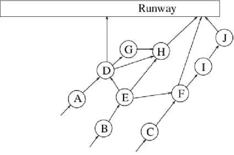
In reference to the runway 27R shown in Figure 2.3, a typical graph of the waiting point (HP) is shown in Figure 2.4. Each node represents a valid location
Figure 2.4: An example of holding point network structure
for the aircraft, while the edges represent their transitions through nodes within the holding points.
A valid transverse path consists of a sequence of nodes, interconnected by arcs; the first node of the sequence is the input in the waiting point, the end node is instead the runway. Therefore paths within the holding point are determined using an appropriate heuristic based on how fast an aircraft needs to arrive at the runway.
2.9.3 Departure Scheduling Algorithms
The Basic Search Algorithm
Rather than modeling the movement within the queue positions, the algorithm finds solutions that indicate only the order of take off. Once fixed the order of take off, the paths of the aircraft through the structure of the HP are assigned heuristically. A scheduling is considered “feasible” when all aircraft arriving on the track in the correct order. All of the search heuristics that has been investigated had the same basic format but differed in the details. The full algorithm for the basic search is as follows:
The search algorithm of solutions consists of the following steps:
1. start from the initial solution determined by the order in which the first aircraft arrives in the holding point. This solution is already “feasible” as it does not require the adjustment;
2. assigns heuristically paths for each aircraft within the holding points; 3. through an algorithm of “feasibility” ensure that the order of take-offs is
correct;
4. evaluate the cost of the solution;
5. accept or reject the candidate solution. In this step, you can apply different methods of meta-heuristic search (local search algorithms as the first de-scent, the steeper dede-scent, tabu search, simulated annealing) whose solution becomes the new current solution if it is accepted;
6. if the number of possible evaluations has been reached then the algorithm stops and the best solution hitherto found; otherwise it selects the one close to the current solution and the algorithm repeats starting from step 2.
Search Algorithms First Descent Algorithm: this is the most simplistic algorithm. Each new solution is accepted only if it is better than the current solution.
Approach based on queueing theory
Stepeer Descent Algorithm: The steeper descent algorithm selects fifty candidate solutions at a time. Each candidate is evaluated and the best of the feasible candidates is adopted. The best candidate is adopted even if it is worse than the current solution, which means this is more than a strict descent algorithm. This gives the algorithm a limited ability to move out of local optima but no method to avoid it moving straight back to the local optima it just left. Evaluations of candidates are expensive so the searches are limited to a number of evaluations rather than a number of iterations. This means that the first descent algorithm runs for fifty times as many iterations as the steeper descent algorithm.
Tabu Search Algorithm: The tabu search algorithm is similar to the steeper descent algorithm except that it maintains a list of tabu moves. When a move is made, the reverse move is added to the tabu list to ensure that the search does not go back to where it came from. The reverse move that is recorded will stop any move which would put all of the aircraft that moved back into the absolute positions they previously occupied.
Simulated Annealing algorithm: If the cost of the new solution is less than the current one, then the new will always be accepted, while if it is greater there is still a chance of being accepted. So if we denote by Dcurrthe cost of the current solution and Dcandthat of the candidate solution, then it will be accepted if Dcand < Dcurr .
2.9.4 Formal mathematical model
Let n be the number of considered aircraft, i ∈ {1, ..., n} an integer that rep-resents an individual aircraft, ai its position in the order of arrival at the waiting point (so that if i is the first to arrive then ai = 1 ) and ci its position in the take-off (so that if i is the second aircraft to take off then ci= 2 ).
We introduce the following integers, referring to the generic aircraft: • ti, the internal path to the waiting point;
• vi, weight class; • si, speed group; • ri, the SID;
• hi, the instant of time in which it enters the waiting point; • di, the scheduled time of departure;
• bi and li, interval bounds corresponding to the time CTOT;
• max(0, ci− ai) indicating the positional delay accumulated by each aircraft that i is overtaked;
• di − hi that expresses the delay to the waiting point, ie the time spent by the aircraft i within the waiting point.
We define two functions V (vi, vj) to calculate wake vortex separation, based on the weight classes vi and vj , and R(rj, sj, ri, si) to calculate the required separation based on the routes SID, ri and rj, and the group velocity, si and sj, for aircraft i and j. Both functions V and R give standard values of separation in accordance with the current regulations. Note that the ground controller has a certain flexibility, in the case there are clear weather conditions, to reduce the separations given by R(rj, sj, ri, si).
Unlike the functions for the routes SID and speed group, the function related to wake vortex separations satisfies the triangle inequality, ie V (vi, vj) + V (vj, vk) ≥ V (vi, vk) for aircraft taking off in the order i, j, k; therefore it is not possible to guarantee that all separations are maintained only by ensuring sufficient separation between adjacent take-offs. For example, consider a scenario in which a start “slow” aircraft is directed to north, followed by another “faster” directed to south, in turn followed by an other “faster” direct to north. As the two trajectories diverge between north and south, departure that consecutively follow these trajectories require a separation of one minute, due mostly to a difference in weight classes. A fast aircraft headed north following a slow also directed it towards the north however, requires a separation of three minutes.
ei is defined as the lowest take-off time for which all the separations are guar-anteed and is given by:
e′i = ( 0 maxj∈{1,...,n|}cj<c(dj+ max(V (vj, vi), R(rj, sj, ri, rj))) if ci= 1 if ci ≥ 2 (2.23)
Approach based on queueing theory
For each aircraft a transverse path ti is assigned heuristically , through the struc-ture of the holding points and defining a suitable function T (ti), returning the minimum time in which an aircraft i transversely crosses the holding points along the route ti .
Given the time hi, in which the aircraft arrives at the waiting point, the lowest time it can reach the runway and take off is given by hi+ T (ti) ; in particular the time of take-off can be predicted through the following relation:
di= max(ei, hi+ T (ti), bi) (2.24) For the constraint on the time CTOT defines an evaluation function C(di, bi, li, hi) that penalizing those schedules that put planes at the ends of the time interval defined by CTOT. The function C(di, bi, li, hi) has a complicated expression, it takes into account different functional cost which evaluate the delay and introduces factors that allow deviations of scheduling the time of predicted takeoff.
The objective function to be minimized takes into account the total accumu-lated delay to the holding point, the delay of positioning and eventual failure of the time constraint imposed by CTOT, and is given by:
n X
i=1
(W1(di− hi) + W2(max(0, ci− ai))2+ C(di, bi, li, hi)) (2.25) where W1 and W2 are appropriate weights.
Two Stage Algorithm: Formal
Model
3.1
Introduction
The proposed modeling approach was inspired by the works of I. Anagnostakis ([8] and [9]), in which some techniques of classical operations research are used. In particular, in [8] it is shown the ”Single Stage” methodologie in which the planning function Q(t) is a linear combination of individual objective functions q(t)i, each of one schematizes any goal of the system, while in [9] the original scheduling problem is splitted in two sub-problems or stages. In the first one the goal is to maximize the runway throughput (or capacity) while in the second one it tries the minimize the delay of each aircraft departure.
By analyzing in detail the differences of the two previous methodologies we decided to follow ”Two Stages” approach, since the computation times are lower than those obtained with previous approach, and the space of feasible solutions has lower cardinality. Moreover, this kind of methodologie allows us to treat the objectives and constraints separately, increasing maintainability and allowing to manage more efficiently and dynamically insertion of new constraints.
Here, initially a mathematical formulation for the case of single-runway airport was defined, then an algorithm for multi-runway management, considering the special case of independent runways, has been planned and integrated.
Two Stage Algorithm
3.2
Two Stage Algorithm
The goals commonly recognized by the airport system are:
• maximization of throughput, defined as the number of aircraft that can take off in the considered time window;
• minimization of the delay of individual aircraft: the planned time of take-off (Estimated Take-Off Time) shall not differ much from the target take-off time — TTOT (Target Take-Off Time) — calculated by DMAN;
• minimization of the workload of the controllers in the management of the runway operations;
• fairness, i.e. to treat all the airport users (airlines, passengers, etc.) in the same way;
• minimization of environmental pollution,keeping the engine running as little as possible;
However, since it is difficult to formulate some of these objectives we focused attention only on the following objectives:
• maximization of throughput;
• minimization of aircraft delays, considering the below constraints: – Wake Vortex Separation;
– Calculated Take-Off Time (or CTOT); – Estimated Take-Off Time (or ETOT)1;
– aircraft priority, i.e. the requirement that aircraft take off as soon as possible.
Both steps of the algorithm are formulated through a linear integer program-ming model. In a generic problem of Integer Linear Programprogram-ming (or ILP) the objective and constraints are expressed in terms of real linear functions, whose
1