DIPARTIMENTO DI INGEGNERIA DELL’INFORMAZIONE
Corso di Laurea Magistrale in Computer Engineering
Implementation of a suite of components for
Software Defined Radio using an SCA-compliant
framework
Tesi di Laurea
Candidato: Relatori:
Fabio Del Vigna Prof. Marco Luise
Prof. Mario Giovanni C. A. Cimino
Ing. Carmine Vitiello
The aim of this work is to introduce Software Defined Radio (SDR) technology, present an open source SCA-compliant framework whose name is Redhawk, which derives from the OSSIE project and describe an implementation example of some processing instances. Since in SDR applications it is necessary to run the same software on different hardware, portability becomes the main important aspect in the development of software radio applica-tions. The use of a SCA-compliant framework solves this issue making hardware transparent to the programmer and reducing time and costs of code development.
This aspect can be exploited for prototyping applications quickly without the need of a spe-cific hardware or testing new standards and protocols.
We will introduce some basic concepts of SDR, of the SCA architecture, based on CORBA, and Redhawk. We will then talk about of the implementation of a suite of components, writ-ten by using Redhawk IDE and C++ programming language. These will be tied together to form an application called waveform.
We will also present the results obtained by enforcing a certain level of parallelism in our algorithm to speed up computation in Redhawk components and boost performances against a more simpler non concurrent implementation of the same algorithms.
Abstract 4 1 Introduction 10 1.1 What is SDR . . . 10 2 Overview on SDR 12 2.1 History . . . 12 2.2 SDR paradigm . . . 13 2.3 SCA standard . . . 14 2.3.1 CORBA . . . 16 2.3.2 OSSIE . . . 18 2.3.3 GNU Radio . . . 20 3 Redhawk 22 3.1 Redhawk Core Framework . . . 22
3.2 IDE . . . 22
3.3 Sandbox . . . 23
3.4 Components . . . 25
3.5 Devices and Device Manager . . . 31
3.6 Domain Manager . . . 31
3.7 Installation . . . 32
3.7.1 UHD driver . . . 33
3.7.2 RTL . . . 34
4 Components 35 4.1 Convolutional encoder and Viterbi decoder . . . 35
4.2 Mapper and Demapper for QAM and PSK . . . 36
4.3 Spreader and Despreader . . . 40
4.4 Puncturer and Depuncturer . . . 42
4.5 FFT/iFFT . . . 42
4.6 Converters . . . 43
4.7 Rate Adapter . . . 43
4.8 Random Generator . . . 44
4.9 Write and Forward . . . 44
4.10 Scrambler . . . 44
4.10.1 Scrambler for symbols . . . 45
4.11 Block Interleaver . . . 45 4.12 Convolutional Interleaver . . . 46 4.13 Delay Estimator . . . 48 4.13.1 Timing Recovery . . . 49 4.14 Packetizer . . . 49 4.15 Noisy Channel . . . 50 4.16 Delay Generator . . . 50 4.17 ConstMultiplier . . . 51
4.18 Wide Band FM Demodulator . . . 51
4.19 De-emphasis filter . . . 52
4.20 Hamming filter . . . 52
5 Parallelism 53 5.1 What is parallelism . . . 53
5.2 How to reach parallelism . . . 54
5.3 Filter . . . 54
5.4 Performance comparison in filtering . . . 57
5.5 Oversampler and Decimator . . . 59
5.6 Delay Estimator with parallel architecture . . . 60
6 Waveforms 61 6.1 How to build a waveform . . . 62
6.2 A real example . . . 63
7 Conclusions 66 7.1 Future perspective . . . 67
A Filter code 69
B Resampler code 80
Acronyms 87
2.1 Classification of software radio devices . . . 14
2.2 Operating Environment and relation with the Application Environment Profile 15 2.3 SCA Architecture Layer . . . 16
2.4 CORBA client-object interaction . . . 17
2.5 Client performs a method invocation on a remote object through a remote reference . . . 18
2.6 The object receives a method invocation . . . 19
2.7 CORBA middleware in SCA . . . 20
3.1 Redhawk IDE and the Sandbox . . . 24
3.2 Oscilloscope tab . . . 25
3.3 RTL USB DVT-B receiver . . . 34
4.1 Convolutional Encoder with generator (7, 5) . . . 36
4.2 16 QAM map . . . 37
4.3 Spreading of a signal s(t) using the signal c(t) . . . 40
4.4 Spectrum of the signal (red) and the spreaded signal (blue) with spreading factor equal to 5 . . . 41
4.5 Encoder with rate 2/3 . . . 42
4.6 Scrambler with 12 registers and generator 1000001010011. . . 45
4.7 Example of block interleaver with load factor of 3 and fetch of 9. . . 46
4.8 Convolutional interleaver with 4 shift registers and increments of 2. . . 47
4.9 Convolutional deinterleaver with 4 shift registers and decrements of 2. . . 47
4.10 The packetizer adds a preamble to a data packet . . . 50
5.1 Performance of multithreaded filtering on two different Intel processors . . . . 55
5.2 Calculation of convolution. The convolution is evaluated as a sum of products. Since output elements are independent from each other, they can be evaluated
in parallel . . . 56
5.3 Time of elaboration at varying of the FIR length . . . 58
5.4 Ratio between time of elaboration of a sequential filter and a parallel one . . 58
5.5 Comparison between filter varying the input length . . . 59
6.1 Example of waveform realized using the Sandbox . . . 63
6.2 RTL based FM receiver with spectrum analyzer . . . 64
6.3 Spectrum of the FM baseband signal . . . 65
Introduction
1.1
What is SDR
Nowadays communication protocols appear, change and disappears at an impressive rate, making the realization of radio devices compliant with all the commercial and military stan-dards quite difficult and expensive. It’s pretty common to find inside a smartphone some chips appointed to signal processing for common protocols like GSM, UMTS, HSDPA, Wi-Fi, Bluetooth, NFC and other.
Clearly with the rapid introduction of new standards, todays chips will be not adequate in a short time, and are not flexible to be updated since are developed using ASIC technology. A SDR device is capable of working on a wide band of the spectrum and to handle different kinds of standards by substituting or updating internal firmware but without the necessity to change the hardware [1].
This is achievable thanks to the growing computational power of General Purpose Processor units of consumer electronics and PCs and to the wide diffusion of DSPs and FPGAs. This solution is progressively shadowing the success of ASICs that are connected to very high development costs and risks, requiring huge volumes of production to be economically con-venient.
Software Defined Radio is a technology that allows developers to implement radio applica-tions that are capable of processing baseband signals through blocks defined using software, while data is acquired through a programmable device that implements a RF front-end. The aim is to exploit programmable hardware to execute the computations and managing RF signal processing required by a radio application (waveform). A waveform is responsible for signal processing and it is composed by a series of components, variable in number, which performs all the needed computations and communicate to each other by using a middleware
or a transport layer protocol such as TCP/IP. More practically a waveform can be intended as the series of digital operations employed in transmission and reception of the signal. A typical SDR front-end device is a chain of a filter, a down converter and a ADC/DAC, plus some elaboration units like a DSP, FPGA and GPP. SDR is suitable for situations in which it is necessary to prototype new standards and are subjected to frequent modifications, when a high portability is required for the application or in some fields like satellite communications or mobile since it is convenient to be able to change the application without the necessity to renew completely the hardware, a solution not always trivial, especially for satellites. On the other hand this technology is still less performant than ASIC solutions and it is not always well power optimized.
In this scenario it is requested to perform real-time analysis and processing of the signals; often to accomplish this it is required to develop code with very high performances and opti-mizations. In this work we will implement on a SCA complaint framework such as Redhawk a suite of components that have been optimized for this purpose and we will show how different implementations will affect performances.
Overview on SDR
2.1
History
Software Defined Radio was born in 70’s in the defense sector as a possible evolution of the ordinary concept of radio, thanks to the evolution of the Information Technology. The first time the Software Radio was used was in 1984 with E-Systems which first realized the filtering operation digitally. The term ”Software Defined Radio” was coined in 1991 by Joseph Mitola, who published the first paper on the topic in 1992 [2]. During 90’s several project were started as the SPEAKEasy (phase I and II) and the DARPA, more flexible and adaptive. The primary goal of the SpeakEasy project was to use programmable processing to emulate more than 10 existing military radios, operating in frequency bands between 2 and 2000 MHz. SpeakEasy design included the fastest DSP available at the time, the Texas Instruments TMS320C40 processor, which ran at 40 MHz, progressively improved in order to support four C40s. Programmable hardware made possible the separation of the sampling of the signal from the filtering, demodulation, and more in general processing of signals. Nowadays many applications for radio amateurs are available and the hardware as become cheaper and affordable to many. The wide diffusion of mobile phones based on cellular communications gave an important impulse to the SDR technology.
Market is looking at SDR evolution that is becoming smarter and smarter and is moving toward the field of the cognitive radios that are able to ”sense” frequencies, noise, geographical location.
2.2
SDR paradigm
Differently from classical radios, SDR radios are programmable devices able to change its features through software.
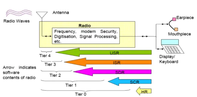
Radios can be classified accordingly to their capabilities:
Hardware Radio (HR): : The system cannot be changed via software;
Software-Controlled Radio (SCR): : Control functionality implemented in software, but change of attributes such as modulation and frequency band cannot be done without changing hardware;
Software-Defined Radio (SDR): : Capable of covering wide frequency range and of execut-ing software to provide variety of modulation techniques, wide-band or narrow-band operation, communications security functions and meet waveform performance require-ments of relevant legacy systems. System software should be capable of applying new or replacement modules for added functionality or bug fixes without reloading entire set of software. Separate antenna system followed by some wideband filtering, amplification, and down conversion prior to receive A/D-conversion. The transmission chain provides reverse function of D/A-conversion, analog up-conversion, filtering and amplification; Ideal Software Radio (ISR): : All of capabilities of software defined radio, but eliminates
analog amplification and heterodyne mixing prior to A/D-conversion and after D/A conversion;
Ultimate Software Radio (USR): : Ideal software radio in a chip, requires no external an-tenna and has no restrictions on operating frequency.
Software Defined Radio is further classified into three categories: • Reconfigurable Radio, based on FPGA technology only.
• Programmable Radio, based on a hybrid architecture DSP/FPGA • Fully Software Radio, based on General Purpose Processor
In our work we adopt fully software-radio approach employing Ettus USRP platform and RTL2832U devices.
Following tho approach a radio for SDR is associated to a PC of which it exploits the com-putational power, while it acts as a front-end. The front-end is responsible for sampling the
Figure 2.1: Classification of software radio devices
signal, executing a down-convertion from the RF to an Intermediate Frequency (IF) and con-verting the signal into digital information using an ADC. Clearly it is also possible to execute transmissions providing I-Q samples to the front-end that it will convert into a signal using a DAC and then will transmit at the RF.
SDR devices are programmable in the sense that are able to receive commands from a PC such as working parameters like the central frequency to tune, the sampling frequency etc. thanks to the FPGA technology and DSPs that substitute ASICs.
Since this kind of units are programmable, it is pretty easy to configure or update them without the need to manage hardware modules.
2.3
SCA standard
Since the panorama of SDR solution is quite wide [3], USA decided to start a project called Join Tactical Radio System (JTRD) to standardize the implementation of SDR solutions. The aim of the project was to standardize the distributed system architecture in order to facilitate portability of components and waveforms from a physical device to another regard-less of the diversity of the hardware platforms used by the different members of the group JTRD.
The result of this operation is the Software Communications Architecture (SCA) [4] which nowadays is a standard de facto for military applications. SCA is a distribute system
ar-chitecture that permits to deploy different components on different processing elements and to make them communicate through a middleware that, according to the specification, is CORBA. For specialized processors such as DSPs and FPGAs there exist several adapters that allow the communications with CORBA components.
The SCA objective is to ”establish an implementation-independent framework with baseline requirements for the development of software for Software Defined Radio”. It provides some constraints regarding the interfaces and structures of the software to promote reusability of code. The Core Framework is composed by four set of interfaces (Base Application Interfaces, Base Device Interfaces, Framework Control Interfaces and Framework Services Interfaces) and distinguishes between software components that require to access hardware resources (SCA devices) and software that does not require hardware resources (software only) referred as services.
Non-CORBA capable elements must use adapters that provide a translation between non-CORBA-capable components or devices and non-CORBA-capable Resources.
Figure 2.2: Operating Environment and relation with the Application Environment Profile
Application Components may need to access operating system resources but with some restrictions specified by the SCA Application Environment Profile. This environment is based on the POSIX specification which is a standard de facto and with some extensions is able to manage also real time applications.
The SCA specifies also the interface for some kind of components that are essentially a software abstraction of a physical hardware (Devices) and allow some particular kind of operations like capacity operations. A logical device implements one of the Base Device Interfaces. The most diffused version of the standard is actually the 2.2.2 although current version released by JTRD is 4.0.
Figure 2.3: SCA Architecture Layer
2.3.1 CORBA
The Common Object Request Broker Architecture is a middleware for communication be-tween remote objects by using the RPC mechanism. By introducing CORBA in SCA it is possible to realize different components handled by different processes, possibly residing on different machines with different architectures, communicate each other by exchanging messages without carying of the types implementation, the endian format, the address (by implementing the location transparency), and many other aspects of a connection that makes usually non trivial the exchanging of information in real time with different systems [5]. CORBA acts as a middleware because favor the inter-process communication without the programmer has to care about how the communication happens and the protocols involved. It is advised by SCA specification although it introduces an important overhead in the com-munication between components. This overhead is mainly due to the fact that CORBA exploits the TCP/IP protocol for communicating and has the necessity to make several type conversion, but, on the other hand, it has a large diffusion and maturity on almost all plat-forms with GPP and there exist several adapters for non fully supported platplat-forms.
The overhead introduced by CORBA is not linear but depend strongly from the packet length [6]. By increasing the length of the packet, the effect of the middleware overhead is mitigated and performances approach to those of the pure TCP/IP [7].
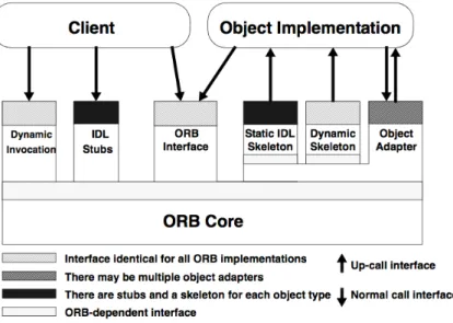
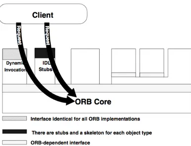
Since SCA uses CORBA, the learning of this architecture could be not easy and would require several months. To obviate to this inconvenient, some tools have been developed to facilitate the learning and utilization of SCA by letting the tool handling the CORBA connection and generating the XML files, while the programmer can focus on higher level task such as the development of the algorithm inside components. CORBA allows clients to send requests to objects implementations [8] by using the Dynamic Invocation interface or an IDL Stub which are a Object Reference.
Figure 2.4: CORBA client-object interaction
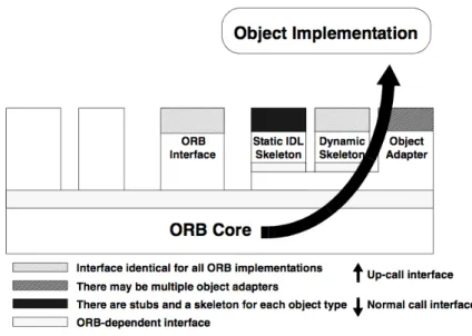
The ORB locates the right implementation of the interface which contains the method invoked by the client. The implementations are kept int the Implementation Repository. The client must know the type of the object on which is performing operations and the method to call.
The Object Implementation may choose which Object Adapter to use according to the service required. An Object Implementation provides the code for the objects methods, but clients have no knowledge of the implementation of the object.
In SCA CORBA provides also the Naming Service, the Log Service and the Event Service. Event channels allow the asynchronous communication between many producers and many consumers. Since this is an important source of delay, implementations of CORBA on a Network On Chip are under investigation [9].
Figure 2.5: Client performs a method invocation on a remote object through a remote reference
2.3.2 OSSIE
OSSIE, which has reached the release 0.8.2, is a SCA-compliant framework that stands at the basis of Redhawk. It is a project voted to research and education and includes an Integrated Development Environment based on Eclipse IDE, a waveform builder called WaveDash, a Core Framework based on SCA architecture and a collection of pre-built components. OSSIE project has now been discontinued in favor of Redhawk which utilizes many of its libraries and tools and presents a similar Graphic User Interface. OSSIE provides a graphical debugger for testing waveforms called ALF that helps the programmer to develop its own programs by means to some tools such as FFT, I-Q diagram, etc or to connect several blocks together.
Within OSSIE IDE it is possible to create new components or utilize those pre-built in the Core Framework, and deploy them into a node, that is a set of devices capable of managing streams of data like a General Purpose Processor or physical devices. Pre-defined node allo-cates a General Purpose Processor which is able to run the majority of waveforms.
The IDE allows the programmer to add ports and properties to components and to automat-ically generate the template of code in which it is possible to insert user code and contains the signature of the most used functions.
As Redhawk, OSSIE supports several programming languages such as C++ and Python. Since it has been discontinued, bugs will no more be fixed and developers strongly recom-mend to adopt the successor Redhawk.
Figure 2.6: The object receives a method invocation
However it remains the basic development tool in SCA world, often used in less recent releases.
Differences with Redhawk
Redhaw, as OSSIE evolution, presents several innovations and improvements.
First of all, the project management has become easier thanks to the tool-generated stereo-type of the code that does not overwrite previously user code. The Redhawk IDE allows the user to add ports, properties and implementations at any time of the development phase of the component, without any loss of the code.
Redhawk enhances also the waveform management. Now the programmer can use the mouse to link components, set or read their properties, move them along the waveform diagram, start and stop them singularly and connect them to a device in a way that is much more user friendly.
The developer has now the possibility to monitor in real-time many parameters of the stream of data that is flowing across component links through Stream Related Information, a struc-ture containing information related to the data stream like the sampling period or the type of data. Furthermore a SRI listener has been added to monitor data streams in real-time and allowing to adjust component properties. SRI are also used to communicate to other components the nature of the data stream, namely if it contains scalar or complex values, removing the need of a couple of ports to handle complex streams of data. Now complex streams contains I and Q samples interleaved and can be received using just one port. The programmer must pay attention to the nature of the stream if it is required by the
applica-Figure 2.7: CORBA middleware in SCA
tion.
It is now possible to plot graphics more easily in real-time just by clicking on ports, either for real or complex streams of data. New kinds of plots are now available like the waterfall and the oscilloscope and it is possible to monitor port statistics.
2.3.3 GNU Radio
SCA standard is not the only solution for SDR applications. Another solution coming from Open Source Community is GNU Radio, which is a toolkit that provides a development environment to develop waveforms and its components. It is based on C++ components connected through a Python interface. The performance of this framework is about 25 times faster in latency and 5 times lighter in computational load [10] wrt OSSIE, one of the most popular SCA implementations. This values are affected by the absence of a middleware and may vary according to the number of components that form the waveform.
This choice emphasizes the performance against the portability of the code that is one of the main issues in military applications since it is required to be able to move waveforms from
a device to another or to be compatible with newer devices. This could be an important limitation in case a developer wants to realize a waveform with a parallel architecture. GNU Radio suite of components provides to the developer a wide range of built-in components such as filters, channel codes, synchronization elements, equalizer, demodulators, vocoders, decoders, and others that allow to run several waveforms immediately after the installation [11]. It presents a GUI similar to Simulink and the possibility to use built in components or to create new ones.
GNU Radio is Open Source and has a large community of active developers that realized versions of this program for all major operating systems, including MS Windows and Mac OS X.
It provides a huge suite of signal processing libraries and supports a wide range of SDR devices, especially NI Ettus platforms. Probably it is the most used development tool by researchers and radio amateurs.
GNU Radio offers also the possibility to customize existing components or to create new ones and to share code with the community.
Redhawk
3.1
Redhawk Core Framework
Redhawk, as described here [12], is a Software Defined Radio framework which provides several tools for the development of software radio applications. Redhawk provides an IDE (Integrated Development Environment) which is useful for the realization of components that, combined together, can generate a waveform.
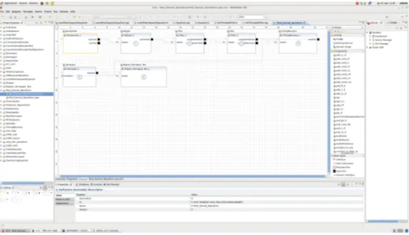
Redhawk derives from OSSIE project and is SCA compatible. Every component realized by using Redhawk should be portable to any other SCA compliant tool. It is very flexible since comes with a powerful code generator that masks the underlying middleware CORBA to the programmer and is suitable for didactic purposes due to its simplicity and the possibility to learn practically the signal processing. Some powerful tools are included within the IDE, such as an oscilloscope and a spectrum analyzer through which it is possible to monitor in real-time waveform conditions and adjust properties consequently.
3.2
IDE
Redhawk IDE is derived directly from Eclipse [13] and it’s easy to use for who is accustomed to program in C++ and Java since it presents and interface where the programmer can browse all her projects, open several file containing code, writing code with real-time syntax checking and compile. It also provides a Sandbox, a tool which offers the possibility to try components in customized waveforms very quickly, speeding up the production. The connection between components can be managed using the XML code manipulated through the text editor or through the graphical user interface of the program, by a simple drag and drop of the connection between ports. The IDE offers also the possibility to debug the code,
to start and stop nodes, to manage waveforms and a library of components.
The default layout of the IDE presents a left side panel listing all the project belonging to the user workspace. By clicking on them it is possible to inspect their content, open code files and add or remove contents. By right clicking on a project a menu appears: the user is allowed to compile code, delete all implementations and perform some other operations like cut, copy and paste.
On the bottom of the screen, a resizable panel occupy a third of the screen and its aim is to show the console where all compiling operation results are shown and where executables can print their log to communicate messages to the user. Also the Domain Manager and the Device Manager exploit this tool to show messages to the user. This panel has also some tabs that are used to show component’s properties, errors and the spectrum analyzer or the oscilloscope of Redhawk.
On top of the window there’s a menu bar that includes all the functionalities of the program, while on the right there is a list of all components installed in the computer and the controller of the Sandbox and the Domain Manager.
In the center there’s a space for the text editor for handling open files or to host the chalkboard or the editor of waveforms.
3.3
Sandbox
Redhawk Sandbox is a powerful tool of the IDE that allows the programmer to develop and test components very rapidly without the necessity to deploy a waveform to test components. To use the Sandbox, expand the Sandbox menu on the right panel and double click on the Chalkboard application.
The Sandbox presents a whiteboard in the central panel of the scene and a list of all available components that can be deployed. The user drags and drops components from the list to the board and they will be expanded to form a box. Each box contains inside the name of the component and has on the edge some squares that represent ports. Ports on the left are input ports and are of white color, while those on the right are output ports and are black. ports can be connected together through a wire. In order to connect two ports together, they the must be of the same type. Simply draw a wire with drag and drop from the square that represent an output port to the square that stands for an input port.
Components can be configured with some parameters. To configure a component simply click on it and a menu will appear on the bottom panel of the application. You can set up all the properties allowed for the component that are listed in a table.
Figure 3.1: Redhawk IDE and the Sandbox
To start a component right click on it and then Start or, alternatively, from the chalkboard menu right click on the component icon and then Start. To start all components right click on the Chalkboard and start all components. The same procedure applies when you want to stop a component. You can selectively stop a single component or the entire waveform. When you’re done you can click on the Chalkboard and then release all components.
The Sandbox tool is comfortable for fast prototyping waveforms or testing single components, but presents a general slow down of the performances. If a single component crashes all the others can continue working and it is possible to correct bugs and deploy it again.
The Sandbox can also be used and configured from terminal, and requires the knowledge of Python language.
The Sandbox offers to the user the possibility to save prototyped waveforms into the files system for further retrieve although it is not possible yet to load stored waveform in the Sandbox.
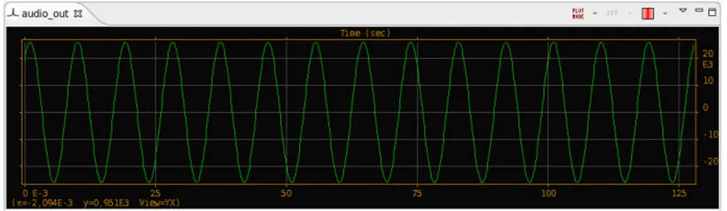
When components are running there is the possibility to monitor the current status of each one simply by clicking on it and inspecting its properties. If you right-click on a port you can select to show port statistics from the menu. Port statistics are useful to monitor the stream of data flowing through the component and its amount. For output ports it is also possible to plot the oscilloscope and the spectrum analyzer.
Figure 3.2: Oscilloscope tab
3.4
Components
Redhawk components present a similar schema which we’re going to introduce.
Typically they present two kinds of ports: input ports and output ports. There exist also input/output ports but we will not talk about them. Input ports of a component are con-nected to output ports of another component, to form a chain.
Components can be developed using different programming languages. Redhawk supports C++, Java and Python as developing languages. Since we require a high level of perfor-mances, we chose to utilize C++, that is a compiled language and doesn’t run in a virtual machine. By using C++ we have also a finer control over data, at the cost of the need to manually manage memory allocation and deallocation.
Components can be placed into the Sandbox and connected together to form a waveform, then can be configured by modifying by hand certain parameters called properties. Once all the settings have been performed, the waveform can be started. It is possible to monitor the output port of each component and plot the data in the time and frequency domain. It is also possible to adjust parameters and connections in real time, without restarting the Sandbox. Therefore this solution of using components is the easiest for developing and testing. Usually, after design, they’re placed into a waveform stored in a SAD file from which they can always be retrieved.
Component life cycle is expressed explicitly in the SCA standard, and here we will summarize the basic usage and development. To create a new components a user has to click on File → new → SCA Component Project. The system will prompt several windows to the user that will have to specify at least the name of the component and its implementing language. The system will generate automatically a skeleton of the project, including SPD file. Using the graphical editor, the programmer can add ports and properties. Once the file has been completed, Eclipse generates automatically all the implementation of the component. In the implementation file (i.e. FilterComparison.cpp) the user will find a brief manual of
basic programming rules: /* * B a s i c f u n c t i o n a l i t y : The s e r v i c e f u n c t i o n is c a l l e d by the s e r v i c e T h r e a d o b j e c t ( of t y p e P r o c e s s T h r e a d ) . T h i s c a l l h a p p e n s i m m e d i a t e l y a f t e r the p r e v i o u s c a l l if the r e t u r n v a l u e for the p r e v i o u s c a l l was N O R M A L .
If the r e t u r n v a l u e for the p r e v i o u s c a l l was NOOP , t h e n the s e r v i c e T h r e a d w a i t s
an a m o u n t of t i m e d e f i n e d in the s e r v i c e T h r e a d ’ s c o n s t r u c t o r .
SRI :
To c r e a t e a S t r e a m S R I object , use the f o l l o w i n g c o d e : std :: s t r i n g s t r e a m _ i d = " t e s t S t r e a m ";
B U L K I O :: S t r e a m S R I sri = b u l k i o :: sri :: c r e a t e ( s t r e a m _ i d ) ;
T i m e :
To c r e a t e a P r e c i s i o n U T C T i m e object , use the f o l l o w i n g c o d e : B U L K I O :: P r e c i s i o n U T C T i m e t s t a m p = b u l k i o :: t i m e :: u t i l s :: now ()
;
P o r t s :
D a t a is p a s s e d to the s e r v i c e F u n c t i o n t h r o u g h the g e t P a c k e t c a l l ( B U L K I O o n l y ) .
The d a t a T r a n s f e r c l a s s is a port - s p e c i f i c class , so e a c h p o r t i m p l e m e n t i n g the
B U L K I O i n t e r f a c e w i l l h a v e its own type - s p e c i f i c d a t a T r a n s f e r .
The a r g u m e n t to the g e t P a c k e t f u n c t i o n is a f l o a t i n g p o i n t n u m b e r t h a t s p e c i f i e s the t i m e to w a i t in s e c o n d s . A z e r o v a l u e is non - b l o c k i n g . A n e g a t i v e v a l u e is b l o c k i n g . C o n s t a n t s h a v e b e e n d e f i n e d for t h e s e values , b u l k i o :: C o n s t :: B L O C K I N G and b u l k i o :: C o n s t :: N O N _ B L O C K I N G . E a c h r e c e i v e d d a t a T r a n s f e r is o w n e d by s e r v i c e F u n c t i o n and * M U S T * be e x p l i c i t l y d e a l l o c a t e d .
To s e n d d a t a u s i n g a B U L K I O i n t e r f a c e , a c o n v e n i e n c e i n t e r f a c e has b e e n a d d e d
t h a t t a k e s a std :: v e c t o r as the d a t a i n p u t
N O T E : If you h a v e a B U L K I O d a t a S D D S port , you m u s t m a n u a l l y c a l l " port - > u p d a t e S t a t s () " to u p d a t e the p o r t s t a t i s t i c s w h e n
a p p r o p r i a t e .
E x a m p l e :
// t h i s e x a m p l e a s s u m e s t h a t the c o m p o n e n t has two p o r t s :
// A p r o v i d e s ( i n p u t ) p o r t of t y p e b u l k i o :: I n S h o r t P o r t c a l l e d
s h o r t _ i n
// A u s e s ( o u t p u t ) p o r t of t y p e b u l k i o :: O u t F l o a t P o r t c a l l e d
f l o a t _ o u t
// The m a p p i n g b e t w e e n the p o r t and the c l a s s is f o u n d // in the c o m p o n e n t b a s e c l a s s h e a d e r f i l e b u l k i o :: I n S h o r t P o r t :: d a t a T r a n s f e r * tmp = s h o r t _ i n - > g e t P a c k e t ( b u l k i o :: C o n s t :: B L O C K I N G ) ; if ( not tmp ) { // No d a t a is a v a i l a b l e r e t u r n N O O P ; } std :: vector < float > o u t p u t D a t a ; o u t p u t D a t a . r e s i z e ( tmp - > d a t a B u f f e r . s i z e () ) ; for ( u n s i g n e d int i =0; i < tmp - > d a t a B u f f e r . s i z e () ; i ++) { o u t p u t D a t a [ i ] = ( f l o a t ) tmp - > d a t a B u f f e r [ i ]; } // N O T E : You m u s t m a k e at l e a s t one v a l i d p u s h S R I c a l l if ( tmp - > s r i C h a n g e d ) { f l o a t _ o u t - > p u s h S R I ( tmp - > SRI ) ; } f l o a t _ o u t - > p u s h P a c k e t ( o u t p u t D a t a , tmp - > T , tmp - > EOS , tmp - > s t r e a m I D ) ; d e l e t e tmp ; // I M P O R T A N T : M U S T R E L E A S E THE R E C E I V E D D A T A B L O C K r e t u r n N O R M A L ;
If w o r k i n g w i t h c o m p l e x d a t a ( i . e . , the " m o d e " on the SRI is set to t r u e ) , the std :: v e c t o r p a s s e d f r o m / to B u l k I O can be t y p e c a s t to / f r o m
b u l k i o :: I n S h o r t P o r t :: d a t a T r a n s f e r * tmp = myInput - > g e t P a c k e t ( b u l k i o :: C o n s t :: B L O C K I N G ) ;
std :: vector < std :: complex < short > >* i n t e r m e d i a t e = ( std :: vector < std :: complex < short > >*) &( tmp - > d a t a B u f f e r ) ;
// do w o r k h e r e
std :: vector < short >* o u t p u t = ( std :: vector < short >*) i n t e r m e d i a t e ; m y O u t p u t - > p u s h P a c k e t (* output , tmp - > T , tmp - > EOS , tmp - > s t r e a m I D ) ;
I n t e r a c t i o n s w i t h non - B U L K I O p o r t s are l e f t up to the c o m p o n e n t d e v e l o p e r ’ s d i s c r e t i o n
P r o p e r t i e s :
P r o p e r t i e s are a c c e s s e d d i r e c t l y as m e m b e r v a r i a b l e s . For example , if the
p r o p e r t y n a m e is " b a u d R a t e " , it may be a c c e s s e d w i t h i n m e m b e r f u n c t i o n s as
" b a u d R a t e ". U n n a m e d p r o p e r t i e s are g i v e n a g e n e r a t e d n a m e of the f o r m
" p r o p _ n " , w h e r e " n " is the o r d i n a l n u m b e r of the p r o p e r t y in the PRF f i l e .
P r o p e r t y t y p e s are m a p p e d to the n e a r e s t C ++ type , ( e . g . " s t r i n g " b e c o m e s
" std :: s t r i n g ") . All g e n e r a t e d p r o p e r t i e s are d e c l a r e d in the b a s e c l a s s
( F i l t e r C o m p a r i s o n _ b a s e ) .
S i m p l e s e q u e n c e p r o p e r t i e s are m a p p e d to " std :: v e c t o r " of the s i m p l e t y p e .
S t r u c t p r o p e r t i e s , if used , are m a p p e d to C ++ s t r u c t s d e f i n e d in the g e n e r a t e d f i l e " s t r u c t _ p r o p s . h ". F i e l d n a m e s are t a k e n f r o m the n a m e
in
the p r o p e r t i e s f i l e ; if no n a m e is given , a g e n e r a t e d n a m e of the f o r m
" f i e l d _ n " is used , w h e r e " n " is the o r d i n a l n u m b e r of the f i e l d .
E x a m p l e :
// T h i s e x a m p l e m a k e s use of the f o l l o w i n g P r o p e r t i e s :
// - A f l o a t v a l u e c a l l e d s c a l e V a l u e
// - A b o o l e a n c a l l e d s c a l e I n p u t
d a t a O u t [ i ] = d a t a I n [ i ] * s c a l e V a l u e ; } e l s e { d a t a O u t [ i ] = d a t a I n [ i ]; } A c a l l b a c k m e t h o d can be a s s o c i a t e d w i t h a p r o p e r t y so t h a t the m e t h o d is c a l l e d e a c h t i m e the p r o p e r t y v a l u e c h a n g e s . T h i s is d o n e by c a l l i n g
s e t P r o p e r t y C h a n g e L i s t e n e r ( < p r o p e r t y name > , this , & F i l t e r C o m p a r i s o n _ i :: < c a l l b a c k method >) in the c o n s t r u c t o r . E x a m p l e : // T h i s e x a m p l e m a k e s use of the f o l l o w i n g P r o p e r t i e s : // - A f l o a t v a l u e c a l l e d s c a l e V a l u e // Add to F i l t e r C o m p a r i s o n . cpp F i l t e r C o m p a r i s o n _ i :: F i l t e r C o m p a r i s o n _ i ( c o n s t c h a r * uuid , c o n s t c h a r * l a b e l ) : F i l t e r C o m p a r i s o n _ b a s e ( uuid , l a b e l ) { s e t P r o p e r t y C h a n g e L i s t e n e r (" s c a l e V a l u e " , this , & F i l t e r C o m p a r i s o n _ i :: s c a l e C h a n g e d ) ; } v o i d F i l t e r C o m p a r i s o n _ i :: s c a l e C h a n g e d ( c o n s t std :: s t r i n g & id ) { std :: c o u t < < " s c a l e C h a n g e d s c a l e V a l u e " < < s c a l e V a l u e < < std :: e n d l ; } // Add to F i l t e r C o m p a r i s o n . h v o i d s c a l e C h a n g e d ( c o n s t std :: s t r i n g &) ; */
In these suggestions there are some important aspects of Redhwak framework. First of all Stream Related Information. These informations are collected in a structure that is passed along the waveform between component’s ports. SRI have several fields, some of which are very important for signal processing; one of the most important is for sure the fieldmode, which expresses the nature of the stream of data. A value of this field equal to 0 indicates that the
stream contains real values, 1 that the stream is complex. As stated in these suggestions, complex streams are sent as an interleaved stream of real and imaginary parts, compatible with the complex type of C/C++ languages.
SRI contains also time information like the sampling period called xdelta, useful when we need to sample or filter data. Last useful field is the streamID, that contains a string that identifies the stream, in case we’re working with multiple streams.
Another important aspect suggested in this brief guide is the typical behavior of the compo-nent. Usually it starts with a call to a port to get a packet. A packet is a structure containing a burst of data, a timestamp, a SRI structure and a flag. The data type contained in the packet must be one of the supported CORBA data types and is stored as astd::vectorof the same type of the port. It’s forbidden to connect two ports that are not of the same type. Once data has been received, it can be processed using whatever algorithm the programmer retains necessary. After processing, the Stream Related Information must be forwarded to the adjacent component. If some elaborations have changed the values of the structure, the
sriChanged flag must be set. Then processed data can be sent down the stream for further
elaboration.
The usage of std::vector structure is recommended since it easiers life to the programmer while classical C/C++ pointers are more error prone. Anyway there’s fully compatibility between the two types since it is possible to convert astd::vector into an array with a little trick:
std::vector<float> m y V e c t o r;
// do s o m e w o r k w i t h m y V e c t o r
f l o a t * m y A r r a y = &m y V e c t o r[ 0 ] ;
This technique is useful since all data information comes from ports that treat data as
std::vector and are sent still as std::vector, but for elaboration sometimes C arrays can be
more comfortable.
Auto generated code derives from the base implementation of the component which is respon-sible of implementing basic functionality of the life cycle, ports and properties as variables of the class. In order to access or modify a property it’s sufficient to refer it through its name as a common variable. It is also possible to register the component to listen for property modifications, in case it is necessary to perform special operations when a change occurs. Once the component has been developed, drag and drop it on to the library icon in the right panel called Target SDR to install it into the$SDRROOT folder.
3.5
Devices and Device Manager
According to SCA, Redhawk permits to develop a special kind of components: the devices. Devices have the same structure of common components but also have special methods to allocate and deallocate capacity. Devices may, in fact, require resources that the hosting operating system must provide through system resources or physical devices. The allocation of a device fails if it is not possible to satisfy its requirements. Redhawk basic installation comes with a predefined device, the GPP.
Devices can be grouped to form nodes. These may contain different hardware devices and a GPP.
Devices are handled by a special module of Redhawk called Device Manager. The aim of the Device Manager is to parse Node’s Device Configuration Descriptor
3.6
Domain Manager
The Domain Manager is a program whose interface allows the control of the entire system Domain.
The Domain Manager keeps track of a File Manager, a set of Device Managers and Appli-cation Factories. It also manage user’s waveforms. The Domain Manager is also responsible of facilitating the interaction of the user with the system parts like Devices, Services and Application capabilities.
Applications (better known as waveforms ) are descripted in a SAD file which is a XML file containing a list of all components used and how they’re are linked together. It may also specify how Devices are connected to components and their allocation properties.
In SAD files it is also expressed the start order of each component of the waveform.
The Domain Manager is responsible of the life cycles of the nodes. Nodes can be created by the user to host devices. The system has a default node which includes a GPP, but it is possible to create a customized one.
To create a new node:
• From the file menu click on new and then SCA Node Project. The editor will prompt you a window where it will be possible to customize the node.
• To add devices to the node simply drag and drop them from the list on the right. • It is possible to change some properties of the devices by clicking on the property tab.
• Once all configuration have been completed, save the file and drag and drop the Node project in the Target SDR library.
• In order to launch a node, right click on the Target SDR library and then launch. A popup window will ask you which node to launch.
• Select the node you want to launch and then ok.
If everything will work correctly, the node will be listed on top right and showed as con-nected.
It is possible to inspected a running node to monitor some parameters like ports and SRI, plot some data with the spectrum analyzer or the oscilloscope and allocate or deallocate a front-end tuner.
To allocate a front-end tuner you need to right-click on the device of the node you want to customize and then allocate. You can specify the central frequency, the bandwidth, the sampling rate and tolerances. If parameters are corrected, the tuner will be allocated. The user can connect an allocated front-end tuner to a waveform or some Sandbox components.
3.7
Installation
Redhawk installation is not as easy as one could expect. Several problems often arises during the installation process that requires some IT skills in order to be solved. On official Redhawk website a list of the steps necessary to accomplish this task can be found. Anyway we decided to add some additional information and suggestions that could help in this preliminary phase. It is strongly recommended to install Redhawk framework on a CentOS 6.5 machine since older versions can have some compatibility issues and other distributions of Linux, like Ubuntu or Fedora, may present some incompatibilities with some libraries that are not easy to solve for a non very skilled programmer and require time.
Other operating systems different from Linux are discouraged although many libraries are available also for Mac OS X thanks to programs like Mac Ports and Homebrew. Anyway the framework is not mature enough to allow a easy porting on other Operating Systems. Before installing the framework, it is required to install a series of packages. These can be easily managed through the packet manager Yum. Many packages are available only after adding the Extra packages for Enterprise Linux repository to Yum. We discourage to install packages through source code because this will make the removal or upgrade harder.
Once all packages have been installed, it is time to install the framework. It comes in a tar archive that contains all the packages required. After the installation process, the user must
add herself to the Redhawk group for permissions.
In order to install the Eclipse IDE, Java must be installed and configured on the machine. At the end of the installation process, the user must configure CORBA omniORB. During the framework usage, CORBA often does not release the name of the Domain Manager and in order to start it again it is required to restart omniNames and omniEvents. We provide a simple script that should be launched before initiating a session and when the Domain Manager stops responding and has to be terminated:
# !/ bin / sh
/s b i n/s e r v i c e o m n i E v e n t s s t o p
/s b i n/s e r v i c e o m n i N a m e s s t o p
rm -f /var/log/o m n i O R B/* /var/lib/o m n i E v e n t s/* /s b i n/s e r v i c e o m n i N a m e s s t a r t
/s b i n/s e r v i c e o m n i E v e n t s s t a r t
3.7.1 UHD driver
In order to be able to use the UHD USRP device produced by Ettus research [14] it is necessary to install appropriate driver for the device.
Drivers can be downloaded from the official website but require some steps to accomplish all the task required. In particular there are not rpm packges available for CentOS distribution so it is necessary to install them using the source code. Before this operation, anyway, some dependencies must be satisfied. In particular:
1. Download the driver archive from here https://github.com/EttusResearch/UHD/tags 2. Follow these instruction to install drivers http://files.ettus.com/manual/page build guide.
html paying particular attention to dependencies
3. Execute the command ldconfig at the end of the process installation.
4. Setup Udev for USB as specified here http://files.ettus.com/manual/page transport.html# transport usb
5. Check the correctness of the installation by connecting the USRP to the USB port and executing uhd find devices command in the terminal
6. If the command is not found, consider exporting the path of the folder in which the program is installed.
7. If required, edit the file/etc/ld.so.confand add the path of the library to the file
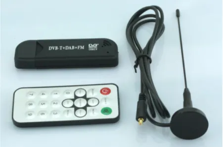
3.7.2 RTL
RTL is a USB wideband receiver for DVB-T and FM and is a useful tool for learning SDR through direct experience. In order to use it with Redhawk it is necessary to install appro-priate drivers from Osmocom website [15] and follow the installation procedure.
Figure 3.3: RTL USB DVT-B receiver
Once the driver has been installed, it is necessary to download also the RTLTcpSource component for Redhawk. To use the USB dongle with Redhawk
1. Plug the RTL dongle into a USB port
2. Open the terminal of your operating system and execute rtl tcp program 3. Open Redhawk and launch the Sandbox
4. Place the RTLTcpSource in the Chalkboard and the required components to form a waveform.
5. Configure properties of the components adequately.
6. Right click on the Chalkboard icon and then start. The RTLTcpSource component will connect to the rtl tcp program and will start to receive data.
Components
In this chapter many components realized for this work will be introduced and explained in their main functions and aim. The strategy adopted on many of them is to include classes into Redhawk components in order to be able to export the code easily instead of embedding the code together with the management of the data. To facilitate this aspect and to avoid loss of performance we decided in many circumstances to instantiate/garbage objects when components are started and stopped. Many objects have a sort of status or memory, so it would be a bad choice to allow the user to change certain properties dynamically.
4.1
Convolutional encoder and Viterbi decoder
Convolutional Encoder is a component whose aim is to encode data accordingly to a schema provided by a generator. The generator is a set of masks that is used in encoding and it’s provided by the user through the GUI of Redhawk as a property of the component.
As dual component, the Viterbi Decoder is able to decode a string of bits encoded by the Convolutional Encoder, provided the same parameters of the generator. The Decoder is able to execute also the depuncturing operation on its own according to the mask set by the user or work in conjunction with the Depuncturer component.
To work correctly, the strings of bits must have a minimum length that depends on the parameters used to configure the component.
Convolutional codes are used in telecommunications as error correction codes to make digital communications more reliable and have been employed in many fields, from Voyager program to many satellites. Viterbi algorithm [16] tracks the state of a stochastic process with a recursive method that is optimum [17]. The decoder is based on shift registers and a trellis structure divided in segments that form different branches along which are disposed received
Figure 4.1: Convolutional Encoder with generator (7, 5)
data. A reading of the constructed path from the end to the beginning gives us the original sequence of bits that were encoded with a convolutional code.
4.2
Mapper and Demapper for QAM and PSK
One of the most common operation that must be performed by SDR applications is the mapping of strings of bits into symbols and viceversa. We realized a couple of components that are able to execute PSK and QAM mapping and demapping.
Both components include a class for handling PSK and QAM mapping and demapping. The components can be configured through some properties to execute a mapping/demapping mode or another and some parameters related to the choice such as constellation size. The component itself instantiates the class required and, upon the reception of new data, calls the correct method of the class. In case of mapping the Mapper transforms a sequence of bits in symbols. A symbol is a complex number that represents one or more bits according to the size of the constellation and mode. The symbols are then forwarded towards other components and then transmitted by the radio front-end.
Demapping operation, on contrary, takes a sequence of one or more symbols as input and transforms it into a sequence of bits.
The components are configured at the moment of the start and can be reconfigured only if the user stops them.
The QAM mapper is configured providing it the size of the constellation (the number of symbols); it will build a matrix, stored in memory, that will contain the IQ samples to
send. Symbols will be then associated to strings of bits. Adjacent elements of the matrix maps strings that differ for only one bit accordingly to the Grey code in order to minimize errors. The association of strings of bits to the symbols is performed by realizing first a table containing all the Grey coded values of the numbers from 0 to the size of the matrix - 1.
N16= 0 1 2 3 7 6 5 4 8 9 10 11 15 14 13 12 (4.1)
Figure 4.2: 16 QAM map
Number Grey Coded Value 0 0000 1 0001 2 0011 3 0010 4 0110 5 0111 6 0101 7 0100 8 1100 9 1101 10 1111 11 1110 12 1010 13 1011 14 1001 15 1000
When the match is found, say the i-th entry, the (complex) value that corresponds to the i-th element in the symbol table is returned. Entries are not numbered sequentially from left to right, from top to down, but rather as a snake from top left to down right, to put adjacent codes close to each other.
Q16= 0000 0001 0011 0010 0100 0101 0111 0110 1100 1101 1111 1110 1000 1001 1011 1010 (4.2)
PSK mapping and demapping is obtained by creating a table containing all the symbols with their real and complex parts. Parallel to this table, another table is used for Grey encoding of numbers. Both tables have the same size. When you need to encode a bit string, first look for a match in the table of codes and take the index of the match. Then use the symbol at the same index in the symbol table.
Grey code is generated as follows:
/* *
* @ b r i e f C o d i f y a s y m b o l by u s i n g the G r e y c o d e *
* G i v e n a bit string , the f u n c t i o n l o o k s for the i n d e x
* of the s y m b o l t h a t m a p s the s e q u e n c e by u s i n g the G r e y c o d e . * The i n d e x is e v a l u a t e d as seq ^ ( seq > > 1 )
*
* @ p a r a m seq s e q u e n c e of bit to map *
* @ r e t u r n the m a p p e d v a l u e in G r e y c o d e */
int qam::g r e y C o d e(u n s i g n e d c h a r seq) {
r e t u r n (seq ^ (seq> >1) ) ; }
/* *
* @ b r i e f D e c o d e a s y m b o l by u s i n g the G r e y c o d e *
* G i v e n the i n d e x of a symbol , the f u n c t i o n l o o k s for the s t r i n g * of b i t s t h a t is m a p p e d by the s y m b o l by u s i n g the G r e y c o d e . * The d e c o d i n g o p e r a t i o n is p e r f o r m e d as f o l l o w :
* for e a c h bit of the c o d e d1 ... dn c o u n t the n u m b e r of b i t s * t h a t are set on the l e f t of the i - th bit ( so d1 ... dk w i t h * k < i ) . If the c o u n t is odd , f l i p the bit . R e p e a t u n t i l all the * b i t s are a n a l y z e d . * * @ p a r a m c o d e the s e q u e n c e of bit to d e m a p * * @ r e t u r n the s e q u e n c e of bit d e m a p p e d */ u n s i g n e d c h a r qam::g r e y D e c o d e(u n s i g n e d c h a r c o d e) { u n s i g n e d c h a r r e s u l t = 0x00; for (u n s i g n e d int i = 0; i < N _ b i t; i++) { u n s i g n e d c h a r tmp = c o d e > > (i+1) ; bitset<8 > set(tmp) ; b o o l bit = (c o d e > > i) & 0x01; if (set.c o u n t() % 2 != 0) r e s u l t |= !bit < < i; e l s e r e s u l t |= bit < < i; } r e t u r n r e s u l t; }
4.3
Spreader and Despreader
Spread spectrum communications like UMTS have nowadays a large use in commercial ap-plications. This system is based on the composition of two different signals, one that carries the information and one at high frequency that adds some redundancy to the signal and is orthogonal to the codes used for other signals.
Figure 4.3: Spreading of a signal s(t) using the signal c(t)
This makes it possible to transmit different signal s(t) (represented as a NRZ function, unitary amplitude and duration T) in the same channel without interference.
s(t) =X
i
aip(t − i T ) (4.3)
Each spreading signal is composed by a sequence of chips at a high rate wrt the data signal.
c(t) =X
l
clq(t − l Tc) (4.4)
The resulting signal is the multiplication of the two signals. The ratio between the rate of the two signals is the spreading factor M .
M = Rb Rc (4.5) xss(t) = s(t) · c(t) (4.6) By defining γl= abl Mc · cl xss(t) = X i ai h X l clq(t − l Tc) i p(t − i T ) =X l γlq(t − l Tc) (4.7)
Since we’re going to treat bits that can be assimilated to a signal modulated as OOK, the operation of spreading is performed by xoring data bits with the Hadamard codes ai⊕ clThe
Hadamard codes are taken from a Hadamard table that is built in memory by the component. The size of the Hadamard table depends on the configuration of the respective property of the component and is connected to the spreading factor that the user want to realize.
−6 −4 −2 0 2 4 6 −0.2 0 0.2 0.4 0.6 0.8 1 1.2 f S(f) S s(f) S xss(f)
Figure 4.4: Spectrum of the signal (red) and the spreaded signal (blue) with spreading factor equal to 5
Hadamard Codes Hadamard Codes, also known as Walsh Codes or Walsh-Hadamard
Codes, are used to distinguish communications channels. Codewords are used to identify users inside cells in CDMA communications and have the property to be orthogonal. Unless two users adopt the same codeword, the transmission of a user will appear like noise to the other users in the cell. Codewords are composed by a binary alphabet. The code matrix can be built using a generator matrix that is replicated according to a schema. To generate the Hadamard table, starting from the smallest table of 1x1 elements, it’s sufficient to append copies of the matrix on the right and on the bottom while the copy on the bottom right must be changed in sign. H1 = (1) (4.8) H2 = 1 1 1 −1 ! = H1 H1 H1 −H1 ! (4.9) H3= 1 1 1 1 1 −1 1 −1 1 1 −1 −1 1 −1 −1 1 = H2 H2 H2 −H2 ! (4.10)
In general: Hi= Hi−1 Hi−1 Hi−1 −Hi−1 ! (4.11)
4.4
Puncturer and Depuncturer
Puncturer Depuncturer is a component that is used in conjunction with encoding and decod-ing operations for convolutional codes to add and remove bits from a strdecod-ing accorddecod-ing to a mask provided by the user. The Puncturer and the Depuncturer utilize the mask to remove the specified bits from a sequence or to add zeroes in certain positions to enlarge a sequence.
Figure 4.5: Encoder with rate 2/3
This can be used to get fractional rates starting from a rate of 1/2 and to reduce the number of bits that is necessary to send over the channel, with a consequent increment of the error probability. This components can be built as an embedded function of the encoder or decoder for convolutional codes but we decided to make also a specific component edition to be more flexible when building waveforms.
4.5
FFT/iFFT
Transformations from time domain to frequency domain and viceversa are common operations in SDR waveforms. It can be necessary for filtering or some analysis and requires a lot of computational power. Luckily this issue has been faced several times in the past and an existing good solution can be represented by FFTW library, which is a performant library that is able to perform FFT and inverse FFT. This library allows the programmer to execute the FFT with an arbitrary resolution and to exploit the parallelism to increase the performances of the system. Although it’s possible to manage all the operations manually by writing a component that performs all the transform computations, we chose to integrate the FFTW solution as is in this component without any modification because we repute it very optimized.
To check the goodness of the component, we can send a signal to the FFT and then apply the inverse transform to check if the result is the same as the input. Obviously it is also possible to check the result of the FFT block by looking at the spectrum analyzer offered by Redhawk IDE or comparing the signal observed through the oscilloscope before and after FFT/iFFT.
Since the FFTW library is robust and well made, specifying the compiler to use multiple threads to compute the transform will help to make computations faster.
4.6
Converters
This class of component is similar to that provided by the Core Framework of Redhawk but is able to handle only short and float values. It can convert input data from real to complex and can transform float data into short and viceversa.
There exists some components of this family such as ShortToFloat, Float to Short and Real to Complex, which perform the cast specified by the name. When a cast from float to short is required, the conversion takes into account the representation interval available for the short type. In fact float input data (real or complex) are first scaled and then multi-plied by the maximum integer representable in a short value (215− 1 = 32767).
Scaling factor is evaluated as the maximum value that the float input can assume. User may specify in a property the maximum value to use for scaling in order to maintain a dynamic of values that occupies all the possible values offered by the short type.
4.7
Rate Adapter
Rate Adapter is a component that acts as a buffer to adapt the rate of symbols from a component to another that have different speeds. In particular the adapter varies the length of the streams of symbols that are sent from the output port. The size can be enlarged or reduced according to the necessity. It has an internal memory buffer to store temporary samples before packetizing them. The buffer is implemented as a queue due to its frequent size change and implements the FIFO policy. If the buffer contains enough elements, a block of size specified by the user is output from the port, otherwise data is retained until it reaches the volume required. The front of the queue is continually shifted, while new samples are enqueued at the end. This component may affect a lot the performance of the waveform since it can increase or decrease rates and anyway introduces a delay due to the processing of enqueueing/dequeueing.
Its application could be necessary when some components require a input rate that is constant or has a specified number of symbols, while the source of data is not constant and thus it’s necessary to apply a buffer that maintain the rate constant at the desired value. This version of the buffer works on symbols which carry a different number of bits according to the mapping used, but its bit version implementation is straight forward.
4.8
Random Generator
The Random Generator is a component whose aim is to produce a pseudo random sequence of bits of arbitrary length. In order to generate the sequence of bits, the generator requires to know the seed to adopt in the generation process and the size of the strings of bits generated. To not overwhelm following components the Random Generator waits a certain amount of time (actually 1 s) before sending another string.
If the rate of generation of bits exceed the waiting time, the rate obtained will be less than expected. The generated bits are represented as short values since CORBA does not provide a boolean type to map C++bool type.
4.9
Write and Forward
This component has been realized in order to monitor and record the traffic that flows through a branch of the waveform. In fact it is able to read and store data that pass through it in a location specified by the user and then push data towards the following component. It is completely transparent to data but since it requires to perform some disk IO operations it could reduce performance of high data rate. Anyway with modern SSD technology this issue should be alleviated and shouldn’t be noticed by the end user. In case performances were considered essential and there were no margin for delays, we recommend to not insert this component in the middle of critical paths of data since may slow down the effective data rate.
4.10
Scrambler
Scrambler component, also called randomizer, is used to invert the normal ordering of bits in order to exploit some code property and for cryptography. The variation may be used also when a sequence of bits is repeated frequently. The scrambler is structured as a series of registers that are used to memorize a pattern, initialized with a seed. At every iteration bits are shifted between register components. According to a mask, bits are also summed each
other. The user may choose to use all the registers or only a part of them, starting from the lowest ones (least significant bits). If used, a scrambler component must be placed either in the transmitter and in the receiver, both initialized with the same seed and with the same mask.
Altering the normal sequence of bit by scrambling helps to reduce errors on streams of data and makes the initial sequence of bit appearing as random noise to an observer along the channel.
4.10.1 Scrambler for symbols
We realized a version of the scrambler oriented to PSK symbols. This version is a slight modification of the scrambler for bits, since the internal structure remains the same. This component is able to map the internal status of the scrambler into a symbol, according to the size of the PSK constellation specified as a property.
The obtained symbol, which is simply the mapping of the first bits of the scrambler in the constellation, is then multiplied with the input symbol of the component. The waveform programmer must be careful when using the component not to use symbols that map strings of bits longer than the internal register size.
Figure 4.6: Scrambler with 12 registers and generator 1000001010011.
Since register elements depend on each other, this component does not beneficiate signifi-cantly from a parallel architecture.
4.11
Block Interleaver
According to some military standards, we realized a component that is able to execute the interleaving of the input in blocks.
Interleaving operation is performed on streams of data to change the natural ordering of bits. This helps to reduce the impact of noise on transmissions. Data is usually transferred in bursts and it may happen that one or more of them are corrupted due to noise in the channel. Some error-correcting algorithms are usually applied but they have some limits on
the maximum number of flipped bits they’re able to detect and correct. Repositioning of bits creates a more uniform distribution of errors and therefore it’s easier to recover a damaged burst of data.
Input bit strings are picked up in sequence and are put in a matrix according to a schema provided by the user which spreads the input in all the rows of the matrix. Bits are then mixed again inside the matrix, typically copying the loaded matrix into another, inverting the previous ordering. Once data is received by the receiver, bits are treated in inverse order and repositioned correctly in the matrix. Then bits are extracted from the matrix following the same schema used to insert them.
The matrix in which bits are inserted can be represented as an array made by a sequence of rows. Input bits are inserted every k position (load factor), filling remaining gaps with zeroes. Then the matrix is copied into the second matrix. This time bits are fetched every n (fetch factor) positions from the input array and are inserted sequentially into the output matrix.
Figure 4.7: Example of block interleaver with load factor of 3 and fetch of 9.
In order to deinterleave the sequence, the same procedure is applied to the sequence, but with k0 = n and n0 = k.
4.12
Convolutional Interleaver
The Convolutional Interleaver is a kind of interleaver that makes use of a series of shift registers of different length to memorize bits coming from the input data stream. The register number is chosen by the user and must be the same for the Interleaver and the Deinterleaver. Their length is different and starts from the unitary registers and increase according to a step provided by the user as a property in the Interleaver, while in the Deinterleaver, on the contrary, the register length starts from longest down to the unitary register with decrements equal to the the increment used in the Interleaver. Bits are inserted in the first element of
each shift register of the Interleaver. The schema used to insert bits in the registers may vary according to user specifications, but the default is sequentially. Then registers are shifted of a position and last bits of each register are output. Then a new series of bits can be inserted in the Interleaver. The process continues until all the input bits haven’t been inserted and all the bits in the longest register have been output. Zeroes are inserted when no more input bits are available and we need to shift the registers. Registers are initialized with zeroes.
Figure 4.8: Convolutional interleaver with 4 shift registers and increments of 2.
The Deinterleaver acts in a dual way. Received bits are inserted in the registers in their arrival order and then elements are shifted of a position. Output is picked up according to the same schema used for inserting bits in the Interleaver (default sequentially), starting from the longest register. The process terminates once all bits have been inserted into registers, shifted and extracted. The output will have a set of zeroes preceding the sent data. Since the schema used is known a priori, the number of zeroes added is known and it is possible to extract just the desired data from the output.
Figure 4.9: Convolutional deinterleaver with 4 shift registers and decrements of 2.
The number of zeroes is given by the length of the longest register times the number of the registers, minus the first column that is equal to the number of registers.