Alma Mater Studiorum
· Università di Bologna
SCUOLA DI SCIENZECorso di Laurea in Informatica
On the Hidden Subgroup Problem
as a Pivot in Quantum
Complexity Theory
Relatore:
Chiar.mo Prof.
UGO DAL LAGO
Presentata da:
ANDREA COLLEDAN
Sessione I
Contents
Introduction 3
A Top-down Approach . . . 4
1 The Hidden Subgroup Problem 6 1.1 A Mathematical Approach . . . 6
1.2 A Computational Approach . . . 9
1.2.1 Group Encoding . . . 9
1.2.2 Function Encoding . . . 11
1.2.3 The HSP Functional . . . 13
2 The Importance of the HSP 14 2.1 Reducibility and Complexity . . . 14
2.2 Interesting Problems . . . 19
2.2.1 Simon’s Problem . . . 20
2.2.2 The Discrete Logarithm Problem . . . 21
3 An Introduction to Quantum Computing 26 3.1 Quantum Systems . . . 26
3.1.1 The State of a System . . . 27
3.1.2 The Evolution of a System . . . 29
3.1.3 Composite Systems . . . 31
3.1.4 Entanglement . . . 35
3.2 Quantum Computing . . . 37
3.2.1 Quantum Gates . . . 38
3.2.2 Quantum Circuits . . . 44
4 A Quantum Solution for Abelian Groups 50 4.1 Preliminaries . . . 50
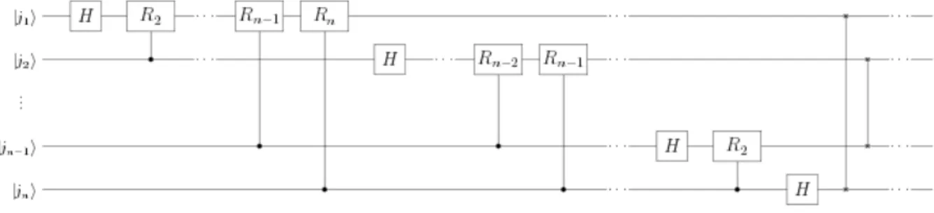
4.1.1 The Quantum Fourier Transform . . . 50
4.1.2 Converting Classical Circuits . . . 55
4.3 Representation Theory . . . 62
4.4 General Abelian Case . . . 63
4.4.1 More Representation Theory . . . 64
4.4.2 The QFT on Abelian Groups . . . 67
4.4.3 The Algorithm . . . 69
Conclusions 74 Integer Factorization . . . 74
Non-Abelian Groups . . . 75
Introduction
It is in the mid-1990s that some of the most notorious quantum algorithms make their first appearance in the research community. In 1995, Peter Shor presents two game-changing quantum algorithms: one solves the integer factorization problem, the other the discrete logarithm problem. Both do so in polynomial time, i.e. exponentially faster than any of the best known classical algorithms [12]. One year later, Lov Kumar Grover presents a quantum algorithm for searching databases that is quadratically faster than any possible classical algorithm for the same purpose [6].
Shor’s work, in particular, deals effectively with two well-known intractable computa-tional problems and hints at the possibility of using quantum computers to tackle more of those problems that, although very valuable, cannot be reasonably solved by classical machines. However, because quantum algorithms are significantly harder than classical algorithms to design, breakthroughs such as Shor’s are very rare to come by. This is where the idea of finding a single abstract problem that generalizes a larger class of com-putationally hard problems starts being of great interest and this is where the hidden
subgroup problem comes into play.
It is not uncommon, in computer science, for a particular problem to gain impor-tance and notoriety not thanks to its inherent practical value, but rather for being an exceptional representative of a larger class of attractive problems. This is the case with the hidden subgroup problem (also labeled HSP), an abstract problem of group theory that happens to be an excellent generalization of exactly those problems that quantum computers can solve exponentially faster than their classical counterparts.
In its purest form, the hidden subgroup problem consist in, given a group, determin-ing which ones of its subgroups give birth to cosets accorddetermin-ing to a certain function f , which can be consulted like an oracle. The abstract nature of this problem allows it to generalize numerous aspects of, among others, order finding and period finding problems [11]. Furthermore, many cases of the HSP are already known to allow efficient quantum solutions, a fact that makes the HSP a perfect choice of representative for many of the intractable problems that we are interested in.
A Top-down Approach
Most of the literature on the hidden subgroup problem approaches the topic in a
bottom-up fashion. That is, first the principles that rule quantum mechanics and quantum
computing are introduced, then they are used to give solutions to a number of problems. Finally, these problems are generalized to the HSP.
In this thesis, we attempt to partially reverse this approach by giving a top-down perspective on the role of the HSP in quantum complexity theory. First we present the problem in its pure, mathematical form. Next, we give a computational definition of the same problem and we show how an algorithm that solves it can be used to solve other, more interesting problems. After that, we introduce those concepts of quantum computing that are strictly necessary to understand some of the quantum algorithms that efficiently solve the HSP on specific group families. Lastly, we discuss these algorithms.
More in detail, this thesis is structured as follows:
• In Chapter 1 we discuss the hidden subgroup problem per se. First, we introduce the essential group-theoretical concepts necessary to understand the problem at hand, of which we give a formal, mathematical definition. We then shift our attention to the computational details of the HSP, to define more rigorously what it means to compute a solution to it. It is in this chapter that we define the concept of HSP functional.
• In Chapter 2 we introduce some essential concepts of complexity theory and re-ducibility. We then use these concepts to discuss the pivotal role of the HSP in the context of quantum complexity theory. We also go out of our way to concretely show how two significant computational problems can be reduced to the HSP. • Those readers who are only acquainted with classical computing may perceive the
subject of quantum computation as equally fascinating and daunting. In prepara-tion for the quantum algorithms that are shown in Chapter 4, Chapter 3 presents a brief introduction on the principles of quantum mechanics and their application to computer science.
• Lastly, in Chapter 4 we examine how the quantum Fourier transform can be used to implement quantum algorithms that efficiently solve the HSP on specific types of groups, namely Abelian groups. As a consequence, this algorithms allow us to efficiently solve the problems that we introduced in Chapter 2.
The idea behind this order of exposition is that of allowing the target reader, i.e. the computer scientist with little to no knowledge of things quantum, to get acquainted with the hidden subgroup problem and to be convinced of the importance of its role in complexity theory, without necessarily having to deal with the intricacies of quantum computing. However, we do hope that this thesis will stimulate the reader into further pursuing the study of this fascinating subject.
Chapter 1
The Hidden Subgroup Problem
1.1
A Mathematical Approach
The first step in our top-down approach is, of course, to provide a definition of the problem at hand and to get acquainted with it. To do so, it is first advisable to review a number of concepts of group theory, starting with the very definition of group.
Definition 1.1.1 (Group). Let G be a set and ◦ a binary operation on the elements of
G. The tuple (G, ◦) constitutes a group when:
• G is closed under ◦, i.e. ∀g1, g2 ∈ G : g1◦ g2 ∈ G.
• There exists an identity element e∈ G such that ∀g ∈ G : g ◦ e = g = e ◦ g. • For every element g ∈ G there exists an inverse element, i.e. an element g−1 ∈ G
such that g◦ g−1 = e = g−1◦ g.
Example 1.1.1: A simple example of a group is (Z, +), the set of all integers under
addition. This is a group because the sum of any two integers is itself an integer, there exists an identity element (0 ∈ Z) and for all n ∈ Z, there exists (−n) ∈ Z such that
n + (−n) = n − n = 0.
Example 1.1.2: On the other hand, the tuple (Z, ×), although similar, does not
con-stitute a group: Z is closed under multiplication and there exists an identity (1 ∈ Z), but in general the inverse of an n∈ Z (i.e. 1/n) does not belong to Z.
From now on we will often refer to a group of the form (G, ◦) as simply G, specifying the underlying operation only when strictly necessary. Furthermore, we will work mostly with additive and multiplicative groups (groups in which the operation is addition or multiplication, respectively). When working with additive groups we will write g1 + g2
instead of g1 ◦ g2 and −g instead of g−1. Similarly, when working with multiplicative
groups, we will write g1· g2 (or simply g1g2) and g−1.
If a subset of the elements of G exhibits itself group structure under G’s operation, then such a subset is called a subgroup of G.
Definition 1.1.2 (Subgroup). Let H be a subset of the elements of a group (G, ◦). H
is a subgroup of G (and we write H ≤ G) when:
• H is closed under G’s operation, i.e. ∀h1, h2 ∈ H : h1◦ h2 ∈ H.
• The identity element of G is in H.
• For every element h∈ H, the inverse element h−1 is also in H.
Example 1.1.3: Let us consider the group G = (Z, +) from the previous example. The
set H = {2n|n ∈ Z} of even integers is a subgroup of G, as it is closed under addition (the sum of any two even numbers is even), contains the identity element 0 and the inverse of an even number is even as well.
Example 1.1.4: On the other hand, the subset of odd integersK = {2n+1|n ∈ Z} does
not form a group (because 0 /∈ K) and neither does the subset Z+ of positive integers
(no positive number has a positive inverse).
Both groups and subgroups can be described in terms of a subset of their elements, from which we can obtain all the other elements via the group operation. Such a subset is called a generating set for the group.
Definition 1.1.3 (Generating set of a group). LetG be a group and S = {s1, s2, . . . , sn}
a subset of its elements. We denote by ⟨S⟩ the smallest subgroup of G that contains all the elements of S. We say that S is a generating set for G when ⟨S⟩ = G.
Example 1.1.5: Consider G and H from the previous example. We have that G = ⟨1⟩,
as we can easily express any integer n with|n| sums of 1 or −1. It is also evident, by its very definition, that H = ⟨2⟩.
By applying ◦ between elements of H and generic elements of G we obtain elements that do not necessarily belong toH. In particular, if we apply ◦ between all the elements of H and one element of G, we obtain what is called a coset.
Definition 1.1.4 (Coset). Let G be a group and let H ≤ G. For every g ∈ G we can
• gH = {g ◦ h|h ∈ H}, or the left coset of H with respect to g. • Hg = {h ◦ g|h ∈ H}, or the right coset of H with respect to g.
For h∈ H, we have hH = H = Hh, so H is one of its own cosets. In general, however, the left and right cosets are different. When the left and right cosets coincide for all
g ∈ G then H is said to be a normal subgroup. Of course, this is always the case when
G’s operation is commutative. In this case, G is said to be Abelian.
Definition 1.1.5 (Abelian group). A group G is an Abelian group when ∀g1, g2 ∈ G :
g1◦ g2 = g2◦ g1. That is, when ◦ is commutative.
Example 1.1.6: Consider again G and H from Example 1.1.3. First, we note that G
is Abelian, as addition is commutative. Next, we see that H only has one coset, that is 1H = H1 = {2n + 1|n ∈ Z}, the set of odd numbers.
We now have enough background to introduce the crucial concept of coset-separating
function, which lies at the very heart of the hidden subgroup problem.
Definition 1.1.6 (Coset-separating function). Let G be a group and let H ≤ G. Let
f :G → S be a function from the elements of G to finite-length binary strings. We say that f separates cosets for H when:
∀g1, g2 ∈ G : f(g1) = f (g2) ⇐⇒ g1H = g2H.
In other words, f separates cosets when it is constant on the individual cosets of H and different between different cosets. Essentially, f identifies the cosets ofH by labeling them with distinct strings of bits. We are now ready to introduce the hidden subgroup problem:
Definition 1.1.7 (Hidden Subgroup Problem). LetG be a group and H ≤ G an unknown
subgroup. Let f : G → S be a coset-separating function for H. The Hidden Subgroup
Problem (HSP) consists in finding a generating set for H by using the information
provided by f .
In practice, we will only work with finite groups. Consider a family {GN}N∈I, where
I ⊆ N is a set of indices. The members of such a family are groups with similar operations, whose elements come from the same superset. What distinguishes them is their order. Namely, for all GN ∈ {GN}N∈I we want |GN| to be a function of N.
Example 1.1.7: All the groups inside{ZN}N∈N have elements in the non-negative
inte-gers Z∗. Each ZN ∈ {ZN}N∈N has addition modulo N as group operation and has order
We therefore define a variant of the HSP, generalized to families of groups:
Definition 1.1.8 (Parametrized HSP). Let{GN}N∈I be a family of groups. The HSP on
{GN}N∈I consists in, given N and a function fN that separates cosets for someHN ≤ GN,
finding a generating set for HN by only using information obtained from evaluations of
fN.
1.2 A Computational Approach
Up to this point we have built a mathematical definition of the HSP. For our purposes, however, we need a more rigorous definition of what it means to solve the HSP on a certain input. Namely, we want to define a functional for a group family {GN}N∈I,
which takes a specific N and some representation of a coset-separating function f as inputs and outputs some representation of a generating set for the desired subgroup. Essentially, we want to give a computational definition of the parametrized HSP that we defined in the previous section. To do so, we first need a way to effectively encode groups and functions.
1.2.1
Group Encoding
Suppose we are working with a group family{GN}N∈I. Consider the total disjoint union
G of the elements of this family:
G = ⊎
N∈I
GN.
This new setG consists of ordered couples of the form (g, N), such that g ∈ GN. Consider
now a function ρ :G → S × N such that ρ is an injection from G to the pairs of finite-length binary strings and integers. We call such ρ an encoding function for the group family {GN}N∈I. We want ρ(g, N ) = (bg, N ), so that every element g of every possible
group in the group family can be represented as a binary string bg. From now on, we
will often refer to such bg as ρ(g, N ) or simply ρ(g), ignoring N in the process.
Definition 1.2.1 (Polylogarithmic function). A function f : N → N is said to be
polylogarithmic if it consists of a polynomial in the logarithm of the input. That is, f is
of the form:
f (x) = a0+ a1⌊log x⌋ + a2⌊log x⌋2+· · · + ak⌊log x⌋k.
Definition 1.2.2 (Length-predictable function). Let{AN}N∈Ibe a family of sets and let
A be their total disjoint union. A function ρ : A → S is said to be length-predictable (LP) if there exists f :N → N such that, for all (a, N) ∈ A, we have |ρ(a, N)| = f(N). If f is a polylogarithmic function, then we say that ρ is polylogarithmically length-predictable (PLP).
If an encoding ρ is LP for some f : N → N, then we can identify the elements of a group GN with strings of exactly f (N ) bits. We now attempt to provide encoding
functions for some of the group families we will work with.
Groups of Binary Strings Consider the group family {(BN,⊕)}
N∈N, whose groups
consist of the binary strings of length N under addition modulo 2.
Lemma 1.2.1. For all N , the set BN of binary strings of length N forms a group of
order 2N under addition modulo 2.
Proof. The set of binary strings of length N has exactly 2N elements. For all b
1, b2 ∈ BN,
b1 ⊕ b2 is also a binary string of length N . Furthermore, there exists in BN the identity
element e = 0N such that for all b∈ BN, b⊕ 0N = b. Lastly, every element b∈ BN is its
own inverse, as b⊕ b = 0N.
In this case our encoding function ρ is trivially the identity function, asBN is already
a subset ofS (its elements are fixed-length binary strings). It is obvious that the output of ρ grows linearly with N . As such, ρ is LP for f (N ) = N .
Cyclic Additive Groups Before we say anything about the encoding of cyclic additive groups, let us provide a definition:
Definition 1.2.3 (Cyclic group). A groupG is said to be cyclic if there exists an element
g ∈ G such that ⟨g⟩ = G. That is, G can be generated by a single element, known as the
generator of the group.
Consider now {ZN}N∈N, the family of cyclic additive groups of integers modulo N .
In this case, and for all N , our ρ is the “identity” function ρ(z, N ) = (binN(z), N ), where
binN(x) is the zero-padded binary representation of an integer x≤ N. Note that for all
such x, binN(x) is always a string of⌊log2N⌋ + 1 bits. Being the elements of ZN exactly
the integers from 0 to N − 1, we can say that this ρ is PLP.
Finite Abelian Groups Consider {GN}N∈I, a family of generic Abelian groups. Let
us introduce the concept of direct sum of groups:
Definition 1.2.4 (Direct sum of groups). Let G1 andG2 be two groups. The direct sum
of G1 and G2 is the group G of pairs (g1, g2), where g1 ∈ G1 and g2 ∈ G2. We write
G = G1⊕ G2.
Of course, the direct sum of any two Abelian groups is also Abelian. We have the following result [8]:
Theorem 1.2.1. Every finite Abelian group GN is isomorphic to a direct sum of cyclic
additive groups. That is, there exist N1, N2, . . . , Nk such that:
GN ∼=ZN1 ⊕ ZN2 ⊕ · · · ⊕ ZNk.
As a result, we have that every element g ∈ GN can be represented by a k-tuple
(z1, z2, . . . , zk) such that zi ∈ ZNi for every i = 1 . . . k. At this point, we can define ρ′
on ZN1 ⊕ · · · ⊕ ZNk as the concatenation of the outputs of the cyclic additive ρ on the
elements of the tuple:
ρ′((z1, z2, . . . , zk), N ) = (binN1(z1)∥ . . . ∥ binNk(zk), N ).
Of course, Ni is smaller than N for every i = 1 . . . k. Furthermore, we have an upper
bound on k as well:
Lemma 1.2.2. Let{GN}N∈Ibe a family of groups an let g :{GN}N∈I → N be a function
such that, for all GN ∈ {GN}N∈I, g(N ) = |GN|. Then if GN ∼= ZN1 ⊕ ZN2 ⊕ · · · ⊕ ZNk
we have that
k ≤ ⌈log2g(N )⌉.
Proof. IfGN and ZN1⊕ ZN2⊕ · · · ⊕ ZNk are isomorphic, then necessarily g(N ) =|GN| =
|ZN1 ⊕ ZN2 ⊕ · · · ⊕ ZNk| = N1N2· · · Nk. Of course, k is greatest (we have the greatest
number of factors) when N1, N2, . . . , Nk are the prime factors of g(N ). For every k, the
smallest number with k prime factors is 2k. Therefore, any number n cannot have more
prime factors than the smallest 2k ≥ n, i.e. 2⌈log2n⌉, which has exactly ⌈log
2n⌉ prime
factors. It follows that g(N ) has at most ⌈log2g(N )⌉ prime factors.
As a result, our encoding ρ′ is surely LP for some f ∈ O(log N(log g(N))). Moreover, if g is a polynomial then f ∈ O(log2N ) and ρ′ is PLP.
Properties of the encoding One last property that we expect from our encoding functions is that it must be possible to efficiently compute common group operations on the binary representations they produce. In the case of groups of integers, these operations are addition, multiplication and exponentiation, and we know that polytime algorithms exist that can compute them on the binary representations produced by ρ [7]. Furthermore, we require that ρ allow efficient inversion.
1.2.2
Function Encoding
Once we have ρ that encodes the elements ofGN as finite-length binary strings, we have
all the means necessary to turn any coset-separating function as given in Definition 1.1.6 into an equivalent coset-separating function that operates on binary strings. To define such a function, we first need to introduce the concept of boolean circuit.
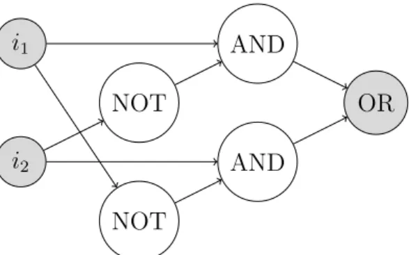
i1 i2 NOT NOT AND AND OR
Figure 1.1: A simple example of a boolean circuit that computes addi-tion modulo 2 (i.e. the exclusive or operaaddi-tion).
Definition 1.2.5 (Boolean circuit). A boolean circuit C of n inputs and m outputs is
a directed acyclic graph in which:
• There are n input nodes, labeled i1, i2, . . . , in, which have an in-degree of 0.
• The remaining nodes are labeled with either AND, OR or NOT and have in-degrees of 2 ( AND, OR) or 1 ( NOT).
• Among the non-input nodes, there are m output nodes, which have an out-degree of 0.
Definition 1.2.6 (Function of a circuit). Let C be a boolean circuit of inputs i1, i2, . . . , in
and outputs o1, o2, . . . , om. We say that C computes a function fC :Bn→ Bm defined as
fC(x1, x2, . . . , xn) = (y1, y2, . . . , ym),
where y1, y2, . . . , ym are the boolean values produced by o1, o2, . . . , on when the input nodes
are assigned values x1, x2, . . . , xn.
Note that once we know how to represent a boolean circuit as a directed acyclic graph, it is also easy to encode it as a string. All we need to do is store every node, along with a label, and every edge as a couple of nodes. The size of such an encoding is fairly easy to estimate. Suppose we are given a boolean circuit as a graph GC = (V, E):
• Nodes: For each each node in V we need to store an identifier and a label. We can uniquely identify the nodes of GC using the integers from 0 to |V | − 1.
As a result, each identifier requires O(log|V |) bits to be stored. The label, on the other hand, requires constant space. The nodes can thus be stored using
• Edges: For each of the|E| = O(|V |2) edges, we need to store the identifiers of the
nodes involved. Each identifier requires O(log|V |) bits to be stored, so the total number of bits required is O(|V |2)· O(log |V |) = O(|V |2log|V |).
Putting the two things together, we have that a a boolean circuit C with n gates can be represented by a string of O(n2log n) + O(n log n) = O(n2log n) bits. We will refer
to such a string as ⌈C⌉.
Now that we have the notion of a circuit that computes a function from binary strings to binary strings, we can bring in our ρ to define the notion of coset-separating circuit.
Definition 1.2.7 (Coset-separating circuit). Let GN be a group in a group family
{GN}N∈I and let HN ≤ GN. Also, let ρ : G → S × N be a LP encoding function
for some f : N → N. We say that a boolean circuit C separates cosets for HN with
respect to ρ if C computes a function fC : Bf (N ) → Bm (for some big enough m), such
that:
∀g1, g2 ∈ GN : fC(ρ(g1, N )) = fC(ρ(g2, N )) ⇐⇒ g1HN = g2HN.
We can then encode the graph of such coset-separating circuit C as a binary string
⌈C⌉, which can serve as an effective way to pass a coset-separating function as the input
of our functional.
1.2.3
The HSP Functional
We conclude this chapter by giving a formal definition of the HSP functional, which will serve as the foundation of our discussion on the computational importance of the HSP.
Definition 1.2.8 (HSP functional). Let{GN}N∈Ibe a family of groups and let ρ : G → S
be a suitable encoding function for such family, LP for some function f : N → N. A
function F : S × S → S is said to be a HSP functional for {GN}N∈N and ρ if and
only if on inputs bin(N ) and ⌈C⌉, where C is a boolean circuit that separates cosets for some HN ≤ GN with respect to ρ, F returns ρ(h1, N )∥ρ(h2, N )∥ . . . ∥ρ(hm, N ), such that
{h1, h2, . . . , hm} is a generating set for HN.
Let us try and decode this definition. In informal terms, what a HSP functional does is solve the HSP problem on all the members of a fixed group family with a valid encoding. For every input group GN (represented by N ) and coset-separating function f on it
(represented by the description of circuit C), such a functional outputs a concatenation of the elements that generate the subgroup HN ≤ GN identified by f .
Chapter 2
The Importance of the HSP
In the previous chapter we presented the hidden subgroup problem in its purest form and we defined, through the HSP functional, what it means to compute a solution to one of its instances. It is now time to address why the HSP is such a significant problem from a computer science perspective.
2.1
Reducibility and Complexity
A fundamental concept in theoretical computer science is that of reduction between problems. A problem is said to be reducible to a second problem when an algorithm that solves the latter can be employed as a subroutine inside an algorithm that solves the former.
On a practical level, reductions are particularly useful when some properties about either one of the problems (usually the one that is reduced) are unknown. A typical example of such property is computability: if we know that a certain function f can be computed (i.e. an algorithm exists that computes it), then by reducing any other function g to f we prove that g can be computed as well, as in the process we must have shown that an algorithm for g can be built using the algorithm for f .
That said, the formal definition we provide is in some measure stricter than the in-formal description of the above paragraphs, but it is particularly well-suited for our purposes.
Definition 2.1.1 (Reducibility). Let fA and fB be two functions. We say that fA is
reducible to fB (and we write fA ≤ fB) if and only if there exist two computable functions
pushA and pullA such that:
That is, if xA is an input for fA, pushA converts xA into an input for fB (“pushes”
xA into fB). This new input is such that pullA can convert fB’s output into the correct
output for fA (pullA “pulls” the desired results out of fB). Let us examine an informal
(and imaginative) case of reducibility:
Example 2.1.1: Imagine we know how to sort a list of integers, by ascending or
de-scending order. Imagine also, with a willing suspension of disbelief, that we want to find the smallest and greatest elements of a list, but we don’t know how. Specifically, we know how to compute
sort(list, order),
in which order can be asc or desc. This function returns a new list in which the elements of list are sorted accordingly. We want to find a way to compute
extreme(list, which),
where which can be either min or max. This function needs to return the small-est/greatest integer in list, depending on which. We find a way to compute extreme by reducing it to sort. In particular, we define:
pushextreme(list, which) = {
(list, asc) if which = min, (list, desc) if which = max.
If we run sort(pushextreme(list, which)) we get a sorted list in which the first element is the smallest integer if which = min, or the greatest integer if which = max. That being said, we define:
pullextreme(sortedList) = f irst(sortedList).
This way, the final output of pullextreme(sort(pushextreme(list, which))) is the smallest integer in list if which = min and the greatest one if which = max, which is exactly the behavior we expected from the definition of extreme. By reducing extreme to sort, we proved that the former is computable.
Reductions in complexity theory Another field in which reductions play a signifi-cant role is that of complexity theory, as we can often provide insights on the complexity of a function fA by reducing it to a second function fB of known complexity (or
vice-versa). In particular, if fA ≤ fB then we have proof that fA cannot be harder than fB
to compute (or conversely, that fB is at least as hard as fA).
Of course, to say so we must first impose some constraints on the complexity of pushA and pullA. Taken as it is, Definition 2.1.1 allows us to say, for example, that any function
fA is reducible to the identity function id, as by setting pushA = fA and pullA = id we
have id(id(fA(x))) = fA(x). Although correct, this reduction is devoid of any usefulness
Therefore, for fA ≤ fB to be a sensible reduction we impose not only that pushA ̸=
fA̸= pullA, as that would defeat the purpose of a reduction entirely, but also that these
functions be easier, or at least no harder than fBto compute. That is, the computational
complexity of pushA and pullA must be negligible within the structure of a reduction. Let us clarify what we mean by first providing a review of some basic concepts of complexity theory. Let M be a deterministic Turing machine. Assume we have these functions at our disposal:
• stepsM(x): the execution time of M on input x, i.e. the number of computational steps required by M to accept (or reject) x.
• cellsM(x): the space required by M on input x, i.e. the number of distinct cells
visited by M ’s head during its computation on x.
We use them to define the following time and space functions:
Definition 2.1.2 (Time and space functions). Let M be a deterministic Turing machine.
We define the following functions:
• timeM(n) = max{stepsM(x)| n = |x|},
• spaceM(n) = max{cellsM(x)| n = |x|}.
Which measure the worst-case number of steps (and cells, respectively) required by M to compute on an input of length n.
If M computes a certain function fM, then timeM and spaceM provide us with
infor-mation on the computational requirements (i.e. time and space resources needed) of fM
on inputs of a certain length.
With that in mind, we can now define precisely what we mean when we talk about the complexity of a function. More specifically, we can define complexity classes, for time and space both. If two different functions belong to the same complexity class, then we can expect their computational requirements to grow similarly with respect to the size of their inputs. In fact, what a complexity class tells us about its members is precisely
Definition 2.1.3 (FTIME and FSPACE classes). Let g : N → N be a function between
natural numbers. We define:
• FTIME(g) = {f : S → S | ∃M : f = fM, timeM ∈ O(g)},
• FSPACE(g) = {f : S → S | ∃M : f = fM, spaceM ∈ O(g)}.
Where M is a Turing machine. In other words, we say that f belongs to FTIME
(FSPACE) of g if a Turing machine M exists that computes f and whose timeM (spaceM)
function is O(g).
Therefore the complexity of a function is nothing more than the relationship between the size of its inputs and the computational resources needed to process them. For some specific choices of g, we obtain classes of particular interest. For example:
FP = ∪
c∈N
FTIME(nc).
FP constitutes the class of functions which run in polynomial time (their worst-case running time grows like a polynomial in the size of the input). Another important complexity class is:
FLOGSPACE = FSPACE(log).
FLOGSPACE is the class of functions whose space requirements grow logarithmically with the size of their input.
Let us return to reductions. Previously, we said that in the case of a reduction fA≤ fB
we wanted our pushAand pullA functions to be of negligible complexity. What we meant was that if fBbelongs to FTIME(g) for some g, we want the composition pullA◦fB◦pushA
to still belong to FTIME(g).
In the case of fB ∈ FP, this amounts to finding pushA, pullA ∈ FP, as FP is closed
under composition. As we will see in the following chapters, this is the case that most interests us. Because of that, we define the concept of polynomial-time reductions.
Definition 2.1.4 (Polynomial-time reducibility). Let fA and fB be two functions. We
say that fA is reducible to fB in polynomial time (and we write fA ≤p fB) if fA ≤ fB
We conclude this small digression on complexity by formally introducing the concept of circuit families that compute a function.
Definition 2.1.5 (Circuit family). Let g :N → N be a function. A g-size circuit family
is a sequence {CN}N∈N of circuits in which CN has N inputs and size |CN| ≤ g(N). A
function f :S → S is said to be in SIZE(g) if there exists a g-size circuit family {CN}N∈N
such that, for all x∈ {0, 1}N, we have f (x) = f CN(x).
Definition 2.1.6 (P-uniform circuit family). A circuit family {CN}N∈N is said to be
P-uniform if there exists a polynomial-time Turing machine that on input 1N outputs
CN.
We prove that there exists a strong link between functions in FP and P-uniform circuit families. To do so, we need to introduce the concept of oblivious Turing machine, which is a Turing machine whose head movements are fixed. More formally:
Definition 2.1.7 (Oblivious Turing machine). A Turing machine M is said to be
obliv-ious if the movements of its heads are fixed instead of being dictated by the machine’s
input. That is, M is oblivious if its transition function is of the form δ : Q×Γk→ Q×Γk.
Lemma 2.1.1. Let M be a Turing machine that runs in time O(g). An oblivious Turing
machine M′ exists that simulates M and runs in time O(g2)[1].
With these considerations in mind, we proceed to prove that every polynomial-time function can be computed by a P-uniform circuit family. Note that this is a modified version of a result given in [1] (Theorem 6.6):
Lemma 2.1.2. Let f : S → S be a function between binary strings. If f ∈ FP, then f
is computable by a P-uniform circuit family.
Proof. Let us show how, once we fix a generic n, we can build a circuit that computes f on inputs of size n. If f ∈ FP, then there exists a polynomial-time Turing machine M that computes f . By Lemma 2.1.1, there exists an oblivious Turing machine N that
simulates M with a quadratic slowdown. It follows that N also computes f in polynomial time. Now, let x ∈ {0, 1}n be an input for N . Define the transcript of N on x to be
the sequence m1, m2, . . . , mtimeN(n)of snapshots (current state and symbols read by each
head) of N ’s computation. We can encode each snapshot mi as a fixed-length binary
string. Furthermore, we can compute such string from: • The input x,
• The snapshots mi1, . . . , mik, where mij denotes the last step in which N ’s jth head
was in the same position as it is in the ith step. Note that since N is oblivious, these do not depend on the input.
Because these are a constant number of fixed-length strings, we can use a constant-sized circuit to compute mi from the previous snapshots. By composing timeN(n) such
circuits, we obtain a bigger circuit C that computes from x to N ’s final state, i.e. C computes f . Also note that since N is polytime, C is of size polynomial in n.
We now have enough material to actually start talking about the importance of the hidden subgroup problem. Although in its simplest form the HSP may appear to be nothing more than non-trivial, yet uninteresting problem of group theory, it is proven that a significant number of traditionally hard computational problems can be reduced efficiently to specific instances of the HSP. These include the simplest quantum problems (e.g. Deutsch-Jozsa and Simon’s problem), as well as some of the hardest classical problems, such as the integer factorization and discrete logarithm problems, or the graph isomorphism problem.
It follows that finding an efficient solution to the HSP – and for some specific types of groups such a solution exists – would entail having an efficient way to solve problems that have always been deemed intractable. Even more specifically, the HSP models well those computational problems for which quantum algorithms exist that are exponentially faster than their classical counterparts. This is the reason why this problem plays such a valuable role in quantum algorithmics.
For a function fAto be reducible to the HSP there must exist a group family{GN}N∈I,
an encoding function ρ and two functions pushA, pullA such that:
• pushA takes the same inputs as fA and returns an input of the form (bin(N ),⌈C⌉)
for the HSP functional on{GN}N∈I and ρ.
• pullAtakes as input the output ρ(x1)∥ . . . ∥ρ(xm) of the HSP functional on{GN}N∈I
and ρ and returns the output expected from fA.
2.2
Interesting Problems
The main goal of this chapter is to show how some of these hard problems can be reduced to the HSP. Namely, we first reduce Simon’s problem, a problem specifically devised to showcase the superiority of quantum algorithms. After that, we reduce a more complex and practical problem, i.e. the discrete logarithm problem.
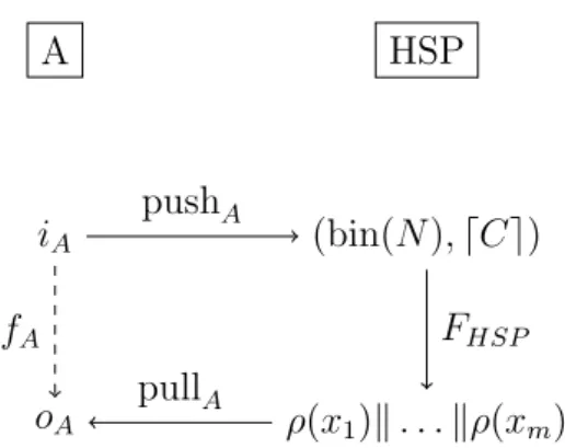
A HSP iA (bin(N ),⌈C⌉) oA ρ(x1)∥ . . . ∥ρ(xm) pushA FHSP pullA fA
Figure 2.1: A schematic representation of the reduction of a generic problem A to the HSP, where FHSP is the HSP functional as defined
in the previous chapter.
2.2.1
Simon’s Problem
Simon’s problem was conceived in 1994 by computer scientist Daniel R. Simon [13]. It is a problem of little practical value, explicitly designed to be hard for a classical computer to solve, but easy for a quantum computer to tackle.
Definition 2.2.1 (Simon’s Problem). Let f : Bn → Bn be a function such that there
exists some s∈ Bn for which the following property is satisfied:
∀x, y ∈ Bn: f (x) = f (y) ⇐⇒ (x = y ∨ x ⊕ s = y).
That is, f is the same when its arguments are the same or when they differ by summation modulo 2 with s. Simon’s Problem (SP) consists in, given f , finding s.
In computational terms, we can assume that SP takes as inputs ⌈CSP⌉, the
represen-tation of a circuit computing a suitable function fSP :BN → BN, and bin(N ), and that
it outputs s itself. The reduction of SP to the HSP is fairly straightforward [11]. Consider the family of binary string groups {(BN,⊕)}
N∈N. It is easy to prove that a
function f :BN → BN that satisfies Simon’s property is also a coset-separating function
onBN.
Lemma 2.2.1. Let f :BN → BN be a function from binary strings to binary strings. If
f satisfies Simon’s property for some s ∈ BN, then f is a coset separating function for
the subgroup {0, s} ≤ BN.
Proof. By definition, f (x) = f (y) if and only if x = y or x⊕ s = y. For all x ∈ BN, f is
the same on {x ⊕ 0, x ⊕ s} = x{0, s}, or the left coset of {0, s} with respect to x, and distinct for different choices of x. That is, f separates cosets for {0, s} ≤ BN.
It is also worth noticing that{0, s} = ⟨s⟩. With these results in mind, we choose the identity function as both our pushSP and pullSP and prove that we have in fact built a reduction.
Theorem 2.2.1. Simon’s problem is reducible to the hidden subgroup problem in
poly-nomial time (SP≤p HSP).
Proof. Let bin(N ) and ⌈CSP⌉ be inputs for SP and let FHSP be the HSP functional
for the group family {(BN,⊕)}
N∈N and ρ = id. By Lemma 2.2.1 we know that CSP
is a coset-separating circuit for {0, s} ≤ BN, so F
HSP(bin(N ),⌈CSP⌉) outputs the only
element that generates {0, s}, which is s, Simon’s string.
2.2.2 The Discrete Logarithm Problem
Like the HSP, the discrete logarithm problem is a group theory problem. To understand it, we must first define what a discrete logarithm is. Let us begin by providing some necessary notation. Given a generic group G and a generic element g ∈ G, we define
gk = g|◦ g ◦ · · · ◦ g{z }
k times
,
where k is a positive integer and ◦ is G’s operation. Essentially, gk is shorthand for
applying ◦ k times on g.
Note that this definition does not depend on the particular nature ofG. Of course, for some specific choices of group, gk can denote some well-known operations. On (R+,×),
for example, gk actually denotes exponentiation, while on (Z, +) we see that gkis simply
the product of g and k. This notation, however, can be used on any group, regardless of the underlying operation.
We are interested in the inverse operation of gk. Namely, what we call the discrete
logarithm of a group element.
Definition 2.2.2 (Discrete logarithm). Let G be a group and let a, b ∈ G. The discrete
logarithm of a to the base b is the least positive integer k for which bk = a. We write
logba = k.
Note that since we require k to be the least integer for which bk = a, the discrete
logarithm is well-defined on cyclic groups too. It is towards these groups that we turn our attention, as they provide an adequate context for the definition of the Discrete
Definition 2.2.3 (Discrete Logarithm Problem). Let {GN}N∈I be a family of cyclic
groups. We assume each of its groups to be provided inside a tuple of the form (GN, oN, gN),
where |GN| = oN and GN =⟨gN⟩. The Discrete Logarithm Problem (DLP) consists in,
given N and a∈ GN, finding the least positive integer k such that gkN = a.
Notice how the base of the discrete logarithm is not an input, but rather part of the problem. As usual, we need a computational definition. We can assume the DLP to take as inputs bin(N ) and bin(a) such that a∈ GN. We expect its output to be bin(k), such
that gk
N = a. Let us try and reduce this problem to the HSP.
First, we choose to work with the HSP functional on{ZN⊕ZN}N∈N. In Section 1.2.1 we
saw that a direct sum of cyclic additive groups can be encoded through a concatenation of binary representations of integers. We hereby define our encoding function ρ as
ρ((z1, z2), N ) = (binN(z1)∥ binN(z2), N ).
Note that in this case ρ is PLP, as its output is the concatenation of two strings of exactly
⌊log2N⌋ + 1 bits each.
It is now time to find a suitable function on ZN ⊕ ZN. Unlike Simon’s problem, the
DLP requires us to build a coset-separating function from scratch. It is therefore helpful to first provide a mathematical definition of this function (in doing this, we partially follow the work of McAdam [9]), only to later prove that a circuit can always be built that computes it on a fixed-length input. Let a∈ G for some cyclic group G such that G = ⟨g⟩ and |G| = N. We define fa :ZN ⊕ ZN → G as such:
fa(u, v) = augv.
The operation of G is implicit between au and gv. Note that f
a is a homomorphism
between its domain and codomain groups. That is, fapreserves operations in a way that
for all (u, v), (i, j)∈ ZN ⊕ ZN, we have fa((u, v) + (i, j)) = fa(u, v)fa(i, j):
fa((u, v) + (i, j)) = fa(u + i, v + j)
= au+igv+j
We can now check whether fais in fact a coset-separating function for some subgroup
of ZN ⊕ ZN. We find that this is exactly the case with fa’s own kernel.
Lemma 2.2.2. Let G = ⟨g⟩ be a cyclic group of order N and let a ∈ G. The
homomor-phism fa : ZN ⊕ ZN → G defined as fa(u, v) = augv is a coset-separating function for
the subgroup H = {(u, v) ∈ ZN ⊕ ZN | fa(u, v) = 1}, i.e. for its own kernel.
Proof. Let us start by proving that fa is constant on any coset of H. If two elements of
ZN⊕ZN belong to the same coset (z1, z2)H, then they can be written as (z1+ h1, z2+ h2)
and (z1+ h′1, z2+ h′2) for some (h1, h2), (h′1, h′2)∈ H. We have
fa(z1+ h1, z2+ h2) = az1+h1gz2+h2 = az1gz2ah1gh2 = az1gz2 = az1gz2ah′1gh′2 = az1+h′1gz2+h′2 = f a(z1+ h′1, z2+ h′2),
as ah1gh2 = ah′1gh′2 = 1 by H’s very definition. Let us now prove that if fa(z1, z2) =
fa(z1′, z2′) then (z1, z2)H = (z′1, z′2)H. We start by proving that (z1, z2)H ⊆ (z1′, z2′)H, i.e.
that every element of the form (z1 + h1, z2 + h2) can be written as (z1′ + h′1, z2′ + h′2),
where (h1, h2), (h′1, h′2)∈ H. Note that
(z1+ h1, z2+ h2) = (z1′ + (z1− z1′ + h1), z′2+ (z2− z2′ + h2)).
It is easy to show that (z1− z1′ + h1, z2 − z′2+ h2) is, in fact, an element ofH:
fa(z1− z1′ + h1, z2− z2′ + h2) = az1−z
′
1+h1gz2−z2′+h2
= az1gz2a−z′1g−z′2ah1gh2
= az1gz2(az′1gz′2)−1ah1gh2 = 1.
This is because az1gz2 = az1′gz2′ by hypothesis and ah1gh2 = 1 by definition. The opposite
inclusion is proven in the exact same way. This shows that fais in fact a coset-separating
function.
Once we have such a function, we can define an encoding ξ : G → S that extends ρ and such that ξ ◦ fa : ZN ⊕ ZN → S is a coset-separating function that complies with
Of course, we need this function to be computable by a circuit for any choice of group in {ZN ⊕ ZN}N∈N. Thanks to Lemma 2.1.2, all we need to do is justify the
existence of an algorithm which computes fa and runs in time polynomial in the size
of the representations produced by ρ and ξ. In Section 1.2.1 we explicitly required our encoding functions to allow efficient multiplication and exponentiation, so it is evident that such an algorithm exists. Because of that, there exists a P-uniform circuit family that efficiently computes fa, for all a.
It is time to start building the reduction of the DLP to the HSP on {ZN ⊕ ZN}N∈N.
Assume that M is a Turing machine that, given 1n and a representation of a, builds the
circuit that computes fa on inputs of size n. We define pushDLP as follows:
Algorithm 1: pushDLP
Input: bin(N ) such that N identifies a cyclic group (GN, oN, gN) and ξ(a) such
that a ∈ GN.
Output: bin(N′) and ⌈C⌉, inputs for the HSP functional on {ZN ⊕ ZN}N∈N
and ρ.
i← 12| bin(oN)|;
⌈C⌉ ← Run M on i and ξ(a) and extract the output circuit;
return (bin(oN),⌈C⌉);
It is clear that pushDLPruns in time polynomial in the size of the input (due to M ). Of course, because it computes fa on inputs of size 2(⌊log2oN⌋ + 1), C is a coset-separating
circuit on ZoN ⊕ ZoN. Before we proceed with pullDLP, let us consider what we can
actually do once we have some elements of H:
Lemma 2.2.3. Let (u, v) be an element of H = {(u, v) ∈ ZoN × ZoN | f(u, v) = 1},
where f (u, v) = augv
N and gNk = a. We have that k ≡ −uv−1 mod oN.
Proof. By H’s very definition, we have that augv = 1. Since a = gk, we can write as
gku+v = 1. It follows that ku + v is the order of gN and thus is a multiple of oN. We
have ku + v ≡ 0 mod oN and therefore k≡ −vu−1 mod oN.
So once we have at least one element of H, we can compute k = −vu−1 mod oN. We
Algorithm 2: pullDLP
Inputs : The output ρ((u1, v1), oN)∥ρ((u2, v2), oN)∥ . . . ∥ρ((um, vm), oN) of the
HSP functional on inputs bin(oN),⌈C⌉.
Outputs: bin(k) such that gk N = a.
oN ← Extract oN from the input;
(u, v)← Extract (u1, v1) from the input;
k ← −vu−1 mod oN;
return bin(k);
The extraction of oN and (u1, v1) from the input is trivial and can be performed
efficiently in linear time (in the size of the output of ρ, which is PLP). Furthermore, u−1 can be computed in time polynomial using Euclid’s algorithm and modular arithmetic can be performed efficiently. We state our result:
Theorem 2.2.2. The Discrete Logarithm Problem is reducible in polynomial time to the
HSP (DLP≤p HSP).
Proof. Let (GN, oN, gN) be a cyclic group in {GN}N∈I and let a ∈ GN be an element
such that gk
N = a, for some integer k. Let bin(N ) and ξ(a) be inputs for the DLP on
{GN}N∈I. Let FHSP be the HSP functional on the group family {ZN ⊕ ZN}N∈N. By
lemmata 2.2.2 and 2.1.2, we know that for all a we can build a coset-separating circuit for H = {(u, v) ∈ ZoN⊕ ZoN|a
ugv
N = 1} ≤ ZoN⊕ ZoN in time polynomial. Let C be such
a circuit. By running FHSP on bin(oN) and ⌈C⌉, we obtain a generating set for H. By
Chapter 3
An Introduction to Quantum
Computing
At this point we have given a computational definition of the HSP (Chapter 1) and we have examined why a solution to this problem is desirable (Chapter 2). What we still have to do is actually provide such a solution, i.e. give an implementation of the HSP functional as defined in Section 1.2. That is exactly what we will do in the next chapter, at least for the HSP on families of Abelian groups.
Our implementation of the HSP functional, however, will not be classical. Rather, we will avail ourselves of the quantum circuit model to give an efficient quantum-computational solution to the problem at hand. Because of that, it is first advisable to introduce the principles that rule the quantum world, as well as some fundamentals of quantum computing. This is the purpose of this chapter.
Note that this chapter cannot (and therefore does not attempt to) present an exhaus-tive introduction to the complex and vast world of quantum mechanics and quantum computing. Rather, it covers little more than what is strictly necessary to understand the next chapter. For a more thorough introduction to the topic, refer to the excellent work of Yanofsky and Mannucci [15] or to Nielsen and Chuang [11].
3.1
Quantum Systems
To try and approach the quantum world through intuition is, to say the least, coun-terproductive. That is because the very principles that rule this world are strongly counterintuitive and do not reflect in any way our everyday perception of reality. On the other hand (and surprisingly enough), a formal, mathematical approach tends to explain these concepts more clearly and is furthermore better suited to our goals.
3.1.1
The State of a System
A fundamental concept (regardless of the chosen approach) is that of system. A system (quantum or classical) is any portion of reality that can exist in a number of distinct
basis states. Each of these states corresponds to a different configuration in which the
system can be found at any given moment. Conversely, every one of such configurations is associated to a basis state. In other words, the basis states represent all the possible configurations of a system.
Example 3.1.1: An ideal coin is a system which exhibits two basis states: “heads up”
and “tails up”.
The main difference between classical and quantum systems is that whilst classical systems exist in one and only one basis state at a time, quantum systems can exist in multiple basis states at once, with varying weight. More formally, quantum systems can exist in a superposition of basis states.
Here is where mathematics really come into play. The concept of superposition is easily captured through the state vector of a quantum system, defined as follows:
Definition 3.1.1 (State vector of a quantum system). Consider a system with n basis
states, which we label β1, β2, . . . , βn. The state vector of the system is a column vector
in Cn defined as c1 c2 ... cn ,
where 0≤ |cj|2 ≤ 1 for every j = 1 . . . n and where
∑n j=1|cj|
2 = 1. Each|c
j|2 corresponds
to the probability of observing the system in its basis state βj.
Essentially, each cj tells us how much the system is in the basis state βj. The use of
the word “probability” in the definition should not mislead the reader into believing that the system is actually in a single, defined state and that we just happen not to know which one it is. A quantum system can actually exists in a superposition of two or more basis states at a time
Example 3.1.2: An ideal “quantum coin” is a quantum system with basis states β1 =
“heads up” and β2 = “tails up”. Such a coin can exist in a superposition of these states,
for example: [ 1 √ 2 1 √ 2 ] .
Because |1/√2|2 = 1/2, this state vector corresponds to the coin being half “heads up”, half “tails up”.
Note that classical systems are also captured by this form of representation. A column vector in which all entries are zero except for the jth one (for which necessarily|cj|2 = 1)
corresponds to a classical system in the basis state βj. These state vectors are obviously
orthogonal and can be treated as the basis of a vector space, which we call the state
space of the system.
Example 3.1.3: An ideal “classical coin” is a classical system with the same basis states
as the previous example and whose only allowed state vectors are: [ 1 0 ] , [ 0 1 ] .
These state vectors correspond to the coin being “heads up” and “tails up”, respectively.
Example 3.1.4: The state space of an ideal quantum coin is the subspace ofC2 spanned
by [1, 0]T and [0, 1]T, which in this case coincides with C2.
Let us get back to the “probability” part of the last definition. When we observe, or rather measure a system, any potential superposition collapses and the system appears to be in a single basis state. The probability of a system with basis states β1, β2, . . . , βk
of collapsing, once measured, to any βj depends entirely on its state vector’s cj entry.
More specifically, this probability is equal to |cj|2.
It is obvious that classical systems are unaffected by measurements. A classical system in the βj basis state will have cj = |cj|2 = 1 and will appear to be in the βj state with
100% probability. Quantum systems, on the other hand, are disrupted by measurements. In fact, once a superposition collapses, the system persists in the new collapsed state, even once the measurement is over. In other words, measuring a quantum system puts it into one of its possible classical states, depending on the magnitudes of his state vector.
Example 3.1.5: Consider the ideal quantum coin of Example 3.1.2. If we try and
observe which side is up, we may find that it is “heads up” or “tails up”, with equal probability. Note that any other subsequent measurement will have the same outcome, as the system will have collapsed to a classical state.
From now on, when writing about states and operations on them, we will always em-ploy the standard bra-ket notation. In this notation, a generic column vector describing a state can be written |φ⟩ (this is called a ket) and the corresponding row vector can
be written ⟨φ| (which is a bra). Note that φ is just a placeholder. With this notation, the basis states of a system can be written |β1⟩, |β2⟩ . . . and so on. Furthermore, ⟨φ|ψ⟩
denotes the inner product of vectors φ and ψ and |φ⟩⟨ψ| the outer product.
Example 3.1.6: Let us once again consider the ideal quantum coin from the previous
examples. With the bra-ket notation we can write something like
|heads⟩ = [ 1 0 ] , |tails⟩ = [ 0 1 ] .
Furthermore, we can now write the state from Example 3.1.2 as 1 √ 2|heads⟩ + 1 √ 2|tails⟩ = [ 1 √ 2 1 √ 2 ] .
3.1.2 The Evolution of a System
At this point we know that measuring a quantum systems alters it irreversibly. We are interested in other ways to modify the state of a quantum system. That is, we are interested in the evolution of quantum systems. Because states are represented as vectors, it is only natural to describe the evolution from one state to another through a matrix. However, to correctly represent a quantum transformation, a matrix must obey some constraints. Namely:
• A transformation U acting on a state vector must produce a valid state vector. That is, if |φ⟩ is the state vector of a system and U describes a transformation of such system, then U|φ⟩ = [c1, c2, . . . , ck]T is such that 0 ≤ |cj|2 ≤ 1 for all j and
∑k
j=1|cj|2 = 1.
• Quantum system evolve reversibly. It follows that every possible quantum trans-formation U must be reversible (i.e. its matrix must be invertible).
These requirements are fulfilled by unitary matrices. To give a definition of unitary
matrix, however, we first need to define the concepts of complex conjugate and conjugate transpose.
Definition 3.1.2 (Complex conjugate). Let c ∈ C be a complex number such that
c = a + bi. Its complex conjugate is written ¯c and is defined as
¯
c = a− bi.
Definition 3.1.3 (Conjugate transpose). Let A be a matrix in Cm×n. Its conjugate
transpose A† is the matrix in Cn×m defined as
A†i,j = Aj,i.
Definition 3.1.4 (Unitary matrix). A complex square matrix U is said to be unitary
when its inverse exists and coincides with its conjugate transpose. That is, when U U† = U†U = I.
Unitary matrices preserve the validity of quantum states and therefore are perfect to describe the evolution of quantum systems. Consider a system with n basis states and consider a unitary matrix U , defined as follows:
U = β1 β2 . . . βn β1 u1,1 u1,2 . . . u1,n β2 u2,1 u2,2 . . . u2,n ... ... ... . .. ... βn un,1 un,2 . . . un,n .
If U acts on a state|φ⟩ = [c1, c2, . . . , cn]T to produce a new state U|φ⟩ = [c′1, c′2, . . . , c′n]T,
then each uj,k entry in U determines how much the magnitude ck weighs in determining
the resulting magnitude c′j. This is just a direct consequence of matrix multiplication.
Example 3.1.7: As usual, we consider the ideal quantum coin of the previous examples.
We can define the following F transformation on the system:
F = [ 0 1 1 0 ] .
It is not hard to see that F simply flips the coin. This is evident when we consider F ’s action on the basis states:
F|heads⟩ = [ 0 1 1 0 ] [ 1 0 ] = [ 0 1 ] =|tails⟩, F|tails⟩ = [ 0 1 1 0 ] [ 0 1 ] = [ 1 0 ] =|heads⟩.
Of course, since F F† = F2 = I we have that F is unitary and thus corresponds to a
valid unitary transformation.
Example 3.1.8: We wonder whether it is also possible to define the toss transformation
on a coin. We expect such operation to resemble the following matrix:
T = √1 2 [ 1 1 1 1 ] .
Intuitively, T does its job. In fact, we can see that it acts on the basis states just as intended: T|heads⟩ = √1 2 [ 1 1 1 1 ] [ 1 0 ] = [ 1 √ 2 1 √ 2 ] , T|tails⟩ = √1 2 [ 1 1 1 1 ] [ 0 1 ] = [ 1 √ 2 1 √ 2 ] .
In both cases we end up in a superposition that, once observed, has equal probability of collapsing to heads up or tails up (which is exactly what we expect from a coin toss). However, when we check if T is unitary, we find that
T T†= T2 = 1 2 [ 1 1 1 1 ] ̸= I.
Therefore T is not unitary and cannot be a valid reversible transformation. This should come as no surprise, as it is clear that if we were to pick up a coin and toss it, then ask a third person to join us and observe the outcome, he or she would have no way to tell whether the coin was originally heads up or tails up. However, in the next section we will that there exists a way to circumvent this form of irreversibility.
At this point, we might wonder whether there exist transformations that are inherently impossible to perform on quantum systems. It turns out that this is in fact the case. For example, it is impossible to copy a quantum state exactly, a result known as the
no-cloning theorem. We will discuss this result more precisely in the next section.
3.1.3
Composite Systems
We conclude this general introduction to quantum system and their evolution with the composition of systems.
Suppose we have two independent systems S and S′, with basis states β1, β2, . . . , βn
and β1′, β2′, . . . , βm′ , respectively. Previously, we said that to every quantum system is associated a state space. Consider thus V = ⟨β1, β2, . . . , βn⟩ and V′ = ⟨β1′, β2′, . . . , βm′ ⟩,
i.e. the state spaces of S and S′, respectively. The composition of S and S′ is the quantum system whose state space is the tensor product of V and V′. Let us approach this concept gradually.
Definition 3.1.5 (Kronecker Product). Let A and B be two matrices of dimensions
is defined as the following np× mq matrix: A⊗ B = A1,1B A1,2B . . . A1,mB A2,1B A2,2B . . . A2,mB ... ... . .. ... An,1B An,2B . . . An,mB ,
where each Ai,jB is a submatrix of A⊗ B obtained by multiplying B with the scalar Ai,j.
Example 3.1.9: A = [ 1 3 5 7 ] , B = [ 2 4 6 8 ] , A⊗ B = 1 [ 2 4 6 8 ] 3 [ 2 4 6 8 ] 5 [ 2 4 6 8 ] 7 [ 2 4 6 8 ] = 2 4 6 12 6 8 18 24 10 20 14 28 30 40 42 56 .
Intuitively, the Kronecker product of two matrices A and B is a larger matrix A⊗ B such that for every entry in A and every entry in B there is a distinct entry in A⊗ B. We can also see clearly that A⊗ B partially preserves the structure of A and B. The Kronecker product is a form of tensor product between matrices (more on that later), so its application is often referred to as tensoring. Of course, being defined on matrices of arbitrary size, the Kronecker product is also defined on column and row vectors.
Example 3.1.10: u = [ 3 5 ] , v = [ 4 6 ] , u⊗ v = 3 [ 4 6 ] 5 [ 4 6 ] = 12 18 20 30 .
Naturally, since quantum states are nothing but complex column vectors, it is also pos-sible to tensor quantum states. The result of such operation should be self-explanatory, as what we are performing is nothing but a multiplication of probabilities.
Example 3.1.11: |φ⟩ = [ 1 √ 2 1 √ 2 ] , |ψ⟩ = 1 2 1 2 1 √ 2 ,