Co-design optimization of a tethered multi drone system

(1)

Scuola di Ingegneria Industriale e dell’Informazione

Master of Science in Automation and Control

Engineering

Co-Design Optimization of a

Tethered Multi Drone System

Supervisor:

Prof. Lorenzo Mario FAGIANO

M.Sc. Thesis by:

Giovanni CLARIZIA

Matr. 875686

(2)

(3)

List of Figures

1.1 Multi tethered drones . . . 2

1.2 Winch-Spring base station for the tethered drone. The winch (1) reels-in and out the tether (3). The spring (2) is compressed by the tether according to the drone (4) displacements. . . 2

1.3 Sequential optimization approach scheme . . . 4

1.4 Iterative optimization approach scheme . . . 5

1.5 Simultaneous optimization approach scheme . . . 7

1.6 Quarter-car suspension model . . . 9

1.7 Winch-Spring base station in [5] and [4] . . . 10

1.8 Thresholds dividing the spring in three fictituous zones . . 11

1.9 Configuration with base station above ground, in blue the range of the drone . . . 11

1.10 Adaptive thresholds (left) and the respective reeled tether length (right) during a simulation . . . 12

1.11 Two tethered-drone system configuration . . . 13

1.12 Drones trajectories compared to their references after si-multaneous co-design. ·Top: First drone ·Bottom: Second drone . . . 13

2.1 Quarter-car suspension model . . . 16

2.2 Helical Compression Spring . . . 17

2.3 Sectional view of a single-tube telescopic damper . . . 18

2.4 Sequential optimization approach scheme . . . 19

2.5 Opimized actuated force for the ramp (left) and the rough road (right) simulations after a sequential optimization . . 21

2.6 Simultaneous optimization approach scheme . . . 22 2.7 Opimized actuated force for the ramp (left) and the rough

road (right) simulations after a simultaneous optimization 23 iii

(6)

iv LIST OF FIGURES 3.1 Winch-Spring base station for the tethered drone. The

winch (1) reels-in and out the tether (3). The spring (2) is compressed by the tether according to the drone (4)

displacements. . . 32

3.2 Block diagram of the single tethered drone system . . . 32

3.3 Quadcopter and its reference axis . . . 33

3.4 Drone controller scheme . . . 35

3.5 Tether model . . . 39

3.6 Segment model . . . 40

3.7 Base-Tether-Drone vertical plane . . . 40

3.8 Dynamic analysis of node i . . . 42

3.9 Spring zones . . . 46

3.10 Base Station Scheme . . . 46

3.11 Values of βs(xs) near the equilibrium point (left) and the maximum compression(right) of the spring . . . 48

3.12 Closed loop scheme of the base station . . . 51

3.13 Drone Reference . . . 60

3.14 Unwrapped tether length compared to the drone distance from the base station . . . 61

3.15 Drone actual displacement compared to its reference on the three axis . . . 62

4.1 Base above ground configuration . . . 63

4.2 Comparison between the standard (left) and above ground (right) configuration range . . . 64

4.3 Adaptive thresholds illustration: ·On top picture the stan-dard thresholds, ·In center the spring compressed by the tether weight, ·Bottom the adaptive thresholds computed for the same tether length . . . 66

4.4 Adaptive thresholds during a simulation (left) and the re-spective unwrapped tether length (right) . . . 66

4.6 Unwrapped tether length compared to the drone distance from the base station . . . 70

4.7 The force acting on the drone compared to the drone thrust (left) and the force acting on the base station (right) . . . 70

4.9 Winch torque . . . 71

4.10 Winch angular speed compared to its reference . . . 72

(7)

LIST OF FIGURES v

4.13 Unwrapped tether length compared to the drone distance . 74 4.14 Force acting on the drone compared to its thrust (left) and force acting on the ground (right) . . . 75

4.16 Motor torque on the winch . . . 76

4.17 Angular speed of the winch compared to its reference . . . 76

4.18 Spring compression and thresholds . . . 77

5.1 Two tethered-drones system . . . 79

5.2 Multi tethered drone picture . . . 80

5.3 Two tethered-drone planes . . . 82

5.4 Drones references. The dashed lines represent the two teth-ers in the starting points configuration . . . 85

5.5 Drones trajectories compared to their references. ·Top: First drone ·Bottom: Second drone . . . 87

5.6 Tether forces acting on drone 1 (left) and 2(right) compared to the drones thrusts . . . 88

5.7 Unwrapped tethers length compared to drones distance . . 88

5.8 Angular speed of the ground winch (left) and the on-drone winch (right) compared to their references . . . 89

5.9 Torque actuated on the ground winch (left) and on the on-drone winch(right) . . . 89

5.10 Displacement of the base station spring (left) and the on-drone station spring (right) with their thresholds . . . 90

5.11 Reference trajectories for the two drones . . . 91

5.12 Drones trajectories compared to their references. ·Top: First drone ·Bottom: Second drone . . . 92

5.13 Tether forces acting on drone 1 (left) and 2(right) compared to the drones thrusts . . . 93

5.14 Unwrapped tethers length compared to drones distance . . 93

5.15 Angular speed of the ground winch (left) and the on-drone winch (right) compared to their references . . . 94

5.16 Torque actuated on the ground winch (left) and on the on-drone winch(right) . . . 94

5.17 Displacement of the base station spring (left) and the on-drone station spring (right) with their thresholds . . . 95

(8)

(9)

List of Tables

1.1 Active suspension simulation results . . . 8

1.2 Passive, sequential, nested and simultaneous optimization cost 9 1.3 Nested co-design optimization with MPC for different values of the prediction horizon . . . 10

2.1 Passive suspension plant design results . . . 20

2.2 Passive and sequential optimization cost . . . 21

2.3 Passive, sequential and simultaneous optimization cost . . 22

2.4 Comparison between sequential and simultaneous plant de-sign variables . . . 23

2.5 Passive, sequential, simultaneous and nested optimization cost 24 2.6 Nested co-design optimization with MPC for different values of the prediction horizon . . . 30

3.1 Fixed drone parameters values . . . 38

3.2 Fixed tether parameters values . . . 45

3.3 Physical base station parameters . . . 51

3.4 Control base station parameters . . . 55

3.5 Cost function parameters . . . 60

5.1 Optimal design for the base above and the Double-Drone configurations . . . 86

(10)

(11)

Abstract

This thesis addresses the optimization of the plant and control variables of a multi tethered-drone system. This is an innovative class of drones that don’t require batteries, since the power needed to fly is brought by a tether, linked to a power source. The control strategy for the reel-in and out of the tethers consists of a spring, commanding the winch to reel-out when too compressed and reel-in when too expanded. The innovative feature of this work is the consideration of the coupling between control and plant optimization problems. Combined techniques for both physical and control system design are called Co-Design. Some of these approaches are described, analysing their advantages and drawbacks.

At first, a comparison between the traditional sequential approach and a simultaneous co-design optimization of an active suspension system is performed taking inspiration from a previous work in literature. A nested and a Model Predictive Control co-design strategies are then applied to the same system for the first time to complete the picture.

The simultaneous co-design approach is shown to be the optimal one in such a test case, hence it is applied to optimize the physical and control system design of a single and double tethered-drone system.

The obtained results with such a sophisticate system show how promising co-design techniques are.

(12)

(13)

Sommario

Questa tesi si occupa dell’ottimizzazione di variabili di impianto e controllo di un sistema multi-drone collegati tramite cavo. Questa è una classe innovativa di droni che non necessita di batterie, poiché l’energia necessaria per il volo è portata da un cavo, collegato ad una fonte di energia. La strategia di controllo per lo svolgimento e riavvolgimento dei cavi consiste in una molla, la quale comanda il verricello di svolgere quando troppo compressa e riavvolgere quando espansa. La caratteristica innovativa di questo lavoro è la considerazione dell’accoppiamento tra i problemi di ottimizzazione di impianto e controllo. Tecniche combinate per entrambi i design fisico e di controllo sono chiamate Co-Design. Alcuni di questi approcci sono descritti, analizzandone i vantaggi e gli svantaggi. Inizialmente, un paragone tra il tradizionale approccio sequenziale e un ottimizzazione co-design simultanea di un sistema di una sospensione attiva è effettuato, prendendo spunto da precedenti lavori nella letteratura. Poi strategie co-design annidate e con Model Predictive Control sono applicate allo stesso sistema per la prima volta, per completare il quadro.

L’approccio co-design simultaneo si dimostra il migliore in questo test, ed è quindi applicato per ottimizzare il design fisico e di controllo di un sistema con un singolo drone collegato tramite cavo e di un sistema con due droni collegati tramite cavo.

I risultati ottenuti con un sistema così sofisticato mostrano quanto siano promettenti le tecniche di co-desing.

(14)

(15)

Chapter 1 Introduction

1.1 Motivation and Goals

The main purpose of this thesis is to optimize plant and control design variables of a control station for a multi tethered-drone system.

The need for tethered drones comes from the limited battery time of standard ones. With the technology of our times even the most advanced ones can’t guarantee a flight longer than 30 − 35 minutes.

Tethered drones instead don’t require batteries, since the power needed to fly is provided constantly through a tether, linked to a power source. The limited range of the tethered drones is the trade-off to accept in order to guarantee potentially unlimited flight time.

The limited range issue becomes negligible when dealing with particular tasks, such as surveillance, where the flight time is a more important performance index. Moreover, the limited range guarantees that the drones don’t fly away due to malfunctioning, that is optimal for safety reasons. A picture of a multi tethered-drone system is shown in Fig. 1.1, where the system works as in [3].

(16)

2 Chapter 1. Introduction

Figure 1.1: Multi tethered drones

Every drone is equipped with a winch, responsible for the reeling-in and out of a tether that links it to the next drone. The first tether is controlled by a winch placed on the ground, while the last drone is not equipped with this control station.

In this scenario, the drones communicate between them and with the ground winch, allowing an easy control strategy for the winches, that reel-in and out the tethers according to the future drones displacements. A new control strategy has been implemented, as in [5] and [4], where the control of the reeling-in and out of the tether is implemented by means of a winch and a spring, as shown in Fig. 1.2.

1

2 3

4

Figure 1.2: Winch-Spring base station for the tethered drone. The winch (1) reels-in and out the tether (3). The spring (2) is compressed by the tether according to the drone (4) displacements.

(17)

1.2. Co-Design Techniques 3 The spring, that compresses when the tether is too stretched and expands when it’s too loose, is necessary for the control system to know when to reel-in or out the tether.

This control strategy allows the system to behave perfectly even in case of failure of communication between the drones and the control stations. The drones are seen in fact as a disturbance by all control systems. The winches main objective remains to keep the tether of the right length (neither too stretched nor loose) for any drone displacement, but without

any knowledge on the drones positions or future displacements.

The control strategy governing this system is briefly introduced in the next sections of this chapter and explained further in the third and fourth chapters of this thesis.

This thesis, as mentioned before, addresses the optimization of the plant and control design variables of this control station. The innovative view of this optimization is that it considers the dependence between this two components. Optimization techniques that take into consideration the coupling between plant and control design are called Co-Design.

A first view of the main co-design approaches is given in the next section of this chapter.

Then the original contributions of this thesis are listed and briefly explained in section 1.3.

Finally the thesis outline is presented in section 1.4.

1.2 Co-Design Techniques

Many different methodologies have been developed to address the combined plant and controller optimization, but in general they fall into three categories: iterative, nested and simultaneous.

Also the sequential approach is considered a co-design technique by some experts (see Deese [2]), even if the physical and the control design are not completely coupled. This method consists in fact in a first optimization of the plant variables xp and a subsequent separate one for the control

(18)

Plant

Optimization x OptimizationControl

∗

p x∗c x∗

Figure 1.3: Sequential optimization approach scheme

In Fig. 1.3 x∗

p represents the vector of the optimized plant variables, x ∗ c

the vector of the optimal control variables while x∗ =[x ∗ p x∗_c ] (1.1) is the vector of all the optimized variables, that is the composition of the previous two.

The mathematical formulation of this problem consists in two steps, first the plant optimization is performed

minimize xp fp(xp) subject to ceq_pi(xp) = 0, i = 1, . . . , mp cin_pi(xp) ≤ 0 i = 1, . . . , np lp ≤ xp ≤ up (1.2)

Where ceqp(xp)and cinp(xp)are vectors containing respectively equality and

inequality constraints, while lp, up are vectors, with same dimensions as xp

containing respectively the lower and upper bounds for the optimization variables and fp(xp) is the cost function to minimize.

The result of this first optimization is a vector x∗

p containing the optimized

plant variables, then a control design optimization is performed minimize xc fc(xc, x∗p) subject to ceq_ci(xc) = 0, i = 1, . . . , mc cin_ci(xc) ≤ 0 i = 1, . . . , nc lc ≤ xc ≤ uc (1.3)

(19)

1.2. Co-Design Techniques 5 Where ceqc(xc), cinc(xc), lc, uc, fc(xc, x

∗

p)are vectors as before depending on

the control design variables.

The result of this second optimization is a vector x∗

c containing the

opti-mized control design variables.

It is easy to see how this technique guarantees only uni-directional coupling, since the plant optimization is completely decoupled from the control one, resulting in a non-optimal solution. That is why other methods have been developed, in which there is a complete coupling between these two elements.

Iterative Approach

The iterative approach consists in a full optimization of the plant design given a controller, then a full optimization of the control design for a fixed plant and then repeats the cycle until an optimal solution is found. An example of this technique is in [7].

Plant Optimization Control Optimization xp xc

Figure 1.4: Iterative optimization approach scheme

In Fig. 1.4 xp and xc are respectively the optimized plant and control

variables at each cycle iteration, while the final solution is again a vector x∗ containing both the optimal plant x∗_p and control x∗_c design.

The mathematical formulation of this optimization problem is a cycle comprehending two separate optimizations

(20)

6 Chapter 1. Introduction 1. Start from an initial control design x0

c 2.for i = 0, . . . , N xi_p =argmin xp f (xi_c, xp) subject to ceq_pi(xp) = 0, i = 1, . . . , mp cin_pi(xp) ≤ 0 i = 1, . . . , np lp ≤ xp ≤ up xi+1_c =argmin xc f (xc, xip) subject to ceq_ci(xc) = 0, i = 1, . . . , mc cin_ci(xc) ≤ 0 i = 1, . . . , nc lc≤ xc≤ uc set i=i+1 (1.4)

3. Exit when exit criterion is met (Max iterations, convergence, etc.) It’s clear how every optimization can act only on a part of the design variables (plant or control) while the cost function f(xc, xp)depend on both,

resulting in a non-optimal solution. This hints on how better methods, in terms of optimality, exist.

Nested Approach

The nested approach consists in an outer optimization problem, whose cost and constraints include the solution to an inner optimization problem. Examples of this approach are found in [6] and [2].

The mathematical formulation of this problem consists of two nested optimizations, the external plant one

minimize xp f (xp, fc+(xp)) subject to ceq_pi(xp, x∗c(xp)) = 0, i = 1, . . . , m cin_pi(xp, x∗c(xp)) ≤ 0 i = 1, . . . , n lp ≤ xp ≤ up (1.5) Where f+

c (xp) is an optimal value of the cost function after the inner

(21)

1.2. Co-Design Techniques 7 x∗_c =argmin xc fc(xc, xp) subject to ceq_ci(xp, xc) = 0, i = 1, . . . , m cin_ci(xp, xc) ≤ 0 i = 1, . . . , n lc ≤ xc ≤ uc f_c+(xp) = fc(x∗c, xp) (1.6)

This approach gives an even higher level of coupling between plant and control design, as every iteration of the plant optimization embeds also a control optimization.

Simultaneous Approach

This approach consists in simultaneously performing both the plant and control design optimization.

Plant and Control Optimization

x∗

Figure 1.5: Simultaneous optimization approach scheme

In Fig. 1.5, x∗ _{represents the optimal plant and control design.}

The mathematical formulation of this problem contains a unique optimiza-tion, where both the plant and control design variables are optimized for a single cost function

minimize x f (x) subject to ceqi(x) = 0, i = 1, . . . , m cini(x) ≤ 0 i = 1, . . . , n l ≤ x ≤ u (1.7)

Where x is the vector containing all the plant and control design variables. This method is the best in terms of solution optimality, nevertheless it presents a very large problem dimension.

As an example, this approach is adopted in [1] on an active suspension system and compared to a sequential one. The first term of comparison is a Lagrange cost function

(22)

J = ∫ tf

0

(r1(zus− z0)2+ r2z¨s2+ r3u2)dt (1.8)

where tf is the end time, r1, r2 and r3 are weights, the first term (zus− z0)

evaluates the handling of the vehicle, the second ( ¨zs) the comfort and the

third (u) the energy consumption. This function is computed according to simulations on different road types.

Evaluating the computing time as the second term of comparison, we get the following results:

Table 1.1: Active suspension simulation results

Sequential Simultaneous

J 2.63 2.12

Computing time 4.12x103_s _5.81x104_s

Table 1.1 shows how the simultaneous approach finds a solution that is almost 20% better than the sequential one with respect to the cost function, but needs an higher computing time (∼ 16 hours against ∼ 1 hour).

1.3 Original Contributions of this Thesis

In light of what discussed in section 1.1, 1.2, the main original contributions of this thesis are:

• Nested co-design approach with different methods applied to the active suspension system in [1] and comparison with the results obtained in the same paper.

• Implementation of a winch-spring control strategy for a single tethered-drone system from [3].

• Mathematical modelling of the time-varying mass and radius of the aforesaid winch depending on the amount of tether wrapped around it.

• Simultaneous co-design optimization performed on an innovative configuration in which the drone is free to fly underneath the base station too.

• Implementation of adaptive thresholds for the spring to counteract the weight of the tether.

(23)

1.3. Original Contributions of this Thesis 9 • Modelling and insertion of an extra tethered drone in the aforesaid

system.

• Full simultaneous co-design optimization of the two tethered-drone system, resulting in the development of a winch-spring control design implementable both on the base station and on one of the drones. An overview of these contributions follows.

As mentioned before, in [1] the simultaneous co-design approach is applied on an active suspension system for a car.

The model of an entire vehicle is mathematically large, that is why when dealing with suspensions, the quarter-car model is used, as shown in Fig. 1.6.

Figure 1.6: Quarter-car suspension model

In addition to the sequential and simultaneous approaches, a nested co-design optimization is performed on this system.

The results of the four different optimizations carried out in this thesis are shown in Table 1.2, where the final values of the cost functions reflect the optimality of the simultaneous method, followed by the nested co-design and the sequential technique.

Table 1.2: Passive, sequential, nested and simultaneous optimization cost

JP as JSeq JN est JSim

(24)

10 Chapter 1. Introduction A Model Predictive Control algorithm has been also applied to solve the internal loop of a new nested optimization, with different dimensions of the prediction horizon.

The idea behind this implementation is to limit the amount of road profile data available to the optimization at any time instant of the simulation, and to carry out a complete simulation with the MPC law in place. Nested co-design results are shown in Table 1.3, where it’s visible how this technique is able to generate a design superior than the sequential one, with a prediction horizon of just one tenth of the total simulation time (= 1000ms).

Table 1.3: Nested co-design optimization with MPC for different values of the prediction horizon

Prediction Horizon [ms] 50 100 200

JM P C 3.4072 3.0731 2.9355

A simultaneous co-design optimization is then performed on a winch-spring base station, conceptually similar to the one in Fig. 1.7, implemented for the control of a tethered drone.

Figure 1.7: Winch-Spring base station in [5] and [4]

The optimization variables are shown in Eq. (1.9), where xp is the vector

of plant design variables while xc the one containing the control design

variables. xp = [x_s_max r ] xc = ⎡ ⎢ ⎢ ⎣ KIN T KP ROP XI XII ⎤ ⎥ ⎥ ⎦ (1.9)

(25)

1.3. Original Contributions of this Thesis 11

xsmax is the length of the spring, r is the winch radius, KIN T and KP ROP

are control gains while XI and XII are thresholds that divide the spring

in three zones, as shown in Fig. 1.8.

Figure 1.8: Thresholds dividing the spring in three fictituous zones

The first zone, around the equilibrium position of the spring, is reached when the tether is loose.

On the contrary, the third zone, near the full compression of the spring, is reached when the tether is too stretched.

The idea behind the control strategy consists in commanding the winch to reel-out (in) the tether when the movable end of the spring is in the third (first) zone.

A new configuration that allows the drone to fly not only above the base station but also below it is implemented as shown in Fig. 1.9 and optimized. This configuration is interesting when, for example, the base station is installed on a support, or structure (i.e., building or crane).

Base Station

Figure 1.9: Configuration with base station above ground, in blue the range of the drone

(26)

12 Chapter 1. Introduction The weight force of the tether in this configuration can act on the base station too, when the drone is flying underneath it.

This causes an unwanted compression of the spring that could degenerate in a malfunctioning behaviour of the control system.

To solve this problem two changes are implemented in this thesis. First the spring stiffness ks is chosen in order to have a compression of ≃ 33%

of the whole spring when the tether is fully unwrapped below the base station, as follows

ks=

1.5pt

xsmax

(1.10) where pt is the total weight of the tether and xsmax the length of the spring.

Then adaptive thresholds are implemented, able to change their values according to the amount of unwrapped tether, as shown in Fig. 1.10. With the first countermeasure, a full compression of the spring caused only by the tether weight is avoided. With the adaptive thresholds is guaranteed that the first zone can be reached by the spring movable end even when it is compressed by all the tether weight.

0 20 40 60 80 100 120 140 160 180 200 Time [s] 0 0.1 0.2 0.3 0.4 0.5 0.6 Thresho lds [m] Adaptive Thresholds xI xII xsmax 0 20 40 60 80 100 120 140 160 180 200 Time[s] 15 20 25 30 35 40 45 50 55 Tether Length [m]

Unwrapped Tether Length

Figure 1.10: Adaptive thresholds (left) and the respective reeled tether length (right) during a simulation

A second drone is then implemented in the system, linked by another tether to the first one.

The control station for the second tether is placed on the first drone, as shown in Fig. 1.11.

The final simultaneous co-design optimization is performed on this system, simulating a possible working scenario of the two drones.

(27)

1.3. Original Contributions of this Thesis 13 equal for both the ground and the on-drone control station.

The resulting design allows both the drones to follow their references smoothly, as shown in Fig. 1.12.

Base Station

On-Drone Control Station

Figure 1.11: Two tethered-drone system configuration

0 20 40 60 80 100 120 140 160 180 200 Time [s] 20 25 30 35 40 X -coo rdina te [m]

Drone 1 Position vs Reference

Drone displacement Drone reference 0 20 40 60 80 100 120 140 160 180 200 Time [s] -10 0 10 20 Y-coor dinat e [m] Drone displacement Drone reference 0 20 40 60 80 100 120 140 160 180 200 Time [s] 0 20 40 60 Z -coo rdina te [m] Drone displacement Drone reference 0 20 40 60 80 100 120 140 160 180 200 Time [s] -30 -25 -20 -15 -10 X -coo rdina te [m]

Drone 2 Position vs Reference

Drone displacement Drone reference 0 20 40 60 80 100 120 140 160 180 200 Time [s] 0 10 20 30 Y-coor dinat e [m] Drone displacement Drone reference 0 20 40 60 80 100 120 140 160 180 200 Time [s] 20 40 60 80 Z -coo rdina te [m] Drone displacement Drone reference

Figure 1.12: Drones trajectories compared to their references after simultane-ous co-design. ·Top: First drone ·Bottom: Second drone

(28)

1.4 Thesis Outline

• Chapter 2 deals with the active suspension optimization. First the model is presented alongside the already existing work, then the nested co-design optimizations and their results are shown.

• In Chapter 3, the tethered drone model is presented, and a winch-spring control strategy for the base station is developed.

• Chapter 4 addresses to the modified system, in which the drone can fly below the base station too, and a first simultaneous co-design optimization is performed.

• In Chapter 5, the enlarged system with two drones is modelled, the final simultaneous co-design optimization is performed and the optimal results obtained are tested on a longer simulation.

• Chapter 6 deals with the conclusions of this thesis and some consid-erations about future works.

(29)

Chapter 2 Co-Design of an Active

Suspension System

In order to obtain comparable results between the existing work and the nested co-design optimizations performed in this thesis, the whole experiment in [1] has been emulated. Since the computational time of the original work (∼ 17 hours total) doesn’t allow for fast simulations, some parameters (i.e., the total simulated time tf or the sampling rate fs) were

modified. Whereas the results eventually are similar, this loss of precision does not affect the process.

The optimizations are performed on two different simulated road profiles. The first is a ramp, with road grade 25%, travelled at a speed v1 = 10m/s,

while the second is a rough road, with International Roughness Index (IRI)=7.37, travelled at a speed v2 = 20m/s. Both the simulations have

an end time tf = 1s and a sampling rate fs= 1000Hz is employed.

2.1 Active Suspension Model

As explained in the previous chapter, a good approximation when dealing with car suspensions is the quarter-car model.

In Fig. 2.1 ms is the so called sprung mass, that is the mass of the vehicle

supported by the suspension, while mus is the unsprung mass, which is

the one not held up by the suspension, hence the wheels and part of the suspension itself. zs, zus and z0 represent the vertical displacement

respectively of the sprung mass, the unsprung mass and the road profile. ks and cs are respectively the stiffness of the spring and the damping

coefficient of the damper of the suspension, while kt and ctare the stiffness

and the damping rate of the tyre. 15

(30)

16 Chapter 2. Co-Design of an Active Suspension System

Figure 2.1: Quarter-car suspension model

The passive dynamic response of this system is described by the following system of linear differential equations:

˙

ξ = Aξ + B ˙z0 (2.1)

where ξ is the vector of the state variables

ξ = ⎡ ⎢ ⎢ ⎣ zus− z0 ˙zus zs− zus ˙zs ⎤ ⎥ ⎥ ⎦ (2.2)

while A and B are respectively the dynamic and input matrices

A = ⎡ ⎢ ⎢ ⎣ 0 1 0 0 −4kt mus −4(cs+ct) mus 4ks mus 4cs mus 0 −1 0 1 0 4cs ms −4ks ms −4cs ms ⎤ ⎥ ⎥ ⎦ B = ⎡ ⎢ ⎢ ⎣ −1 4ct mus 0 0 ⎤ ⎥ ⎥ ⎦ (2.3)

In order to simulate the dynamic behaviour of the passive suspension system described by Eq. (2.1), a numerical method to solve differential equations is required.

(31)

2.2. Sequential and Simultaneous Co-Design Optimizations 17

2.2 Sequential and Simultaneous Co-Design

Optimizations

2.2.1 Plant Design Variables

As shown in Fig. 2.1, the physical variables that can be optimized are the spring stiffness ks and the damping rate cs of the suspension.

Spring

A helical compression spring is utilized in this vehicle suspension.

Figure 2.2: Helical Compression Spring

The independent spring design variables are the ones shown in Fig. 2.2, hence the helix diameter D, wire diameter d, spring pitch p and number of active coils Na.

L0 = pNa+ 2d and Ls = d(Na+ Q − 1) are respectively the free length

and the solid height of the spring.

According to [11], the spring stiffness is then computed as

ks=

d4_G

8D3_N

a(1 + _2C12)

(2.4) where G is the shear modulus (ASTM A401, G = 77.2 GPa) and C = D/d the spring index.

(32)

Damper

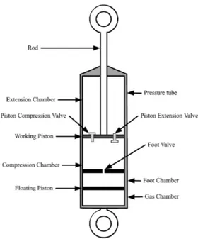
This vehicle suspension utilizes a single-tube telescopic damper, shown in Fig. 2.3.

Figure 2.3: Sectional view of a single-tube telescopic damper

The independent damper design variables are the valve diameter D0, the

working piston diameter Dp and the damper stroke Ds, that is the total

available axial displacement.

The damping coefficient is finally computed as

cs = D4 p 8CdC2D20 √ πkvρ1 2 (2.5)

Where Cd, C2, kv and ρ1 are coefficients of the damper calculated as in [1].

Finally, the vector of the plant design variables is xp =[d, D, p, Na, D0, Dp, Ds

]T

(33)

2.2. Sequential and Simultaneous Co-Design Optimizations 19

2.2.2 Sequential Optimization

As explained in the introductory chapter, the sequential approach consists in two successive optimizations: the first on the plant and the second on the control design variables.

Plant

Optimization x OptimizationControl

∗

p x∗c x∗

Figure 2.4: Sequential optimization approach scheme

Here the first is performed directly on the passive system described by Eq. (2.1), while the active component of the suspension is implemented only

for the second optimization.

The cost function to minimize showed in Eq. (2.7) is the same for both the ramp and the rough road profile simulations

J = ∫ tf

0

(r1(zus− z0)2+ r2z¨s2+ r3u2)dt (2.7)

where the first, second and third term of the integral evaluate respectively the handling of the vehicle, the comfort of the driver and the energy cost, while r1, r2 and r3 are weights.

The total cost function is a linear combination of the ramp and the rough road profile ones

J = 0.01Jramp+ Jrough (2.8)

The plant design variables are bounded by the constraints listed in [1]. Here, only the upper and lower bounds xp ≤ xp ≤ xp are reported:

x_p =[0.005, 0.05, 0.02, 3, 0.003, 0.03, 0.1]T xp =[0.02, 0.4, 0.5, 16, 0.012, 0.08, 0.3]

(34)

Plant Design Optimization

As mentioned before, the plant design optimization is performed on the passive system described by Eq. (2.1), hence it’s clear that the third term of the cost function in Eq. (2.7) related to the energy cost is null.

The optimization is performed using an active-set algorithm from the MATLAB optimization toolbox.

The resulting plant design is

Table 2.1: Passive suspension plant design results

d 0.0128 m D 0.0667 m p 0.0393 m Na 5.8000 D0 0.0046 m Dp 0.0300 m Ds 0.1700 m

From which the spring stiffness and the damping rate are obtained: ks = 3.86 × 104N/m cs = 2.30 × 103N/m/s (2.10)

Input Optimization

For this second optimization, the free variables are the forces applied and held on the suspension every 10 time instants.

As mentioned before, the simulated time is tf = 1s while the sampling rate

is fs = 1000Hz, resulting in Nt = 1000time instants. This implies a total

of Nu = 100 control actuations.

The final control design variables vector is then xc =[u1, u2, . . . , uNu, uNu+1, . . . , u2Nu

]T

(2.11) where the first Nu terms refer to the ramp simulation, while the last Nu

to the rough road simulation. This implies a total of 200 control design variables.

(35)

2.2. Sequential and Simultaneous Co-Design Optimizations 21 0 100 200 300 400 500 600 700 800 900 1000 Time [ms] -2000 -1500 -1000 -500 0 500 1000 1500 Force [ N]

Ramp Simulation Actuated Force

0 100 200 300 400 500 600 700 800 900 1000 Time [ms] -600 -400 -200 0 200 400 600 Force [ N]

Rough Road Simulation Actuated Force

Figure 2.5: Opimized actuated force for the ramp (left) and the rough road (right) simulations after a sequential optimization

The system in Eq. (2.1) is updated in order to consider the effect of the actuator on the state variables, as shown in Eq. (2.12).

˙ ξ = Aξ + B ˙z0+ Buu Bu = ⎡ ⎢ ⎢ ⎣ 0 − 1 mus 0 1 ms ⎤ ⎥ ⎥ ⎦ (2.12)

The only bound applied is the maximum absolute value of the applicable force, in this case:

|ui| ≤ 2000N 1 ≤ i ≤ 2Nu (2.13)

This optimization is implemented using an active-set algorithm, from the MATLAB optimization toolbox.

The resulting control design variables are shown in Fig. 2.5, while the final cost is shown in Table 2.2, where it is compared to the resulting cost of the passive suspension optimization.

Table 2.2: Passive and sequential optimization cost

JP as JSeq

(36)

2.2.3 Simultaneous Co-Design Optimization

The simultaneous optimization, as already mentioned in the introductory chapter, consists in a unique optimization of both the plant and control design variables, as in Fig. 2.6.

Plant and Control Optimization

x∗

Figure 2.6: Simultaneous optimization approach scheme

The unique vector of optimizing variables x is now the composition of plant xp and control xc design ones.

x =[d, D, p, Na, D0, Dp, Ds, u1, . . . , uNu, uNu+1, . . . , u2Nu

]T

(2.14) The set of linear differential equations describing the dynamic response of this system is directly the enlarged one in Eq. (2.12).

This optimization is performed using the active-set algorithm from the MATLAB optimization toolbox.

The resulting cost is in Table 2.3, where it’s shown that this approach generates a superior design (∼ 10% lower objective function value) with respect to the sequential one.

Table 2.3: Passive, sequential and simultaneous optimization cost

JP as JSeq JSim

3.8564 3.0938 2.7914

The optimized plant design variables are shown in Table 2.4 and compared to the sequential results, between their lower and upper bounds. It’s noteworthy how some of this variables have very different values from the two kinds of optimization.

(37)

2.3. Nested Co-Design Optimizations 23 0 100 200 300 400 500 600 700 800 900 1000 Time [ms] -2000 -1500 -1000 -500 0 500 1000 1500 Force [ N]

Ramp Simulation Actuated Force

0 100 200 300 400 500 600 700 800 900 1000 Time [ms] -800 -600 -400 -200 0 200 400 600 Force [ N]

Rough Road Simulation Actuated Force

Figure 2.7: Opimized actuated force for the ramp (left) and the rough road (right) simulations after a simultaneous optimization

Table 2.4: Comparison between sequential and simultaneous plant design vari-ables x_p xpseq xpsim xp d [m] 0.005 0.0128 0.0143 0.02 D [m] 0.05 0.0667 0.1288 0.4 p [m] 0.02 0.0393 0.05 0.5 Na 3 5.8 4.2587 16 D0 [m] 0.003 0.0046 0.0072 0.012 Dp [m] 0.03 0.03 0.0356 0.08 Ds [m] 0.1 0.17 0.17 0.3

2.3 Nested Co-Design Optimizations

As mentioned in the introductory chapter, the nested co-design optimization consists in an outer plant optimization problem, whose cost and constraints include the solution to an inner control optimization problem.

The plant design optimization is performed using a large-scale interior-point algorithm from the MATLAB optimization toolbox, while the internal loop is solved in two different ways.

The plant and control design variables are xp =[d, D, p, Na, D0, Dp, Ds

]T

xc=[u1, u2, . . . , uNu, uNu+1, . . . , u2Nu

]T (2.15)

(38)

24 Chapter 2. Co-Design of an Active Suspension System First a large-scale interior-point algorithm is used for the internal opti-mization too, returning the cost shown in Table 2.5.

Table 2.5: Passive, sequential, simultaneous and nested optimization cost

JP as JSeq JSim JN est

3.8564 3.0938 2.7914 2.9030

As expected, this co-design optimization method provides a design that is better with respect to the sequential one, but worse than the simultaneous one.

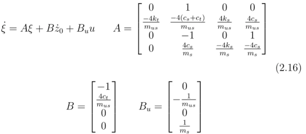
2.3.1 Quadratic Programming

Since the internal loop is performed each time with fixed plant design variables xp, the matrices A, B and Bu in Eq. (2.16) are well defined and

constant for each control design optimization.

˙ ξ = Aξ + B ˙z0 + Buu A = ⎡ ⎢ ⎢ ⎣ 0 1 0 0 −4kt mus −4(cs+ct) mus 4ks mus 4cs mus 0 −1 0 1 0 4cs ms −4ks ms −4cs ms ⎤ ⎥ ⎥ ⎦ (2.16) B = ⎡ ⎢ ⎢ ⎣ −1 4ct mus 0 0 ⎤ ⎥ ⎥ ⎦ Bu = ⎡ ⎢ ⎢ ⎣ 0 − 1 mus 0 1 ms ⎤ ⎥ ⎥ ⎦

This implies that the control design optimization can be solved as a quadratic programming problem.

This problems are solved by minimizing a cost function in the form J = 1

2x

T_{Hx + f}T_x _(2.17)

where x is the vector of variables to minimize while H and f are matrices. In this case x is the vector of control design variables xc, hence

(39)

2.3. Nested Co-Design Optimizations 25

xc=[u1, u2, . . . , uNu

]T

(2.18) In order to simplify the calculations, only the control variables for the ramp simulation are considered, since the rough road cost function derivation is identical.

Starting from the original cost function J =

∫ tf

0

(r1(ξ1)2+ r2( ˙ξ4)2+ r3u2)dt (2.19)

In order to obtain the equivalent H and f matrices for Eq. (2.17), one shall consider that

ξ1 = Adξ0+ Bdz00+ Budu1 (2.20)

where ξ1 is the vector of the values of the state variables at the first

time instant, ξ0 refers to the initial condition of the state variables, z00

is the initial condition of the road profile z0, and u1 is the first actuated

force, hence the first control design variable, while Ad, Bd and Bud are the

equivalent discrete-time matrices calculated with the trapezoidal method. Considering that the force is actuated every ten time instants, the vector containing the second values of the state variables is

ξ2 = Adξ1+ Bdz01+ Budu1 (2.21)

By substituting Eq. (2.20) in Eq. (2.21)

ξ2 = A2dξ0+ AdBdz00+ Bdz01+ (A1d+ A 0

d)Budu1 (2.22)

In this way the values of the state variables are calculated for every time instant of the simulation

ξ1 = F1ξ0+ G1Z01+ K1U1

ξ2 = F2ξ0+ G2Z02+ K2U2

...

ξNt = FNtξ0+ GNtZ0+ KNtU

(40)

26 Chapter 2. Co-Design of an Active Suspension System where Z0i is the vector containing the values of the road profile for any

time instant up to time i, Ui is the vector containing the actuated forces

up to time i and Fi = Aid Gi =[Adi−1Bd . . . A1dBd A0dBd ] Ki =[(Ai_d+ · · · + Ai−9_d )Bud . . . (A f d+ · · · + A 0 d)Bud ] (2.24)

where f is the remainder after i 10.

The derivative of the state variables is computed at any time instant as ˙

ξi = Aξi+ Bz0i+ Buui (2.25)

in which, substituting Eq. (2.23) ˙ ξi = dFiξ0+ dGiZ0i+ dKiUi (2.26) where dFi = AFi dGi =[AAi−1d Bd . . . AA1dBd AA0dBd+ B ] dKi =[A(Aid+ ... + A i−9 d )Bud . . . A(A f d+ · · · + A 0 d)Bud+ Bu ] (2.27)

with A, B and Bu the dynamic matrices of the system in Eq. (2.16).

The discrete time equivalent of the cost function in Eq. (2.19) is then J = Ts(r1(F[1]ξ0+ G[1]Z0+ K[1]U )T(F[1]ξ0+ G[1]Z0+ K[1]U )+

+ r2(dF[4]ξ0+ dG[4]Z0+ dK[4]U )T(dF[4]ξ0+ dG[4]Z0 + dK[4]U ) + r3UTU )

(2.28) with Ts the sampling time,

F[1] = C1F G[1] = C1G J[1] = C1J

dF[4] = C4dF dG[4] = C4dG dJ[4] = C4dJ

(41)

2.3. Nested Co-Design Optimizations 27 where C1 = [1 0 0 0] and C4 = [0 0 0 1] select respectively the

first and fourth state variables, and

F = ⎡ ⎢ ⎢ ⎢ ⎣ F1 F2 ... FNt ⎤ ⎥ ⎥ ⎥ ⎦ G = ⎡ ⎢ ⎢ ⎢ ⎣ G1 G2 ... GNt ⎤ ⎥ ⎥ ⎥ ⎦ K = ⎡ ⎢ ⎢ ⎢ ⎣ K1 K2 ... KNt ⎤ ⎥ ⎥ ⎥ ⎦ dF = ⎡ ⎢ ⎢ ⎢ ⎣ dF1 dF2 ... dFNt ⎤ ⎥ ⎥ ⎥ ⎦ dG = ⎡ ⎢ ⎢ ⎢ ⎣ dG1 dG2 ... dGNt ⎤ ⎥ ⎥ ⎥ ⎦ dK = ⎡ ⎢ ⎢ ⎢ ⎣ dK1 dK2 ... dKNt ⎤ ⎥ ⎥ ⎥ ⎦ (2.30)

In order to find the equivalent matrices H and f from Eq. (2.17), the cost function in Eq. (2.28) is reorganized and divided between the terms containing UT_U, U and the others.

J∗ =Ts(r1UTK[1]T K[1]U + r2UTdK[4]T dK[4]U + r3UTU +

+2r1(ξ0TF[1]TK[1]U + Z0TGT[1]K[1]U ) + 2r2(ξ0TdF[4]TdK[4]U + Z0TdGT[4]dK[4]U ))

(2.31) In Eq. (2.31) J∗ _{represent the effective cost function to minimize, since}

the terms neglected from Eq. (2.28) do not depend on the variables to optimize U.

Grouping the terms containing UT_U _{and the ones containing U one obtains}

J∗ =1 2U T (2Ts(r1K[1]TK[1]+ r2dK[4]T dK[4] + r310I))U + +2Ts(r1(ξ0TF T [1]K[1]+ Z0TG T [1]K[1]) + r2(ξ0TdF T [4]dK[4]+ Z0TdG T [4]dK[4])U (2.32) Where the 10 is needed since each control variable is applied for ten time instants, while I is the identity matrix.

(42)

28 Chapter 2. Co-Design of an Active Suspension System J∗ = 1 2U T_{HU + f}T_U H = 2Ts(r1K[1]T K[1]+ r2dK[4]T dK[4]+ r310I) f = (2Ts(r1(ξ0TF T [1]K[1]+ Z0TG T [1]K[1]) + r2(ξ0TdF T [4]dK[4]+ Z0TdG T [4]dK[4]))T (2.33) Constraints

The linear constraints depending on the control variables xc are solved as

part of the quadratic problem, as

Axc ≤ b (2.34)

Where A is a m × Nu matrix, xc is the Nu× 1control variables vector and

b a m × 1 vector such as, for every row of A, a single dis-equation in the form

A(i, :)xc≤ b(i) (2.35)

is solved.

Since at the first iteration of the outer loop the plant design variables are not optimal, it’s easy that the internal control design optimization cannot satisfy this constraints for any control design variables vector, resulting in a failed internal optimization.

To solve this issue soft constraints are applied, meaning that every con-straint is rewrote in the form

A(i, :)xc ≤ b(i) + α α ≥ 0 (2.36)

Eq. (2.36) is rewritten to contain all constraints, as in Eq. (2.34) ˜

A ˜xc ≤ ˜b (2.37)

(43)

2.3. Nested Co-Design Optimizations 29 ˜ A =[A −1 0 −1 ] ˜ xc= [xc α ] ˜ b = [b 0 ] (2.38) Where α is a parameter free to assume a value as big as necessary during the internal loop optimization in order to satisfy all the constraints in Eq. (2.37).

The last matrix modification to apply concerns the matrices H and f from the quadratic cost function in Eq. (2.17), since they fit the control variables vector xc dimensions.

˜ H =[H 0 0 γ ] ˜ f =[f 0 ] (2.39) where γ = 1000 is a fixed parameter with high value that multiplies α in the quadratic function cost. This expedient forces the solver to use the smallest α as possible, hence reducing as much as possible the maximum constraint violation.

Considering now the external plant optimization cost function J =

∫ tf

0

(r1(zus− z0)2+ r2z¨s2+ r3u2)dt (2.40)

a term concerning the maximum constraint violation of the internal loop is added, multiplied again by a fixed high value parameter. This mathematical expedient forces the external optimization to produce a plant design able to minimize the constraint violations in the internal loop.

The internal control design optimization, when fed with the optimal plant design, is able to solve the problem with α = 0, hence with all the original constraints satisfied.

Optimization

Applying a nested co-design optimization and solving the internal loop as a quadratic programming problem, the same result as the previous nested optimization is obtained.

This quadratic programming problem however can be seen as a model predictive control (MP C) with the prediction horizon covering all the simulated time.

(44)

30 Chapter 2. Co-Design of an Active Suspension System diminishing the size of the matrices F , G, K, Z0 and U.

Taking in example a prediction horizon of 50ms, matrix F and G contain data only for 50 time instants instead of 1000, while U is composed only by 5 control variables instead of 100. This means that, during the internal optimization, each control variable is optimized assuming to know only the next 50 time instants, and not the whole 1000.

Table 2.6: Nested co-design optimization with MPC for different values of the prediction horizon

Prediction Horizon [ms] 50 100 200

JM P C 3.4072 3.0731 2.9355

Results for nested co-design optimizations with different prediction horizons are displayed in Table 2.6. As expected, reducing the prediction horizon, the cost worsens.

It is notable however how with a nested co-design optimization with prediction horizon of just 100ms, that is one tenth of the total simulated time, a superior design is obtained with respect to a sequential one.

2.3.2 Conclusions On Co-Design methods

The results obtained with this experiment show how co-design is not only recommended, but becomes necessary when dealing with plant and control design optimization.

In addition, after a direct comparison between the main co-design tech-niques, the simultaneous one is demonstrated to perform best, therefore has been chosen to be applied on the winch-spring control system described in the next chapters.

(45)

Chapter 3 Co-Design of a Winch-Spring

Control System for a

Tethered-Drone with Base

Station on Ground

The need for tethered drones comes from the small autonomy of standard battery-equipped ones. Even the best ones can’t guarantee more than 30-35 minutes flights before a battery recharge is needed. This limit is difficult to overcome since bigger batteries would weigh more on a drone, requiring more power to fly.

Tethered drones solve this issue, having available through the tether all the power needed. The loss of range is the price to pay to avoid constant battery-needed returns, and for some kind of tasks, like surveillance, this loss doesn’t represent a concrete issue.

The system described in this chapter is the one shown in Fig. 3.1. A drone is linked with a tether to a winch fixed on a base station on the ground. The drone is free to fly anywhere above the base station within a range equal to the tether length.

(46)

32

Chapter 3. Co-Design of a Winch-Spring Control System for a Tethered-Drone with Base Station on Ground

1

2 3

4

Figure 3.1: Winch-Spring base station for the tethered drone. The winch (1) reels-in and out the tether (3). The spring (2) is compressed by the tether according to the drone (4) displacements.

The winch main objective is to reel-in and out the tether in order to follow the drone movements. A stretched cable could generate tugs, steering the drone away from its trajectory, while a tether too loose would weigh more than necessary on the drone, requiring more energy than needed.

To achieve this task, a spring is implemented on the base station, along with a position sensor on its extremity. When the tether is too stretched the spring is compressed, while a loose tether brings the spring back to its equilibrium position.

In this chapter first the drone model and control are shown, then the tether model adopted is explained and finally the winch control strategy involving the spring is described.

The overall block diagram of this system is shown in Fig. 3.2, where XD

are the drone coordinates, FT the tether force, Xs the spring compression,

T the torque applied on the winch and ϑ the winch angle.

Drone Tether Spring Winch Controller Base Station XD FT FT Xs T θ

(47)

3.1. Drone 33

3.1 Drone

The drone utilized in this system is a quadcopter (quadrotor helicopter), that consists intrinsically of a rigid body with four rotors propelled by brushless electric motors usually arranged at the corners of a rigid cross frame, as shown in Fig. 3.3.

Figure 3.3: Quadcopter and its reference axis

Choosing accordingly the rotational speed of each rotor, is possible to control the total trust and torque applied on the drone, both in absolute value and direction.

The model utilized for the drone dynamics is derived from [8],[9],[10], while the control strategy applied is the same as the one from [3].

3.1.1 Coordinate System

First an inertial right-handed reference G = X, Y, Z is introduced, centred on the base station, with the Z-axis pointing upwards. A local reference is also considered on the drone D = (x, y, z).

In order to translate from the inertial coordinates G to the local ones D, the following formula is used:

PD(t) = R(t)PG(t) (3.1)

where PD(t) and PG(t) are the drone coordinates respectively in the local

(48)

34

PD(t) = ⎡ ⎣ Px(t) Py(t) Pz(t) ⎤ ⎦ PG(t) = ⎡ ⎣ PX(t) PY(t) PZ(t) ⎤ ⎦ (3.2)

while R(t) is the rotation matrix defined as follows

R(t) = ⎡

⎣

cos(ψ)cos(ϑ) cos(ψ)sin(ϑ)sin(φ) − sin(ψ)cos(φ) cos(ψ)sin(ϑ)cos(φ) + sin(ψ)sin(φ) sin(ψ)cos(ϑ) sin(ψ)sin(ϑ)sin(φ) + cos(ψ)cos(φ) sin(ψ)sin(ϑ)cos(φ) − cos(ψ)sin(φ)

−sin(ϑ) cos(ϑ)sin(φ) cos(ϑ)cos(φ)

⎤

⎦

(3.3) Where ψ(t), ϑ(t) and φ(t) represent respectively the yaw, pitch and roll of the drone, hence the Euler angles providing its attitude with respect to the inertial system. The time dependence of this angles is omitted in Eq. (3.3) for the sake of space.

Through the rotation matrix, it’s also possible to translate from local to inertial coordinates, simply using its inverse, that is also its transpose R−1 = RT_.

Finally the time derivatives of the Euler angles are obtainable from the drone angular velocity with respect to its local axis (p, q, r) by means of

⎡ ⎣ ˙ φ ˙ ϑ ˙ ψ ⎤ ⎦= ⎡ ⎣ 1 sin(φ)tan(ϑ) cos(φ)tan(ϑ) 0 cos(φ) −sin(φ) 0 sin(φ)/cos(ϑ) cos(φ)/cos(ϑ) ⎤ ⎦ ⎡ ⎣ p q r ⎤ ⎦ (3.4)

3.1.2 Quadcopter Model

First the lift forces Li and drag torques Ti generated by the four rotors

are introduced:

Li(t) = bΩ2i i = 1, . . . , 4

Ti(t) = dΩ2i i = 1, . . . , 4

(3.5) where the index i refers to the rotors, Ωi is the rotational speed of the ith

rotor and b, d are respectively the rotors lift and drag coefficients.

Then the four lift forces and drag torques are linearly combined into four inputs u1...4(t) corresponding to the total lift over the z axis and to the

(49)

3.1. Drone 35 u1(t) = 4 ∑ i=1 Li(t) u2(t) = ar(L4− L2) u3(t) = ar(L3− L1) u4(t) = (T2+ T4) − (T1+ T3) (3.6)

where ar is the distance between each rotor and the drone centre of gravity.

Finally the equation of motion of the tethered drone:

¨ PG= 1 md ( RT ⎡ ⎣ 0 0 u1 ⎤ ⎦+ FtD − ⎡ ⎣ 0 0 g ⎤ ⎦ ) ˙ p = Iy − Iz Ix qr + u2 Ix − JP Ix qΩr ˙ q = Iz− Ix Iy pr + u3 Iy − JP Iy pΩr ˙r = Ix− Iy Iz pq +u4 Iz (3.7)

where g is the gravity acceleration, Ix, Iy and Iz are the drone rotational

moments of inertia on the three inertial axis, JP is the moment of inertia

of each motor on the drone, md is the drone mass and FtD is the tether

force acting on the drone, whose computation is shown in the next section of this chapter.

3.1.3 Control

For what concerns the drone controller, a hierarchical one is implemented, consisting in three nested loops as shown in Fig. 3.4.

Inertial position controller Local velocity controller Attitude and Altitude controller Drone

Pref PXref,PYref

PZref,ψref Pxref . Pyref . φref θref u1 ,u2 u3 ,u4 φ,θ,ψ,φ,θ,ψ,Pz,Pz . . . . Px,Py . . PX,PY

(50)

36

Chapter 3. Co-Design of a Winch-Spring Control System for a Tethered-Drone with Base Station on Ground To track reference attitude, hence roll, pitch and yaw, and altitude values, a static, multi-variable linear controller manipulates the rotor speeds. This controller is implemented according to the following linear model, derived from Eq. (3.4) and (3.7)

¨ PZ(t) = u1(t) md − g + dz(t) ¨ φ(t) = u2(t) Ix + dφ(t) ¨ ϑ(t) = u3(t) Iy + dϑ(t) ¨ ψ(t) = u4(t) Iz + dψ(t) (3.8)

where dz(t), dφ(t), dϑ(t)and dψ(t)are addictive terms accounting for errors,

and takes the following form:

⎡ ⎢ ⎢ ⎣ u1(t) u2(t) u3(t) u4(t) ⎤ ⎥ ⎥ ⎦ = K_dA ⎡ ⎢ ⎢ ⎢ ⎢ ⎢ ⎢ ⎢ ⎢ ⎢ ⎢ ⎣ PZref(t) − PZ(t) − ˙PZ(t) φref(t) − φ(t) − ˙φ(t) ϑref(t) − ϑ(t) − ˙ϑ(t) ψref(t) − ψ(t) − ˙ψ(t) ⎤ ⎥ ⎥ ⎥ ⎥ ⎥ ⎥ ⎥ ⎥ ⎥ ⎥ ⎦ + ⎡ ⎢ ⎢ ⎣ mdg 0 0 0 ⎤ ⎥ ⎥ ⎦ (3.9) where KA

d ∈ R4×8 is a static gain matrix computed via pole-placement.

It’s noteworthy how the gravity force is compensated with a feed-forward contribution.

The second controller, responsible in the middle control loop to compute the reference roll and pitch angles φref and ϑref, is implemented according

to the linearised model

¨

Px(t) = gϑref(t) + dx(t)

¨

Py(t) = −gφref(t) + dy(t)

(51)

3.1. Drone 37 where dx(t) and dy(t) accounts for tracking errors between φref, ϑref and

φ(t), ϑ(t).

The reference roll and pitch angles are then computed as: [ϑ_ref(t) φref(t) ] = K_dV [ _˙ Pxref(t) − ˙Px(t) −( ˙Pyref(t) − ˙Py(t)) ] (3.11) where KV

d is computed via pole-placement based on the model in Eq.

(3.10).

A third static linear controller computes the reference velocity vector ˙PGref

in order to track a desired position in the inertial coordinate G. The model on which it is based is:

˙

PX(t) = ˙PXref(t) + eX(t)

˙

PY(t) = ˙PYref(t) + eY(t)

(3.12)

where eX(t)and eY(t)are the tracking errors of the velocity components.

The outer controller takes the form: [ _˙ PXref(t) ˙ PYref(t) ] = K_dP [PXref(t) − PX(t) PYref(t) − PY(t) ] (3.13) where KP

d is again computed with pole-placement based on the model in

Eq. (3.12).

Finally, in order to be usable by the local velocity controller, the reference speed values are converted from the inertial to the local coordinate system as follows: [ _˙ Pxref(t) ˙ Pyref(t) ] =[ cos(ψ(t)) sin(ψ(t)) −sin(ψ(t)) cos(ψ(t)) ] [ _˙ PXref(t) ˙ PYref(t) ] (3.14) The values of the parameters listed in this section are in Table 3.1.

(52)

38

Table 3.1: Fixed drone parameters values

Name Symbol Value

x-axis rotational moment of inertia Ix 0.1032kg · m2

y-axis rotational moment of inertia Iy 0.1032kg · m2

z-axis rotational moment of inertia Iz 0.2472kg · m2

Drone mass md 10.9200kg

Rotor-centre of gravity distance ar 0.9m

Lift coefficient b 0.0017N · s2

Drag coefficient d 2.4 · 10−4N · s2

Motor inertia JP 3.4 · 10−5kg · m2

3.2 Tether

The model adopted to simulate the tether dynamics consists in splitting the unwrapped tether in a fixed number of equal segments.

The main goal of this model is to provide, at every time instant of the simulation, the values of the forces applied by the tether on the base station and the drone.

In [3] a simple approximation is applied, only the effective length of the tether with respect to the unrolled one is considered, hence the force on the ends of the tether results:

Ft(t) = max(0, kt(Ddrone− lt(t))) (3.15)

where Ddrone is the distance between the drone and the base station, kt is

the tether stiffness and lt is the unwrapped tether length. lt depends on

the winch rotation, as further explained in section 3.3. The maximum op-eration avoids the case of negative elastic force, since when the unwrapped tether length is greater then the distance between drone and base station the tether is loose, hence its elastic force is null.

This approximation doesn’t take in account the effect of the gravity force. In particular it could be split between the drone and the base station, and

(53)

3.2. Tether 39 not acting only on the first one.

That is why a more accurate model is implemented for the tether.

Base Station

ls

Figure 3.5: Tether model

Fig. 3.5 shows how the tether is divided in a fixed number Ns of segments,

with resulting length ls(t) = lt(t)/Ns, where lt(t) is the unwrapped tether

length.

The time dependency of the segment length ls(t) means that at any time

instant the number of segments Ns is constant, while the segment length

can vary according to the unwrapped tether one.

Every segment is modelled as a spring and damper system, as shown in Fig. 3.6 were the damping rate β accounts for the internal friction of the tether.

(54)

40

β

β kt

k_t

Figure 3.6: Segment model

The tether is hence split in Ns segments and Nn= Ns+ 1nodes, with first

and last nodes being the base station and the drone respectively.

Base Station X Z Y x y αplane

Figure 3.7: Base-Tether-Drone vertical plane

Considering that the tether, the base station and the drone lie on a vertical plane, as shown in Fig. 3.7, the coordinates of the base station and the

(55)

3.2. Tether 41 drone are translated from the inertial 3D reference to the new local 2D one, as follows: PG∗ =[√X2 G+ YG2 ZG ]T PD∗ =[√X2 D + Y 2 D ZD ]T (3.16)

where PG∗ and P_D∗ are the coordinates of the base station and the drone

with respect to the planar reference, XG, YG, ZG are the base station

coordinates in the inertial reference and XD, YD, ZD the drone inertial

coordinates.

In Eq. (3.16) is shown how the new plane is parallel to the tether, with vertical axis y equal to the vertical axis of the inertial reference Z. In particular, this plane is described by the angle between the new x − axis and the inertial X − axis, computed as

αplane = tan−1

( XD− XG

YD− YG

)

(3.17)

Each Nn node is studied by its position xi, yi and its speed ˙xi, ˙yi split in

the two axis component.

This leads to a total of 4Nn state variable, minus the base station and

drone ones, since their position and velocity are always known: the base station position is fixed, with zero velocity, while the drone dynamics are computed as in the previous section of this chapter.

The effective number of state variables is then 4(Nn− 2), where for each

node i they are defined as:

ξ_i = ⎡ ⎢ ⎢ ⎣ ξ1i ξ2i ξ3i ξ4i ⎤ ⎥ ⎥ ⎦ = ⎡ ⎢ ⎢ ⎣ xi ˙xi yi ˙ yi ⎤ ⎥ ⎥ ⎦ (3.18)

(56)

42

x y F_si F_si-1 Fxsi Fxsi-1 Fysi-1 Fysi Fg

Figure 3.8: Dynamic analysis of node i

The dynamical model on which this state variables are computed is derived from Fig. 3.8 where Fsi is the force transmitted to the node by the i

th

segment, Fx_si and Fy_si are its components with respect to the x − axis and

y − axis, while Fg is the weight force acting on the ith segment, defined as

Fg = msg (3.19)

with g the acceleration of gravity, ms = m_N_st the mass of the single segment

where mt = ρtlt is the total mass of the the unwrapped tether, ρt its linear

density and lt the unwrapped tether length.

The force Fsi transmitted by a segment i to a node is the sum of the elastic

and viscous forces, hence

Fsi = Fki+ Fβi

Fki = max(0, kt(lsi − ls))

Fβi = βvsi

(3.20)

Here, kt is the tether segment stiffness, calculated as

kt=

Fmaxt

ltεt

(57)

3.2. Tether 43 with Fmaxt and εt the breaking load and elongation.

lsi is the effective length of segment i, which is different from its nominal

value ls only when the tether is stretched, and computed according to the

positions of the two nodes on its ends:

lsi = √ l2_x si + l 2 y_si lx_si = xi+1− xi ly_si = yi+1− yi (3.22)

where lx_si and ly_si are the segment length projection on the two coordinates,

while xi and yi are the coordinates on the two axis of the ith node.

Similarly, the ith_{segment velocity v}

si in Eq. (3.20) is computed, considering

the velocity of the two nodes on its ends:

vsi = √ v2 x_si + v2y_si vx_si = ˙xi+1− ˙xi vy_si = ˙yi+1− ˙yi (3.23)

with ˙xi and ˙yi the speed of the ith node on the two coordinates.

Then the elastic Fki and viscous force Fβi of the i

th segment are split into

their components on the two coordinates as:

Fk_xsi = Fk_sicos(αi)

Fk_ysi = Fk_sisin(αi)

Fβ_xsi = Fβ_sicos(αi)

Fβ_ysi = Fβ_sisin(αi)

(3.24)

where αi is the direction of the ith segment, computed as

αi = tan−1 (_l x_si ly_si ) (3.25)

(58)

44

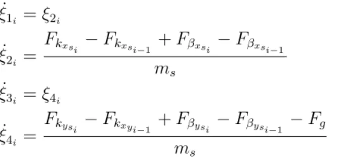
Chapter 3. Co-Design of a Winch-Spring Control System for a Tethered-Drone with Base Station on Ground Finally the dynamic model of Fig. 3.8 is derived, according to Eq. (3.18), by the Newton method, as

˙

ξ1i = ξ2i

˙ ξ2i =

Fk_xsi − Fk_xsi−1 + Fβ_xsi − Fβ_xsi−1

ms

˙

ξ3i = ξ4i

˙ ξ4i =

Fk_ysi − Fk_xyi−1 + Fβ_ysi − Fβ_ysi−1 − Fg

ms

(3.26)

where the index i accounts for the nodes.

The last task is to compute the forces acting on the two end nodes, hence the ground and the drone.

Their values, at each simulation time instant, split in their planar coordi-nates, are FtD = [ Fk_xsNn + Fβ_xsNn Fk_ysNn + Fβ_ysNn ] FtG = [_−F k_xs1 − Fβ_xs1 −Fk_ys1 − Fβ_ys1 ] (3.27)

Another advantage of this model lies in knowing the position of all the Nn

nodes, hence having clear information on how the cable is positioned at every time instant.

To translate the position of the nodes from planar to inertial 3D coordinates the following formula is used:

Xni = xicos(αplane)

Yni = xisin(αplane)

Zni = yi

(3.28)

where αplane is the angle the plane makes with the inertial X − axis,

computed by Eq. (3.17).

(59)

3.3. Base Station 45

Table 3.2: Fixed tether parameters values

Name Symbol Value

Number of segments Ns 51

Internal friction β 5N/m · s

Tether linear density ρt 0.03kg/m

Breaking load Fmaxt 5000N

Breaking elongation εt 0.03

3.3 Base Station

The base station utilized in this system is placed on the ground, and consists in a winch, responsible of the unrolling and withdrawing of the tether, and a spring necessary to control the aforesaid winch.

The innovative feature of this base station is the total decoupling between the drone and the base station itself, the former in fact is seen as a distur-bance, since no informations regarding its position or future movements are sent to the ground control system.

The control strategy that commands the winch is implemented by means of a spring, compressed when the tether is too tense, and in equilibrium position when it’s too loose.

The position sensor installed on the pulley on the movable end of the spring tells the system when to eel-in or out the tether.

Since it can only be compressed by the tether force, the possible dis-placement of the spring goes from the equilibrium position xs= 0 to the

(60)

46

Figure 3.9: Spring zones

Fig. 3.9 also shows how, for control purpose, the spring is divided in three fictitious zones.

The first, between xs= 0 and xs = xI, is the zone around the equilibrium

position, meaning that the tether is loose, hence commanding the winch to reel it in.

The second zone, between xI and xII, is where ideally the spring mass

should stay, meaning the tether is neither too stretched nor loose.

The last one, going from xIIto xsmax, is where the spring is most compressed.

This zone is reached only when the tether is too stretched, causing a strong force acting both on the base and drone end resulting in tugs and consequently not optimal performance of the drone. When the movable pulley is in this last zone, the winch should reel-out the tether.

This control strategy is further explained at the end of this section, after a small description of the model adopted for the base station.

3.3.1 Dynamic Model

The dynamic model for the base station is derived from the scheme in Fig. 3.10.

+

Ft Ft xs=0 T Jθ.. βθ.

Co-design optimization of a tethered multi drone system

Scuola di Ingegneria Industriale e dell’Informazione

Master of Science in Automation and Control

Engineering

Co-Design Optimization of a

Tethered Multi Drone System

Supervisor:

Prof. Lorenzo Mario FAGIANO

M.Sc. Thesis by:

Giovanni CLARIZIA

Matr. 875686

Contents

List of Figures

List of Tables

Abstract

Sommario

Chapter 1

Introduction

1.1

Motivation and Goals

1.2

Co-Design Techniques

1.3

Original Contributions of this Thesis

1.4

Thesis Outline

Chapter 2

Co-Design of an Active

Suspension System

2.1

Active Suspension Model

2.2

Sequential and Simultaneous Co-Design

Optimizations

2.2.1

Plant Design Variables

2.2.2

Sequential Optimization

2.2.3

Simultaneous Co-Design Optimization

2.3

Nested Co-Design Optimizations

2.3.1

Quadratic Programming

2.3.2

Conclusions On Co-Design methods

Chapter 3

Co-Design of a Winch-Spring

Control System for a

Tethered-Drone with Base

Station on Ground

3.1

Drone

3.1.1

Coordinate System

3.1.2

Quadcopter Model

3.1.3

Control

3.2

Tether

3.3

Base Station

3.3.1

Dynamic Model

+