Master of Science in Building Engineering
Academic year 2016/2017
An energy efficiency driven
algorithm for filtering and
sizing HVAC system layouts
for building retrofit
Supervisor: Prof. Rossano Scoccia
Master dissertation of Vincenzo Francesco Cirillo, 859090Il lavoro di tesi presentato in queste pagine non sarebbe stato possibile senza la partecipazione del mio relatore, il professor Rossano Scoccia, al quale va il mio più sentito ringraziamento per la continua spinta ad approfondire, per la competenza e per la disponibilità con le quali mi ha guidato in questi mesi. También quiero agradecer a Tecnalia, partner del proyecto Heat4Cool, por el apoyo durante los tres meses con ellos para llevar a cabo parte de esta investigación. En particular, agradezco a mis colegas y maestros Perú Elguezabal y Beñat Arregi, por la ayuda y la maravillosa hospitalidad.
Con questa tesi di laurea concludo idealmente il mio percorso di studi. Desidero quindi ringraziare anche tutti coloro che mi hanno accompagnato in questo lungo cammino.
Ringrazio il Politecnico di Milano, il Liceo Parini e l’Istituto Gonzaga per le opportunità che mi hanno concesso. Ringrazio tutti i docenti che in questi anni mi hanno cresciuto come studente e come persona. Ringrazio compagne e compagni di studio con cui ho condiviso questi momenti; in particolare, un ringraziamento va ad Ayu, Dario, Fabio e Giangio, non compagni bensì fratelli.
Ringrazio gli amici, anche quelli non juventini, persino quelli del FantaGreco. Ringrazio Mario per i suoi insegnamenti.
Ringrazio tutta la mia famiglia, zie, zii, cugini e i miei figliocci, Ludovica e Cristian. Ringrazio Laura e Luciano, che famiglia lo sono diventati.
Ringrazio Elisa di essere al mio fianco.
Ringrazio mia sorella Elena e mio fratello Daniele, di cui sono orgoglioso. Sono certo che anche loro arriveranno presto e brillantemente a questo traguardo.
Ringrazio immensamente i miei genitori. Chi li conosce sa quanto questo traguardo sia soprattutto merito loro.
Desidero infine dedicare questa tesi di laurea a mia nonna Teresa, che con straordinaria lungimiranza, in un ambiente tutt’altro che colto e benestante, capì l’importanza dell’istruzione, spendendosi ardentemente per assicurare alla sua famiglia ciò che lei non aveva potuto avere.
As reported in many sources, buildings consume over 40% of end-use energy worldwide, the quasi-totality destined for Heating, Ventilation and Air-Conditioning (HVAC) systems. Several studies dealt with the topic, developing new methods for the optimization with statistics, cost-optimal building design or through Multi-Criteria Decision Making. Inspired by the objectives of the European project Heat4Cool, I wanted to create a general algorithm for the pre-design of HVAC rehabilitation, i.e. a program for filtering all the possible solutions, size them and evaluate their performance. My work starts with the analysis of the building models which can be adopted for the purpose, looking at qualities and criticalities of the hourly static energy balance compared with TRNSYS dynamic simulation. Once defined this theoretical base, it is written with MATLAB a program that individuates some simple rules guided by standards and technical literature, in an ample engineering spectre, from mechanical to hydraulic and energy aspects. The filter and sizing are governed by the external inputs coming from an auxiliary front-end program, following a precise path in function of the interconnection of HVAC equipment. The rendering of the results is entrusted to a program which translates the HVAC layout into an energy rating index, the Primary Energy (PE) demand. It contains and applies the PE factors for the conversion of the annual energy need of the building system configurations, computed with reference to the machineries performance maps. I tested the program on a reference framework, placed in three different European climates, varying the envelope performance. The results confirm the expected energy savings earned with advanced HPs, solar plants and PCM: they are shown the PE demand profiles of HVAC solutions, the possibility or impossibility of the achievement of NZEB status and the relative importance of each component of the retrofit. Results demonstrate that the algorithm reads with precision the variations of boundary constrains, giving a comparative tool for the optimization of dynamic models or a replicable module for multi-variable analysis.
Sintesi
Come riportato in molte fonti, gli edifici consumano oltre il 40% dell'energia prodotta, la quasi totalità della quale destinata ai sistemi HVAC. Diversi studi hanno sviluppato metodi per l'ottimizzazione impiantistica, con metodi statistici, modelli economici o attraverso processi decisionali multi-criterio. Prendendo spunto dagli obiettivi del progetto europeo “Heat4Cool”, ho voluto creare un algoritmo di pre-progettazione del riammodernamento dei sistemi HVAC, ossia un programma in grado di filtrare le soluzioni significative, dimensionarle e valutarne le prestazioni. Il mio lavoro inizia con l'analisi dei modelli dell’edificio adatti allo scopo, studiando qualità e criticità del bilancio energetico statico orario rispetto alla simulazione dinamica di TRNSYS. Una volta definita questa base teorica, con MATLAB è stato scritto un programma che individua semplici relazioni, rielaborate da normative e letteratura tecnica, in un ampio spettro ingegneristico, dalla meccanica all’idraulica all’energetica. Filtraggio e dimensionamento sono guidati dagli input esterni di un programma front-end, seguendo un percorso preciso in funzione dell'interconnessione delle apparecchiature. Il rendering dei risultati è affidato a un programma che traduce le soluzioni HVAC in un indice di valutazione, ossia la domanda di energia primaria (PE). Il programma contiene e applica i fattori di PE per la conversione del fabbisogno energetico delle configurazioni impiantistiche, calcolato in riferimento alle efficienze dei macchinari. Ho testato il programma su un edificio di riferimento, collocato in tre diversi climi europei, variandone le prestazioni dell'involucro. I risultati confermano i risparmi energetici previsti da PdC d’avanguardia, impianti solari e PCM: si mostrano i profili del fabbisogno energetico delle soluzioni HVAC, la possibilità o meno dell’ottenimento di NZEB e l'influenza di ciascun componente nella riqualificazione. I risultati dimostrano che l'algoritmo legge con precisione le variazioni delle condizioni al contorno, fornendo uno strumento ausiliario per l'ottimizzazione di modelli dinamici ovvero un modulo replicabile per l'analisi multi-variabile.
Nomenclature ... 12
1 Introduction ... 14
1.1 Summary of the project Heat4Cool ... 14
1.2 Description of Work Package 2 ... 14
1.3 Connection between the project and the thesis work ... 16
2 Analysis of the building model adopted in the algorithm ... 18
2.1 The building energy model ... 18
Heat losses ... 18
Heat gains ... 19
2.2 Building dynamic simulation ... 20
2.3 Description of the reference building ... 22
2.4 Dynamic simulation of the reference building with TRNSYS models ... 25
2.5 Results and comments ... 27
3 The HVAC technologies contemplated by the algorithm ... 32
3.1 The HVAC system types ... 32
3.2 The emission subsystem... 33
3.3 The generation subsystem ... 34
Heat generators ... 34
Heat generation source ... 36
Renewable energy systems ... 36
3.4 Thermal energy storage ... 37
4 The filtering algorithm ... 38
4.1 Description of the procedure ... 38
4.2 The climate data ... 41
4.3 Acquisition of the inputs ... 44
4.4 The building energy demand ... 48
Energy demand for space heating and cooling ... 48
Domestic Hot Water demand estimation ... 50
4.5 The comparison with energy demand from TRNSYS models ... 51
4.6 The filtering algorithm with MATLAB ... 53
5 The sizing algorithm and the estimation of the energy demand... 62
5.1 Procedure for the sizing ... 62
Electric generators ... 64
Electric Heat-Pump/Chiller sizing... 65
Boiler sizing ... 65
5.2 The sizing algorithm with MATLAB ... 65
5.3 Estimation of the Primary Energy demand ... 72
Renewable energy systems and thermal storage ... 72
Heating and cooling generators ... 73
5.4 The estimation of the Primary Energy demand with MATLAB ... 75
6 Results and comments ... 84
6.1 Description of the program ... 84
6.2 SFH 100: comments ... 100
6.3 SFH 45: comments ... 106
6.4 SFH 15: comments ... 108
Conclusion ... 111
Bibliography ... 113 Annex I: Computation of the thermal characteristics of the reference framework for system simulations “Single Family House – SFH”
Annex II: TRNSYS deck file for the case “SFH 45” in Strasbourg
Annex III: Results of the comparative analysis between “Lumped capacitance building” and “Multi-Zone Building” on TRNSYS
Annex IV: MATLAB program ‘ReadEPW.m’ Annex V: MATLAB function ‘tilted_radtion.m’ Annex VI: MATLAB program ‘Inputs.m’
Annex VII: U-values for the countries in Heat4Cool project Annex VIII: MATLAB program ‘Energy_demand.m’ Annex IX: Results for Single Family House SFH 15 Annex X: Results for Single Family House SFH 45
Figure 1.1 - RetroSim layout with definition of the different phases of the simulation ... 16
Figure 2.1 - Global scheme of the building energy balance ... 18
Figure 2.2 - Typical profiles of internal and external temperature in winter ... 20
Figure 2.3 - Typical profiles of internal and external temperature in summer ... 21
Figure 2.4- Building general view ... 22
Figure 2.5 – TRNSYS network used for SFH 45 case in Strasbourg ... 25
Figure 2.6 - TRNBUILD configuration used for SFH 45 case in Strasbourg ... 26
Figure 2.7 - Maximum temperature difference between Type 88 and Type 56 in free floating conditions ... 27
Figure 2.8- Monthly average of the internal temperature for SFH15 in Strasbourg... 29
Figure 2.9- Monthly average of the internal temperature for SFH15 in Athens ... 29
Figure 2.10- Monthly average of the internal temperature for SFH15 in Helsinki ... 29
Figure 2.11 - Comparison of the annual heating demand ... 30
Figure 2.12 - Comparison of the annual cooling demand ... 30
Figure 3.1 - Ideal temperature/height curve of the thermal comfort ... 33
Figure 3.2 - Boiler efficiency in function of the load factor ... 35
Figure 3.3 - Scheme of the heat-pump cycle ... 35
Figure 3.4 - Solar power available in function of the tank type ... 37
Figure 3.5 - Dimension of PCM tank module ... 37
Figure 4.1 - Summary scheme of the heating system retrofit ... 39
Figure 4.2 - Summary scheme of the cooling system retrofit ... 40
Figure 4.3 - Schematic of the distribution of diffuse radiation over the sky dome ... 42
Figure 4.4 - Photo of a pyranometer ... 42
Figure 4.5 - Standard values for window properties ... 45
Figure 4.6 - Occupation and air change for class of building ... 48
Figure 4.7 - Internal gains for class of building ... 49
Figure 4.8 - Water demand per day for class of building ... 50
Figure 4.9 - Comparison of the annual heating demand ... 51
Figure 4.10 - Comparison of the annual heating demand ... 51
Figure 5.1 - Standard values of the peak power coefficient of a photovoltaic module ... 63
Figure 5.2 - Boiler efficiency in function of the load factor ... 73
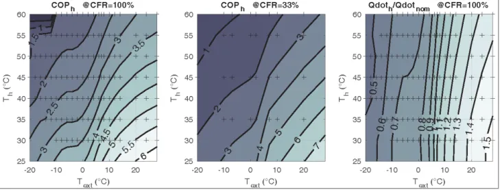
Figure 5.3 - COP of the heat pump in heating mode in function of the external temperature ... 74
Figure 5.4 - GUE of the heat pump in function of the external temperature ... 74
Figure 6.1 - Annual Primary Energy demand of the retrofit solutions for SFH 100 in Strasbourg ... 100
Figure 6.2 - Annual Primary Energy demand of the retrofit solutions for SFH 100 in Athens ... 100
Figure 6.3 - Annual Primary Energy demand of the retrofit solutions for SFH 100 in Helsinki ... 101
Figure 6.4 - PE demand comparison between the best retrofit solution and the existing HVAC system for SFH 100 in Strasbourg ... 102
Figure 6.5 - PE demand comparison between the best retrofit solution and the existing HVAC system for SFH 100 in Helsinki ... 102
Figure 6.6 - PE demand comparison between the best retrofit solution and the existing HVAC system for SFH 100 in Athens ... 104
Figure 6.7 - Annual Primary Energy demand of the retrofit solutions for SFH 45 in Strasbourg ... 106
Figure 6.8 - Annual Primary Energy demand of the retrofit solutions for SFH 45 in Athens ... 106
Figure 6.12 - Annual Primary Energy demand of the retrofit solutions for SFH 15 in Helsinki ... 109 Figure III.1 - Monthly average external temperature in the reference climates
Figure III.2 - Monthly average temperature difference between Type 88 and Type 56 in Strasbourg in free floating conditions
Figure III.3 - Monthly average temperature difference between Type 88 and Type 56 in Athens in free floating conditions
Figure III.4 - Monthly average temperature difference between Type 88 and Type 56 in Helsinki in free floating conditions
Figure III.5 - Monthly maximum temperature difference between Type 88 and Type 56 in Strasbourg in free floating conditions
Figure III.6- Monthly maximum temperature difference between Type 88 and Type 56 in Athens in free floating conditions
Figure III.7- Monthly maximum temperature difference between Type 88 and Type 56 in Hlesinki in free floating conditions
Figure III.8 - Monthly average of the internal temperature for SFH15 in Strasbourg Figure III.9 - Monthly average of the internal temperature for SFH15 in Athens Figure III.10 - Monthly average of the internal temperature for SFH15 in Helsinki
Table 2.A - Measures of building external surfaces ... 22
Table 2.B - The three different prototypes of building ... 22
Table 2.C - Constructive characteristics of the building ... 23
Table 2.D – Orientation and measure of the windows of the building ... 23
Table 2.E - Thermal and optical characteristic of the windows ... 23
Table 2.F - Resume of the global building parameters ... 24
Table 2.G - Profiles of the internal gains ... 24
Table 2.H - Average monthly difference between Type 88 and Type 56 output temperature in free floating conditions ... 27
Table 2.I - Temperature profiles in SFH 15 Athens... 28
Table 2.J - Comparison of the total energy demand ... 31
Table 4.A - Peak of the heating power demand along the year ... 52
Table 4.B - Peak of the cooling power demand along the year ... 52
Table 5.A - Standard values of the Primary Energy factor ... 72
Table 6.A - Main values of the total amount of Primary Energy demand for SFH 100 in Strasbourg ... 100
Table 6.B - Main values of the total amount of Primary Energy demand for SFH 100 in Athens ... 100
Table 6.C - Main values of the total amount of Primary Energy demand for SFH 100 in Helsinki ... 101
Table 6.D - Components of the best retrofit solution for SFH 100 in Strasbourg ... 103
Table 6.E – Focus on the Primary Energy savings for SFH 100 in Strasbourg ... 103
Table 6.F - Components of the best retrofit solution for SFH 100 in Helsinki ... 103
Table 6.G - Focus on the Primary Energy savings for SFH 100 in Strasbourg ... 103
Table 6.H - Components of the best retrofit solution for SFH 100 in Athens ... 105
Table 6.I - Focus on the Primary Energy savings for SFH 100 in Athens ... 105
Table 6.J - Main values of the total amount of Primary Enegry demand for SFH 45 in Strasbourg ... 106
Table 6.K - Main values of the total amount of Primary Energy demand for SFH 45 in Athens ... 106
Table 6.L - Main values of the total amount of Primary Energy demand for SFH 45 in Helsinki ... 107
Table 6.M - Main values of the total amount of Primary Energy demand for SFH 15 in Strasbourg .... 108
Table 6.N - Main values of the total amount of Primary Energy demand for SFH 15 in Athens ... 108
Table 6.O - Main values of the total amount of Primary Energy demand for SFH 15 in Helsinki ... 109 Table III.A - Monthly values of external temperaturs in the reference climates
Table III.B - Output temperatures in Strasbourg Table III.C - Output temperatures in Athens Table III.D - Output temperatures in Helsinki
Table III.E - Output energy demand for space heating and cooling in Strasbourg Table III.F - Output energy demand for space heating and cooling in Athens Table III.G - Output energy demand for space heating and cooling in Helsinki Table III.H- Comparison of the energy demand for space heating
Table III.I- Comparison of the energy demand for space cooling Table III.J- Comparison of the total energy demand
12
A Area [m2]
α Global gain factor [W/m2]
β Slope of the tilted surface [°]
C Thermal capacity [J/K]
COP Coefficient Of Performance of the Heat-Pump/Chiller [-]
cp,a Isobaric specific heat of air, in standard conditions is equal to 1.0005 [kJ/(kg∙°C)] cp,v Isobaric specific heat of water vapour, in standard conditions is equal to 1.95 [kJ/(kg∙°C)] cp,w Isobaric specific heat of liquid water, in standard conditions is equal to 4.186 [kJ/(kg∙°C)]
γ Azimuth angle [°]
dp Duration of the peak demand [h]
δ Solar declination angle [°]
E Thermal energy [kWh]
g Solar factor of the window [-]
GUE Gas Utilization Efficiency of the Heat-Pump/Chiller with natural gas support [-]
h Superficial heat transfer coefficient through convection [W/(m2∙K)]
ha Specific enthalpy of moist air [kJ/(kg∙K)]
HT Heat transfer coefficient for transmission through the envelope [W/K] HV Heat transfer coefficient for ventilation [W/K]
η Efficiency of the boiler [-]
θ Zenith angle [°]
IS Solar radiation [kW/m2]
Kpk Peak power coefficient of the photovoltaic module [kW/m2]
λ Thermal conductivity [W/(m∙K)]
λLV Latent heat of vaporization of water, in standard conditions is equal to 2501 [kJ/kg]
ṁa Air mass flow [kg/s]
np Occupancy rate [pers./m2]
p Pressure [Pa]
PE Primary Energy [kWh]
PEf Primary Energy factor [-]
13
Q̇ Thermal power [kW]
Rb Beam radiation ratio with respect to the total horizontal radiation [-]
ρ Density [kg/m3]
ρa Air density, in standard conditions is equal to 1.225 [kg/m3]
ρg Albedo coefficient [-]
ρw Water density, in standard conditions is equal to 1000 [kg/m3]
s Thickness [m]
t Time [s]
T Temperature [°C]
U Thermal transmittance [W/(m2∙K)]
vDHW Domestic hot water peak demand [l/h]
V Volume [m3]
φ Latitude [°]
X Absolute humidity of air [gw/kga]
14
1 Introduction
The inspiration of this thesis comes from Work Package 2 in Heat4Cool project. It deals with the design of the web-tool for retrofit named “RetroSim”, developed by a design team constituted by four partners who interact on its different aspects.
Chapter 1 briefly describes the whole project and the package, with a view to its primary objectives and the driving philosophy.
1.1 Summary of the project Heat4Cool
Heat4Cool proposes an innovative, efficient and cost-effective solution to optimize the integration of a set of rehabilitation systems in order to meet the net-zero energy standards. The project develops, integrates and demonstrates an easy to install and highly energy efficient solution for building retrofitting that begins from the Heat4Cool advanced decision-making tool (which addresses the building and district characteristics) and leads to the optimal solution combining:
- gas and solar thermally driven adsorption heat pumps, which permits the full integration with existing natural gas boilers to ensure efficient use of current equipment;
- solar PV assisted DC powered heat pump connected to an advanced modular PCM heat and cold storage system;
- energy recovery from sewage water with high performance heat exchangers.
“The project will implement four benchmark retrofitting projects in four different European climates to achieve a reduction of at least 20% in energy consumption in a technically, socially, and financially feasible manner and demonstrate a return on investment of 8 years. The Heat4Cool consortium will ensure the maximum replication potential of the Heat4Cool solution by a continuous monitoring of technical and economic barriers during the development and validation phases in order to present the building owners and investors with clear energy and economic evidence of the value of implementing Heat4Cool solution.”1
1.2 Description of Work Package 2
The objective is to develop a reliable design tool that will allow the simulation of the combination of different retrofitting measures (including HVAC, RES and BEMS measures) assessing the energy savings and the cost-effectiveness of the solutions and thus supporting the retrofitting decision making.
- Provide a mapping of existing buildings and districts energy performance
- Identification of needs and constraints for the selection of most suitable retrofitting measures. - Creation of a retrofitting tool kit Dataset with technological solutions and legislative requirements - Definition of the specifications of the design tool
- Definition of the algorithms that will allow assessing the most cost-effective retrofitting measures combination
- Implementation of the tool “RetroSim”
1 European commission, Directorate-general for research & innovation, #723935 - Heat4Cool: Smart building retrofitting
15 The specific description of the work is divided into five tasks.
Task 2.1.
Mapping of European building stock (identifying needs and constraints). Task 2.2.
Creation of the Heat4Cool Retrofitting tool kit Dataset It deals with two kinds of data:
- technology data: retrofitting measures will be collected, focusing on HVAC, RES integration, BEMS, and their interconnection. The technologies will be described with all the required information needed for the optimisation algorithms. Moreover, special requirements of each of them and of the interconnection between them will be included. The cost of each technology will be included for the cost-effectiveness analysis.
- Regulatory data: most relevant regulation will be identified in order to ensure the applicability of the proposed retrofitting solutions.
The toolkit data set will be a repository of technological solutions that will be open to updates. Task 2.3.
User requirements, technical specification and architecture design
The core functionalities will be defined, indicatively including functionalities such as i) analysis of building/district characteristics,
ii) modelling of available retrofitting solutions including control systems iii) energy efficiency estimation
iv) retrofitting cost estimation
v) validation of suggestion based on applicable regulation vi) data management
vii) user interface front-end. Task 2.4.
Creation of the optimisation algorithm for the solution set
The task leader along with the involved partners will build an optimisation model to provide a retrofitting solution set determined on the inputs from building characteristics (Task 2.1), technology options (Task 2.2) and user requirements (Task 2.3).
The optimization technique is constraint-based and will provide solutions with respect to Energy consumption, Carbon emissions, Payback period (PBP) and Life-Cycle Cost Analysis (LCCA). The constraints and objectives are based on the user information entered via the web portal and the constraints that have been collected about National Building Codes, HVAC functional and non-functional requirements and user specifications. The optimization tool will ensure the best retrofitting choice in terms of typology, resources and size for each demo case, orienting to the end user as decision support platform in HVAC retrofitting design.
Task 2.5.
16
1.3 Connection between the project and the thesis work
Heat4Cool is a pluriannual project which aims to diffuse some retrofit solutions for European buildings. Part of its work is the development of the webtool RetroSim from which I took inspiration for my thesis. The design layout2 of the tool is represented in Figure 1.1.
2 Heat4Cool - Smart building retrofitting complemented by solar assisted heat pumps integrated within a self-correcting
intelligent building energy management system.
Task 2.5 - User Interface design and tool integrated development. Figure 1.1 - RetroSim layout with definition of the different phases of the simulation
17 The primary objective of my thesis is the achievement of a set of simple rules that build an algorithm for the filtering of all the possible retrofit solutions that nowadays can be encountered on the market. This derives from the necessity, in RetroSim, of an instrument, called “Optimizer”, which can select just few interesting HVAC layouts for its dynamic simulation.
The first part of the work is the design of some substitutive program which can perform the computation of the energy balance of the building and the dialogue with the user, for the acquisition of the fundamental inputs for the optimization.
My work started with the analysis of the different models which can be adopted for the study of the building, looking at their qualities and criticalities, analysing especially the reliability of the assumptions made for the obtainment of a tool which can be in the same time efficacious and not burdensome. I compared the results coming from annual static simulations and the outputs of a reference dynamic simulation software (TRNSYS).
Once known the different aspect of the adopted model, I wrote on MATLAB an auxiliary front-end and only at this point I could write the actual rules and the logic of the filtering tool. The program is based on several rules I could find in the technical literature, guided by the experience I acquired in these years on building systems and its machineries. I looked at the topic in an ample spectre, from mechanical to hydraulic and above all the energy engineering.
I decided to differentiate my approach from the one chosen in Heat4Cool project for the tool RetroSim, because it was focused on some reference HVAC system layouts based on the most strong and modern technologies involved in the project (DC heat-pump, adsorption heat-pump, PCM storage), while, on the other hand, I preferred to leave this constrain, in order to attain a more general algorithm which can be replicated for different purposes out of the project Heat4Cool. It is important to underline, anyway, that the results of my thesis also confirmed the validity of the choice made by Heat4Cool team.
The sizing program checks the performance of the equipment against the building energy demand, together with some assessments also on the commercial aspects of the size of the generators. Once again, I referred to the available literature and the standards that rule the subject.
For the obtainment of a visualization of the outputs, I wrote a program which translates the set of HVAC system layouts into a rating index. I decided to do so with the Primary Energy demand, that is the most used parameter for the evaluation of the energy performance of buildings. The program explores the necessary information in some selected performance maps which let me render the hourly HVAC need of the building with the Primary Energy demand of the building system.
This last program rates the retrofit solutions from the energy point of view, but this is not the only topic that has to be evaluated in the design. RetroSim project adopts a multiple rating of the most interesting solutions, after its simulation engine analyses the building energy balance in its differential form that permits to study also the internal temperature profiles, hence the comfort of the users and the control of the emission subsystem. My program “PE_demand” could be seen as the module for RetroSim multi-criteria evaluation, with the AHP (Analytical Hierarchy Process) that translates the preferences of the users and can satisfy them in a wider way.
The thesis finishes with the run of the program on the reference framework adopted, obtaining the expected results and looking at the fact that algorithm can read with precision the different behaviour of the building in the different European climates. In the end the program resulting is a pre-desing tool for HVAC retrofit, whose greatest potential comes out together with a dynamic simulation of the outputs and multi-criteria decision analysis.
18
2 Analysis of the building model adopted in the algorithm
My program bases its calculation on the building energy model commonly used in classical thermodynamics, whose the cardinal principles are recapitulated and extending step by step the analysis of its quantities. In Chapter 2 I also introduce the reference building for my studied and analyse the main features of the building model I decided to adopt for the algorithm.
2.1 The building energy model
From Building Physics theory, I can express the energy balance of a building as the sum of the heat flows ingoing, outgoing and produced inside the system.
The global expression of the energy balance of the system is the result of Figure 2.13.
Heat losses
QT: heat flow for transmission
The transmittance (U) is the heat flow rate per m2 through an element for each degree of temperature gradient between its two faces.
I can express the total heat flow across the envelope for conduction as:
𝑄𝑄̇𝑇𝑇 = ∑ 𝐴𝐴𝑖𝑖 𝑖𝑖∙ 𝑈𝑈𝑖𝑖 ∙ (𝑇𝑇𝑒𝑒𝑒𝑒𝑒𝑒− 𝑇𝑇𝑖𝑖𝑖𝑖𝑒𝑒) [kW] The envelope exchanges heat with the environment through its i components, divided in:
- Exterior walls
3 ISO 13790:2008 - Energy performance of buildings. Calculation of energy use for space heating and cooling
19 - Windows
- Ground floor - Roof
The amount of heat flow depends at first on the geometry of the hull. In winter the resultant is a dispersion of thermal energy, while in summer the flow is inverted producing an ingress of heat from outside; in both cases it is valuable the insertion of an appropriate insulating material between the envelope layers.
QV: heat flow for internal ventilation
In order to guarantee the comfort of the users, it is required an air exchange rate per hour. It can be performed via natural ventilation, artificial mechanical ventilation and infiltrations. The presence of a heat recovery is very influential for the reduction of these heat losses.
This air replenishment constitutes a large heat exchange with the external environment, both sensible and latent. Expressing the air exchange rate Va in m3/h, I can calculate them with technical relations.
𝑄𝑄̇𝑉𝑉,𝑠𝑠= 𝑚𝑚̇𝑎𝑎∙ 𝑐𝑐𝑝𝑝,𝑎𝑎∙ (𝑇𝑇𝑒𝑒𝑒𝑒𝑒𝑒− 𝑇𝑇𝑖𝑖𝑖𝑖𝑒𝑒) = 0.334 ∙ 𝑉𝑉̇𝑎𝑎∙ (𝑇𝑇𝑒𝑒𝑒𝑒𝑒𝑒− 𝑇𝑇𝑖𝑖𝑖𝑖𝑒𝑒) [W] 𝑄𝑄̇𝑉𝑉,𝑙𝑙 = 𝑚𝑚̇𝑎𝑎∙ ℎ𝑎𝑎 ∙ (𝑋𝑋𝑒𝑒𝑒𝑒𝑒𝑒− 𝑋𝑋𝑖𝑖𝑖𝑖𝑒𝑒) = 0.857 ∙ 𝑉𝑉̇𝑎𝑎∙ (𝑋𝑋𝑒𝑒𝑒𝑒𝑒𝑒− 𝑋𝑋𝑖𝑖𝑖𝑖𝑒𝑒) [W]
Heat gains
QS: heat flow for solar radiation
Solar radiation is a considerable source of heat. It depends on the envelope aperture ratio, i.e. the number and size of the windows, and the transparency, i.e. the presence/absence of shading system or obstructions.
I defined with g the solar factor of the window, i.e. the percentage of solar radiation passing through its transparent part. It results so:
𝑄𝑄𝑆𝑆 = 𝑔𝑔 ∙ 𝐴𝐴𝑤𝑤 ∙ 𝐼𝐼𝑆𝑆 [kW]
Solar gains are a positive source of heat in winter, while in summer they become an additional heat load to deal with. They can be faced with the optical features and energy characteristics of the windows. QP: heat production from internal occupancy
Each person produces heat because of its metabolic rate, both sensible and latent.
The specific rates depend on the activity done inside the building, with its characteristic values of heat production (qP) and water production (mP,w). In relation of the activity depends also the number of people inside the internal space per m2 (n
P).
𝑄𝑄̇𝑜𝑜,𝑠𝑠= 𝐴𝐴 ∙ 𝑛𝑛𝑝𝑝∙ 𝑞𝑞̇𝑜𝑜 [kW]
𝑄𝑄̇𝑜𝑜,𝑙𝑙 = 𝐴𝐴 ∙ 𝑛𝑛𝑝𝑝∙ 𝑚𝑚̇𝑝𝑝,𝑤𝑤∙ ℎ𝑤𝑤 [kW]
Qm: heat production from internal machineries
All electrical devices are sources of heat. The specific rate depends on the activity done inside the building, with its characteristic values (qm).
20
2.2 Building dynamic simulation
The remaining parameters of the model adopted in ISO 13790, the utilization factor ηU, aims to evaluate the dynamic behaviour of the building. It expresses the velocity of heat accumulation, which determines a better distribution of the heat gains and avoids overheating; it depends also on losses in the heat production and distribution, together with heat recoveries in the heating plant, which reduce the total amount of heating power introduced into the thermal zone (QH).
Thus, the expression of this last quantity is:
𝑄𝑄̇𝐻𝐻= ��𝑄𝑄̇𝑇𝑇+ 𝑄𝑄̇𝑉𝑉� − 𝜂𝜂𝑈𝑈∙ �𝑄𝑄̇𝑆𝑆+ 𝑄𝑄̇𝑜𝑜+ 𝑄𝑄̇𝑚𝑚�� [kW]
Last, the energy need is usually evaluated in terms of Primary Energy, i.e. “energy that has not been subjected to any conversion or transformation process”4. For the computation of this quantity, the total energy demand is multiplied by the appropriate conversion factors in relation to the type of fuel adopted for the energy production. For the annual Primary Energy need the expression is:
𝑃𝑃𝑃𝑃 = 𝑄𝑄̇ ∙ 𝑃𝑃𝑃𝑃𝑃𝑃 ∙ 𝛥𝛥𝛥𝛥 [kWh]
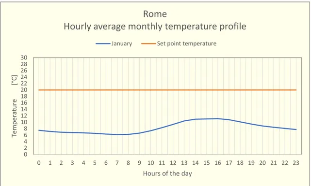
It is important to underline that ISO 13790 approach does not aim to obtain the exact amount of energy demand of the building. It is in fact a quasi-steady-state model: it has a good reliability for the heating energy need in winter period, which is often the most onerous component of the energy demand, but in summer the oscillation of the outside temperature produces a frequent inversion of the heat flow through the building envelope and the dependability of the quasi-steady-state model is heavily undermined.
4 EN 15316-1:2007 - Heating systems in buildings. Method for calculation of system energy requirements and system
efficiencies. Part 1: General 0 2 4 6 8 10 12 14 16 18 20 22 24 26 28 30 0 1 2 3 4 5 6 7 8 9 10 11 12 13 14 15 16 17 18 19 20 21 22 23 Temp er at ur e [°C]
Hours of the day
Rome
Hourly average monthly temperature profile
January Set point temperature
21 Figure 2 and Figure 3 are placed in Rome, so that the reader can understand the limits of a quasi-steady-state model. In winter the average temperature is constantly below the conventional heating set-point temperature (20 °C); on the other hand, this is no longer true in the cooling season, when the external temperature oscillates above and below the set point temperature (26°C) and the flow direction is more dynamic.
For this reason RetroSim is integrated with a dynamic building simulation. This part of the tool is destined to the differential calculation of the energy balance of the building with the components defined in Chapter 2.1, in the progression of every hour of the year. In this it can fix the mistake in the cooling evaluation, providing a more precise estimation of the energy demand. My program will make use of a substitutive version of the simulation backend, for the calculation of the energy demand of the existing layout and for the energy performances of the retrofit alternatives.
I decided to validate this approach through the comparison of its results with a reliable software coming from the experience and the technical knowledge in the field. This validation tool has been individuated in TRNSYS dynamic simulation. TRNSYS is a simulation program for energy engineering and building dynamic simulation, primarily for passive as well as active solar design, developed at the University of Madison-Wisconsin. The building and its plants are analysed through their main active components, describing, connecting and studying their dynamic performance. I used the software to make a comparison between the outputs coming from two different models:
- “Type 88 - Lumped capacitance building with internal gains”, which follows the assumptions employed in RetroSim and in my algorithm
- “Type 56: Multi-Zone Building”, the most sophisticated dynamic model inside the software. I tested a standard building in three different climates, in regard to understand and validate the behaviour of Heat4Cool model under all possible external conditions.
0 2 4 6 8 10 12 14 16 18 20 22 24 26 28 30 0 1 2 3 4 5 6 7 8 9 10 11 12 13 14 15 16 17 18 19 20 21 22 23 Temp er at ur e [°C]
Hours of the day
Rome
Hourly average monthly temperature profile
August Set point temperature
22
2.3 Description of the reference building
The building I simulated is the Reference Framework for System Simulations of the IEA SHC Task 44 / HPP Annex 38 (Figure 2.45), in three climates: warm in Athens, cold in Helsinki and Strasbourg as average continental climate.
Table 2.A - Measures of building external surfaces
Surface A B C D E
Net area [m2] 54.6 26.4 45.7 56.0 70.0
Table 2.B - The three different prototypes of building
Code Heat exchange area Air zone volume Infiltration rate Old Building SFH 100 394.3 m2 389.45 m3 0.4 V/h Reference Building SFH 45 409.8 m2 389.45 m3 0.2 V/h New Building SFH 15 420.8 m2 389.45 m3 0.1 V/h All of the three buildings are sharing the same geometry. Their main difference is in the insulation layer thickness, hence the heat load. The houses of Table 2.B are named SFH (Single-Family House) 15, 45 and 100.
- SFH15 represents an actual building envelope with very high energetic quality. It fits the Swiss Minergie-P (Minergie 2010) and German Passivhaus (Feist 2005) requirements;
- SFH45 elements are constructed, such that they are oriented at actual legal requirements or represent a renovated building with good thermal quality of the building envelope;
- SFH100 represents a non-renovated existing building.
The orientation is represented by the arrow indicating the North. The common geometrical structure of the buildings is fixed by inside measures, summarized in the Table 2.C.
5 R. Dott, M. Y. Haller, J. Ruschenburg, F. Ochs, J. Bony - The Reference Framework for System Simulations of the IEA SHC
Task 44 / HPP Annex 38. Part B: Buildings and Space Heat Load Figure 2.4- Building general view
23 The building is studied as one common thermal zone. Differently from the IEA work and my program, on TRNSYS internal walls and floors play an active role in the simulation (internal heat capacities). Simulation is based on external measurements in Table 2.A, no additional thermal bridges are considered.
Table 2.C - Constructive characteristics of the building
Layer s [m] ρ [kg/m3] [W/m∙K] λ [kJ/kg∙K] C U [W/m2∙K] SFH 15 SFH 45 SFH 100 SFH 15 SFH 45 SFH 100 External wall Inner plaster 0.015 0.015 0.015 1˙200 0.600 1.000 0.200 0.333 1.292 Brick 0.210 0.210 0.210 1˙380 0.700 1.000 EPS 0.200 0.120 0.040 17 0.040 0.700 Outer plaster 0.003 0.003 0.003 1˙800 0.700 1.000 Ground floor Wood 0.015 0.015 0.015 600 0.150 2.500 0.201 0.414 1.124 Flooring plaster 0.080 0.080 0.080 2˙000 1.400 1.000 Sound insulation 0.040 0.040 0.040 80 0.040 1.500 Concrete 0.150 0.150 0.150 2˙000 1.330 1.080 XPS 0.220 0.160 0.080 38 0.037 1.450 Roof ceiling Gypsum board 0.025 0.025 0.025 900 0.211 1.000 0.180 0.510 0.908 Plywood 0.015 0.015 0.015 300 0.081 2.500 Rockwool 0.200 0.160 0.040 60 0.036 1.030 Plywood 0.015 0.015 0.015 300 0.081 2.500
Int. wall Clinker 0.200 0.200 0.200 650 0.230 0.920 0.964 0.964 0.964
Table 2.D – Orientation and measure of the windows of the building
Orientation North South West East Total
Window area 3 m2 12 m2 4 m2 4 m2 23 m2
Table 2.E - Thermal and optical characteristic of the windows
Frame percentage Solar factor Transmittance
SFH 100 0.15 0.755 2.830 W/m2∙K
SFH 45 0.15 0.622 1.270 W/m2∙K
SFH 15 0.15 0.585 1.100 W/m2∙K
I used a total heat transfer coefficient hi=7.69 W/m2∙K to the inside and he=25.0 W/m2∙K to the outside (ambient).
24
Table 2.F - Resume of the global building parameters
SFH 100 - OLD BUILDING
Heat transfer coefficient 450 W/K
Heat capacitance 116˙000 kJ/K
SFH 45 - REFERENCE BUILDING
Heat transfer coefficient 160 W/K
Heat capacitance 99˙000 kJ/K
SFH 15 - NEW BUILDING
Heat transfer coefficient 90 W/K
Heat capacitance 120˙000 kJ/K
Internal gains are scheduled with the profiles in Table 2.G, with sensible heat production per person equal to 60 W and latent heat coming from a moisture hourly rate of 0.059 kg/pers.
Table 2.G - Profiles of the internal gains
Starting time Electricity gains [W] Occupants
0 105 4 1 55 4 2 55 4 3 55 4 4 55 4 5 55 4 6 392.5 2 7 457.5 3 8 420 2 9 55 0 10 55 0 11 250 1 12 55 3 13 120 2 14 120 1 15 120 0 16 120 0 17 170 1 18 170 2 19 615 2 20 420 4 21 420 3 22 442.5 4 23 355 4
25
2.4 Dynamic simulation of the reference building with TRNSYS models
The most valid method to model a building on TRNSYS is through the Type 56 - Multi-Zone Building, “models the thermal behaviour of a building having multiple thermal zones. The building description is read by this component from a set of external files. The files can be generated based on user supplied information by running the pre-processor program called TRNBuild.”6
Nevertheless, on TRNSYS exists also Type 88 - Lumped capacitance building with internal gains, “models a simple lumped capacitance single zone structure subject to internal gains. […] it neglects solar gains and assumes an overall U value for the entire structure. Its usefulness comes from the speed with which a building heating and/or cooling load can be added to a system simulation.” Its approach is very similar to the adopted one for the simulation tool, out of the fact that the project tool does not neglect the solar gains.
The final goal of Chapter 2 is the comparison of the outputs coming from an extensive al building envelope modelling, through the Type 56, with the ones from the simplified Type 88, adding the solar gains. The main approximation deals with the impact of the effective capacitance of the building: in Type 88 is equal to the theoretical capacity, merged in a single node, analysing the heat flow as a one-dimensional flux through the envelope; on the other hand, with Type 56 building thermal capacity is treated through a network of points.
Both models are simulated in the same TRNSYS file, through the architecture of Figure 2.5.
6 Solar Energy Laboratory, University of Madison-Wisconsin - TRNSYS 17 a TRaN sient S Ystem Simulation program -
Volume 4, Mathematical Reference
26 Figure 2.5 contains all the TRNSYS components (types) necessary to design the two aimed simulations. It follows a brief explanation of its various parts. For a more detailed account of the whole model, Annex II reports TRNSYS deck file for SFH 45 in Strasbourg; the other cases follow the same logic.
This layout was run for all the three building references (SFH100, SFH45 and SFH15) in the three climates (Strasbourg, Athens and Helsinki), defining it through “CLIMATE” (Type 15) and “Turn” calculator, where I evaluated the solar gains.
First, I designed the building with Type 88. It studies building behaviour merging its complexity into one single resistive-capacitive node: all the geometrical and constructive characteristics are summed into two parameters, the “Building loss coefficient” and the “Building capacitance”. These values are shown in Table 2.F for each of the three constructive typologies and I provided them through the calculator “Inputs”. Building’s passive component is finalized providing the internal gains quantity and profiles with “Occupancy” (Type 14a) and “Electricity” (Type 14d), as shown in Table 2.G.
Type 88’s HVAC plant is defined with an ideal system with infinite power, “T88_Equipment”. Its operation is governed through “Heating controller” and “Cooling controller” (Type 22), two iterative feedback controllers which compare the internal temperature with the seasonal set-point and set-back I provide with “Heating Setpoint” and “Cooling Setpoint” (Type 14). I adopted the standard values of 20°C for winter season and 26°C for summer.
I designed the same building with Type 56 - Multi-Zone Building. It models the building as network of elements, studying the thermodynamics of the building through the heat exchange between them. It is a much more sophisticated instrument for building energy modelling, but in the same time it was developed for this purpose so, through TRNBUILD extension, the building can be defined with a much more intuitive front-end. I show an example of this in Figure 2.6.
The reader is invited to observe I provided the exact same inputs I just illustrated also to this Type, which explains the tangle of connections between all the types in the global model.
27
2.5 Results and comments
In the next figures and tables I resume the main information coming from the comparative analysis. The complete collection of the output here analysed are presented in Annex III.
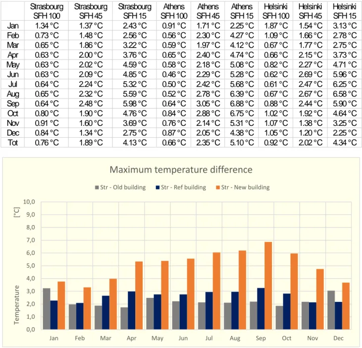
Table 2.H - Average monthly difference between Type 88 and Type 56 output temperature in free floating conditions
Strasbourg
SFH 100 Strasbourg SFH 45 Strasbourg SFH 15 SFH 100 Athens SFH 45 Athens SFH 15 Athens SFH 100 Helsinki Helsinki SFH 45 Helsinki SFH 15 Jan 1.34 °C 1.37 °C 2.43 °C 0.91 °C 1.71 °C 2.25 °C 1.87 °C 1.54 °C 3.13 °C Feb 0.73 °C 1.48 °C 2.56 °C 0.56 °C 2.30 °C 4.27 °C 1.09 °C 1.66 °C 2.78 °C Mar 0.65 °C 1.86 °C 3.22 °C 0.59 °C 1.97 °C 4.12 °C 0.67 °C 1.77 °C 2.75 °C Apr 0.63 °C 2.00 °C 3.76 °C 0.65 °C 2.40 °C 4.74 °C 0.66 °C 2.15 °C 3.73 °C May 0.63 °C 2.02 °C 4.59 °C 0.58 °C 2.18 °C 5.08 °C 0.82 °C 2.27 °C 4.71 °C Jun 0.63 °C 2.09 °C 4.85 °C 0.46 °C 2.29 °C 5.28 °C 0.62 °C 2.69 °C 5.96 °C Jul 0.64 °C 2.24 °C 5.32 °C 0.50 °C 2.42 °C 5.68 °C 0.61 °C 2.47 °C 6.25 °C Aug 0.65 °C 2.32 °C 5.59 °C 0.52 °C 2.78 °C 6.39 °C 0.67 °C 2.67 °C 6.58 °C Sep 0.64 °C 2.48 °C 5.98 °C 0.64 °C 3.05 °C 6.88 °C 0.88 °C 2.44 °C 5.90 °C Oct 0.80 °C 1.90 °C 4.76 °C 0.84 °C 2.88 °C 6.75 °C 1.02 °C 1.92 °C 4.64 °C Nov 0.91 °C 1.60 °C 3.69 °C 0.76 °C 2.14 °C 5.31 °C 1.07 °C 1.38 °C 3.25 °C Dec 0.84 °C 1.34 °C 2.75 °C 0.87 °C 2.05 °C 4.38 °C 1.05 °C 1.20 °C 2.25 °C Tot 0.76 °C 1.89 °C 4.13 °C 0.66 °C 2.35 °C 5.10 °C 0.92 °C 2.02 °C 4.34 °C
The first comparison is performed between the sole passive component of the building models, without any air-conditioning (free floating analysis).
It can observed that the difference between the two output temperatures goes up together with the increase of the technological performance of the building envelope. On the other hand, the discrepancy between average monthly values and its peaks is not very large, meaning that it is almost constant during the season and depends less on outdoor temperature variation. In SFH100 case, differences are very little and the peaks are concentrated at the start of the simulation, coming from the imposition of the boundary condition (Tinitial=20 °C). For this reason, these irregularities are not significative data.
0,0 1,0 2,0 3,0 4,0 5,0 6,0 7,0 8,0 9,0 10,0
Jan Feb Mar Apr May Jun Jul Aug Sep Oct Nov Dec
Temp er at ur e [°C]
Maximum temperature difference
Str - Old building Str - Ref building Str - New building
28 When I turn on the HVAC system, I assume it as ideal emitter, i.e. an air-conditioning system with infinite power that meets the user comfort during all the simulation time.
I obtain a temperature profile which is almost equal between the types, as desired. This means that I achieved a valid representation of the same building energetic configurations for the two different models. The achievement of this result will let me make a comparison of the energy performances.
Table 2.I, shown as example, was the one which gave the most irregular results I analysed, as observable in Figure 2.9.
Table 2.I - Temperature profiles in SFH 15 Athens
Avg temperature [°C] Max temperature [°C] Min temperature [°C] Exterior Type 88 Type 56 Exterior Type 88 Type 56 Exterior Type 88 Type 56 Jan 9.15 22.81 21.08 17.45 25.94 24.00 0.40 20.01 19.94 Feb 9.69 25.52 22.36 18.95 25.99 24.25 0.95 24.29 20.74 Mar 11.77 25.44 23.22 22.60 26.00 26.07 2.50 24.16 20.17 Apr 15.30 25.83 25.78 26.15 25.99 26.12 5.55 25.40 24.76 May 20.23 25.91 26.01 32.40 25.99 26.12 9.10 25.60 25.26 Jun 24.27 25.93 26.06 34.35 26.00 26.13 14.65 25.80 25.92 Jul 27.04 25.94 26.07 37.90 26.00 26.14 17.65 25.85 26.01 Aug 26.67 25.94 26.07 36.20 26.00 26.16 17.90 25.87 26.00 Sep 22.98 25.93 26.06 33.15 26.00 26.15 14.55 25.67 25.67 Oct 18.27 25.85 25.79 28.30 26.00 26.15 8.95 25.26 24.26 Nov 14.18 25.68 24.96 24.60 25.99 26.11 5.45 24.97 23.07 Dec 11.20 24.66 22.38 21.15 25.97 25.31 1.85 22.72 20.07 Total 17.56 25.45 24.66 37.90 26.00 26.16 0.40 20.01 19.94 Table 2.I is useful to demonstrate the substantial equivalence of the results: the annual average temperature difference between the two models is 0.79 °C, which becomes even smaller if analysed the maximum and minimum temperature difference, because they are direct consequence of the HVAC set-points.
For the same reason the biggest differences are confined into free-floating months, when nor heating or cooling is active. The maximum difference is 3.16°C between the types output in February, when less air-conditioning is necessary thanks to the heat capacity of the building.
This discrepancy is due to the fact that the dynamic energy balance written in Type 88 is: 𝑑𝑑𝑇𝑇 𝑑𝑑𝑒𝑒 = 𝑈𝑈∙𝐴𝐴 𝐶𝐶 ∙ (𝑇𝑇𝑖𝑖𝑖𝑖𝑒𝑒− 𝑇𝑇𝑒𝑒𝑒𝑒𝑒𝑒) + 𝑚𝑚̇𝑎𝑎,𝑣𝑣𝑣𝑣𝑣𝑣𝑣𝑣∙𝑐𝑐𝑝𝑝,𝑎𝑎 𝐶𝐶 ∙ (𝑇𝑇𝑣𝑣𝑒𝑒𝑖𝑖𝑒𝑒− 𝑇𝑇𝑒𝑒𝑒𝑒𝑒𝑒) + 𝑚𝑚̇𝑎𝑎,𝑖𝑖𝑣𝑣𝑖𝑖∙𝑐𝑐𝑝𝑝,𝑎𝑎 𝐶𝐶 ∙ �𝑇𝑇𝑖𝑖𝑖𝑖𝑖𝑖 − 𝑇𝑇𝑒𝑒𝑒𝑒𝑒𝑒� + ∑ 𝑄𝑄𝑔𝑔𝑎𝑎𝑖𝑖𝑣𝑣𝑔𝑔 𝐶𝐶 [K/s] As before, it refers to envelope transmission, air ventilation and infiltration and all thermal gains. The first derivative of temperature implies the thermal capacity involvement, which is lumped into a single parameter as the name of the type suggests.
Type 56 Multi-zone Building model provides a more efficient way to calculate the interaction between two or more zones by solving the coupled differential equations utilizing matrix inversion techniques. The effects of both short-wave and long-wave radiation exchange are accounted for with an area ratios method. The walls, ceilings, and floors are modelled according to the ASHRAE transfer function approach.7
7 Solar Energy Laboratory, University of Madison-Wisconsin - TRNSYS 17 a TRaN sient S Ystem Simulation program -
29 18,0 20,0 22,0 24,0 26,0 28,0
Jan Feb Mar Apr May Jun Jul Aug Sep Oct Nov Dec
Temp er at ur e [°C]
Strasbourg - SFH15
Type 88 - avg T Type 56 - avg T
18,0 20,0 22,0 24,0 26,0 28,0
Jan Feb Mar Apr May Jun Jul Aug Sep Oct Nov Dec
Temp er at ur e [°C]
Athens - SFH15
Type 88 - avg T Type 56 - avg T
18,0 20,0 22,0 24,0 26,0 28,0
Jan Feb Mar Apr May Jun Jul Aug Sep Oct Nov Dec
Temp er at ur e [°C]
Helsinki - SFH15
Type 88 - avg T Type 56 - avg T
Figure 2.8- Monthly average of the internal temperature for SFH15 in Strasbourg
Figure 2.9- Monthly average of the internal temperature for SFH15 in Athens
30 Figure 2.11 and Figure 2.12 summarize the HVAC demand output from the different case studies. The results are very similar in absolute values. The total demand in Table 2.J follows the expected trend, decreasing in more insulated buildings, but if divided into the seasonal demand, while the heating demand has a huge fall, the cooling demand increases. This phenomenon is repeated looking at lumped parameters model demand, because its internal temperature in free-floating is constantly higher than the output resulting from multi-nodal model of Type 56-B: therefore, its heating demand will be lower, but cooling demand higher.
If it is aimed to fix this discrepancy, a simple k-factor applied on building capacity C does not reach the bivalent effect aimed, because increasing/decreasing C it is obtained the same effect on both seasonal
0,0 5,0 10,0 15,0 20,0 25,0 30,0 35,0 40,0 45,0 50,0 55,0 60,0
STR SFH100 STR SFH45 STR SFH15 ATH SFH100 ATH SFH45 ATH SFH15 HEL SFH100 HEL SFH45 HEL SFH15
Ene rg y de m and [M W h]
Annual heating demand
Type 88 Type 56 0,0 5,0 10,0 15,0 20,0 25,0 30,0 35,0 40,0 45,0 50,0 55,0 60,0
STR SFH100 STR SFH45 STR SFH15 ATH SFH100 ATH SFH45 ATH SFH15 HEL SFH100 HEL SFH45 HEL SFH15
Ene rg y de m and [M W h]
Annual cooling demand
Type 88 Type 56
Figure 2.11 - Comparison of the annual heating demand
31 demands; the goal can be accomplished with a “seasonal” k-factor or through a corrective factor a posteriori on the heating/cooling demand.
Table 2.J - Comparison of the total energy demand
Type 88 Type 56 Type 88 vs Type 56
STR SFH100 34.81 MWh 36.85 MWh -5.52% STR SFH45 10.04 MWh 11.00 MWh -8.72% STR SFH15 6.71 MWh 6.01 MWh 11.67% ATH SFH100 17.46 MWh 18.52 MWh -5.73% ATH SFH45 8.88 MWh 7.72 MWh 15.10% ATH SFH15 10.06 MWh 6.73 MWh 49.58% HEL SFH100 55.59 MWh 58.35 MWh -4.73% HEL SFH45 16.75 MWh 18.58 MWh -9.87% HEL SFH15 9.79 MWh 10.12 MWh -3.26%
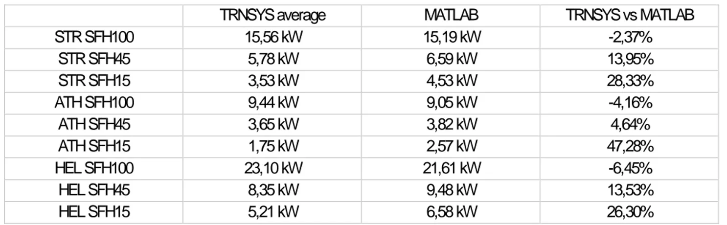
Talking about the relative error, it results limited in two of the three climates (Strasbourg and Helsinki) but in Athens, especially for case SFH 15, the relative difference is almost half of the total amount of energy demand (about 4 MWh/year). Unfortunately, lumped capacity model loses precision in conditions with high cooling demand, where the effect of thermal inertia is more valuable. This is compensated in terms of simplicity, flexibility and, above all, computational speed of the program. From the moment that my algorithm aims to provide the sizing of a large number of solutions for the estimation of the energy demand, with the objective of isolate the best solutions for a further simulation of their performance with a Multi-Criteria Decision Making, it is a defect that I accepted to leave. Furthermore, in terms of impact on the sizing this error is quasi-irrelevant:
- in Chapter 4.5 I will show that the sizing parameters for the generators will be affected in the order of maximum 2 kW;
- for the final Primary Energy demand estimation, the significative output is the relative comparison between existing layout and retrofit layouts. The possible imprecisions of the model will not affect it from the moment that I use the same computational model for all the HVAC system layouts. Moreover, making a global evaluation, the absolute difference between the outputs of the two energy models is acceptable for the purposes of the retrofitting tool, because the discrepancy is concentrated in the most modern building constructions which, in the same time, are not the main object of retrofit, while for older buildings the output equivalence is reliable, especially for heating period, where it is placed the largest part of energy demand and when the effect of internal heat capacity is less relevant on the thermal behaviour of the system.
32
3 The HVAC technologies contemplated by the algorithm
Heating, Ventilation and Air-Conditioning (HVAC) is managed with a large variety of systems, machineries and support elements. There is not an optimal solution conform to any type of building, because the performance depends on the dimensions of the heat flows involved and on the adaptation to different environments.
Chapter 3 introduces the state of the art of the retrofit solutions involved in the rehabilitation. It is present the most common HVAC equipment, together with some experimental machineries coming from the set for the project Heat4Cool.
3.1 The HVAC system types
Water-based system
The most ordinary HVAC system in residential buildings. Water is the heat carrier fluid that transfers heat from the generator to the emitters in the thermal zone.
In the past natural circulation systems were used, as for example the rain systems (top water distribution), and it was common the use of distribution with monotubes and heating bodies in series. Today, because of the evolution of pumps and plant technologies, the quasi-totality of water systems involves forced circulation plants, that is source plants (water distribution from below) with horizontal water distribution. The large majority of the hydraulic systems nowadays use also manifolds, each one supplying inlet water to its zone emitters.
Air-based system
These systems use as heat-transfer fluid for air conditioning the treated air in a centralized unit (called AHU, Air Handling Unit); air is distributed to the served rooms through a network of pipes. The air has the task of carrying out, at the same time, the control of the thermal load (sensible and latent) and the control of the quality of the ambient air. The origin of the air can be only external only, usually with heat recovery from the expelled air, or only internal, for delicate ambiences, or a mix of the two.
The major pros of these systems come out in applications on big buildings and large masses of air. Air emitters are frequent in northern countries, but they are generally adopted with a water-based system and in general in residential buildings it is infrequent to encounter such type of system, which on the other hand are much more frequent for the air-conditioning of public spaces and office buildings. At the same time, the layout of this plants is totally different from the others analysed, because it necessitates a detailed, specific design of the AHU.
For these reasons, I decided to not take in account this typology of HVAC system out of the cases where air is treated with a water HVAC system.
Electric system
Heat is provided though electric radiators which convert electric power into heating power for Joule effect. The efficiency of these systems, from an environmental point of view, is very low, because it consumes noble energy, such as electricity, for thermal purposes, without any intermediate process, wasting its potential. Because of the simplicity of installation, it was diffuse for the retrofit of very old buildings, before the growth of the eco-awareness, or in places with limited heating demand.
33 I decided to consider in the set of electric systems also the commonly called “air-conditioning” (A/C) for summer cooling in residential buildings, less commonly used also for heating in winter, which is in reality a system that uses a refrigerant fluid for a mono-split/multi-split fan-coils associated to an external chiller.
3.2 The emission subsystem
Heating elements are defined as “elements that yield the heat produced by a generator the environment; they are intended to yield heat in order to obtain, inside buildings, specific temperature conditions.”8 They are classified into two main typologies:
- Natural convection heating body: heating body that does not include a ventilator or a similar device for activate or move the air on the heating element
- Forced convection heating body: heating body that requires the action of a fan or similar device. Water radiators
The most frequent building heaters. They are heating bodies that emit heat by natural convection and irradiation. Radiators can be produced with different materials and forms (plate, column, tube).
The ideal functioning is with high water inlet temperature, because the yield decreases rapidly with lower water temperatures. They have mediocre speed of space heating and low uniformity of space heating. The regulation can be at zone control or at single element adjustment; they are silent elements and their average cost is very small.
Radiant floor
Radiant panels are heating bodies consisting in pipes placed behind the surfaces of the room to be heated. The heat is emitted in the environment partly by convection and, mainly, by radiation.
They can be:
- Radiant floor panels
- Wall-mounted radiant panels - Radiant ceiling panels
Generally, in residential buildings they are placed underfloor, so I referred to the sole underfloor heating. Their main feature is the zone heating uniformity, with heat that is mainly yield by irradiation. Figure 3.1, experimentally obtained, indicates that, in order to have ideal thermal conditions, it is necessary to maintain warm air near the floor and colder air on the ceiling. The radiant floor system allows to obtain a temperature curve close to the ideal one, thanks to the favourable position of the panels. It permits to keep the warm air near the floor and avoids the formation of hot air on the ceiling and cold on the floor, as happens on the contrary with traditional radiator or fan-coils systems.
The current trend prefers floor panels with surface temperature not lower than 19 °C and not higher than 28-29 ° C, to ensure comfort, respiratory and cardiovascular health. Compared to systems with
8 EN 442-2:2014 - Radiators and convectors. Part 1: Technical specifications and requirements
Figure 3.1 - Ideal temperature/height curve of the thermal comfort
34 traditional radiator heating elements, with underfloor heating it is possible to keep the ambient air at a lower temperature with the same thermal comfort conditions.
They are silent, but usually they are expensive. The working temperature of water is generally lower than the one for normal radiator, granting a possible source of energy saving.
Fan-coils
It is a heating body that emits heat though natural convection. A convector consists of, at least, the heating element and an outer casing that protects the ventilating unity. The ideal functioning of fan-coils is with low water inlet temperature, because it maximizes their yield. They have very good speed of space heating and high uniformity of space heating. As for radiators, the regulation can be a zone control or a single element adjustment. The noisiness is a sensible topic to be accurately designed; their average cost depends on the complexity of the unity but generally they can be not very expensive.
With water radiators and floor panels the cooling power obtained with cold water inlet is very poor and not-convenient. On the contrary, air emitting machineries can be coupled to mixed conditioning system for the emission of both heated or cooled air with equal efficacy, permitting the use of the same hydraulic system for the two purposes.
3.3 The generation subsystem
The heat generator is the component of the plant where the heat is produced, before it is transported to the terminals in the thermal zone. For summer cooling, the chillers produce the refrigerant power.
Heat generators
Traditional boiler
The traditional boiler is yet the most common heat generator in residential buildings. In a boiler two parts are distinguished:
- the burner, inside a combustion chamber, where combustion takes place
- the actual boiler, where the transmission of heat from the flame and from the combustion products to the heat transfer fluid is completed.
There is a series of auxiliary elements:
- the mantle with thermos-acoustic insulation;
- control tools (thermometers, manometers, pyrometers) and safety devices (thermostats, pressure switches, safety valves, temperature regulators, expansion vessel);
- fuel supply tubes; - fumes exhaust system. Condensing boiler
The technological evolution of the traditional boiler. It achieves very remarkable heating performances. In the traditional boiler they are summed various sources of heat dispersion in the different components of the water heating. The main innovation in condensing boiler is the possibility to manage condensation in exhaust fumes system, which gives the possibility to benefit of the the heat in exhaust fumes, lost in the combustion phase. This gives an extra-source of heat for the water pre-heating before it enters in the combustion chamber, producing a relevant increase in the efficiency of the boiler.
35 Figure 3.2 refers to:
A: traditional boiler at constant temperature B: modern boiler at constant temperature C: Temperature compensation boilers D: Condensing boiler
In most of the cases the boiler provides heated water for domestic use and building heating.; the exceptions are district heating or buildings without space heating.
Electric water heater
This electric device consumes electric energy to produce heated water. Heat is provided to water through an immersed electric resistance, which converts electric power into heating power, exploiting Joule effect. From the moment that it consumes noble energy, such as electricity, for a thermal utilization, it is a highly inefficient machine from an environmental point of view, but it is very simple to install and cheap. It can be used only for the production of domestic hot water.
Heat pump/chiller
With “Heat-pump/chillers” (HP) I group all the machines able to produce hot water up to the temperature of 50 °C and chilled water at 5 °C. Heat-pumps/chiller are thermal machines that work by transferring heat from a cold source to a hot one, able to do also the contrary (reversible cycle in Figure 3.3).
Figure 3.2 - Boiler efficiency in function of the load factor
36 Out of the usual electric HP, in the algorithm I considered three other types of HP, coming from Heat4Cool set:
- DC powered heat pump: an electrical reversible HP powered with Direct-Current (without inverter), so that it can be directly connected to a photovoltaic alimentation;
- Adsorption heat pump: an advanced HP which exploits the thermal properties of some specific materials, with an adsorbing cooling vessel and a desorbing heating vessel.
- Absorption heat pump: a reversible thermally driven HP. This is not contemplated in Heat4Cool project, but I added it for an ampler analysis.
In presence of low external temperatures, heat pumps are affected by a severe decrease of their heating power, whereas the heating demand of the building is higher. For this reason, it is common to provide a back-up boiler as support for the critic conditions.
Heat generation source
I consider four different types of fuel for the boiler. Each one will be related to a different PEf in function of their environmental impact. The deriving types of boilers are:
- Coal-burning boiler; - Oil-burning boiler; - Gas-burning boiler; - Biomass-burning boiler.
HPs are classified in function of the source used for the secondary circuit. This impacts on the COP (Coefficient of Performance) of the HP.
- Air source HP/Chiller; - Water source HP/Chiller; - Ground source HP/Chiller.
Renewable energy systems
They are added as possible additional source of energy, also two renewable generation systems. Solar thermal collectors
Solar thermal plant means a system that uses Sun as an energy source making it available in the form of thermal energy. Solar energy exploited by the solar thermal collectors can serve:
- to integrate the domestic hot water production - to integrate the heating system (combi-system) Photovoltaic panels
Photovoltaic panels, called more properly photovoltaic modules, allow to transform solar energy into electricity. The photovoltaic process of transforming the energy of the sun into electricity takes place in photovoltaic cells, generally in silicon, assembled in an appropriate way to constitute one the photovoltaic module.
The yield of the plant depends on the type of silicon constituting the cell, the precision in the design of the best slope/orientation of the modules, the ability in the design of the wires for the electrical connections and the quality of the electrical storage.
37
3.4 Thermal energy storage
Hot water tank
Buildings can be provided of water tank, used for storing hot water for space heating or domestic use. Indeed, water is a convenient and cheap heat storage medium because of its high specific heat capacity. An efficiently insulated tank can retain stored heat for days, reducing fuel costs for boilers, electric heaters or heat pumps. It is a necessaire element for the correct design of solar thermal plants, with high advantages especially in case it is used a stratified tank (Figure 3.4).
PCM tank
Currently, there are three major types of energy storage materials, including sensible, latent and thermochemical materials. Compared with sensible and thermo-chemical heat storage materials, phase change materials (PCM) have the advantage of high energy storage density and are able to maintain temperature (nearly) constant during the phase change process. Therefore, it has been widely used in many systems for storing thermal energy. 9
RetroSim takes in account heat batteries made from a formulation based on Sodium Acetate Trihydrate (SAT), solving the problems of segregation and corrosion, obtaining in the same time very compact modular solutions (Figure 3.5).
9 Y. Lia, G. Huanga, T. Xub, X. Liuc, H. Wub - Optimal design of PCM thermal storage tank and its application for winter
Figure 3.4 - Solar power available in function of the tank type