A new type of variable stiffness actuator using a continuously variable transmission : mechanical and control design

POLITECNICO DI MILANO

Laurea Magistrale in Ingegneria Meccanica

School of industrial and information Engineering

A new type of Variable Stiffness Actuator using a

Continuously Variable Transmission: mechanical

and control design

Relatore: Prof. Giuseppe Bucca

Correlatore: Ing. Alessio Prini

Thesis of:

Nader Riman

matricola 895619

Abstract

In this thesis, we design and control a new type of variable stiffness

actua-tor, an actuator that has a compliant element with the ability to change it’s

stiffness thanks to a continuously variable transmission. We will show that

by adjusting the intrinsic stiffness, through applying the optimal control

theory to get a task-specific trajectory and stiffness profile, it will result in

the best performance or highest efficiency the system can reach depending

on the required task. In this thesis, we will be applying an explosive

move-ment task to show the advantages in reaching higher velocities and higher

availability of power to use that a variable stiffness actuator can provide

over other classes of actuators such as series elastic actuator and the

classi-cal rigid actuator. An extensive comparison between the VSA and SEA will

be done to highlight how changing a stiffness can highly affect a system’s

performance. The control strategy adopted consits of a time-varying finite

horizon LQR that accounts for the non-linearities of the system and a low

level torque control which relies on position control thanks to the

propor-tional relation between deflection and force of the spring. Unfortunately,

experimental results are missing due to an unexpected tragedy that hit the

world (CoVid-19) and prevented physical work on this thesis.

Acknowledgements

My deepest gratitude goes to Ing. Alessio Prini for his continuous support

during this journey, I have learned a lot from him during this project and

I deeply appreciate the technical experience in design and control I have

gained from working under his supervision. Also, I would like to thank

Prof. Giuseppe Bucca for his follow-up and offering help and equipment in

critical situations. I would also like to express my gratitude to the CNR

team, Dr. Matteo Malosio for providing this opportunity and Ing. Tito

Dinon for his insight in mechanical design.

And most importantly, I would like to thank my family and friends for all

the much-needed emotional support that helped me stay motivated

through-out those 2 years and especially my parents for their excellent support for

me in the most vulnerable situations.

Contents

Abstract

1

Acknowledgements

3

1

Introduction

7

2

State of the art

13

2.1

Collaborative robots and safety issues

. . . .

13

2.1.1

Variable Impedance by Control . . . .

14

2.2

Serial Elastic Actuators . . . .

16

2.3

Variable Stiffness Actuators . . . .

17

2.3.1

Spring Preload . . . .

18

2.3.2

Changing ratio between load and spring . . . .

19

2.3.3

Changing physical properties of a spring . . . .

20

2.4

Continuously Variable Transmission

. . . .

21

3

System Dynamic model and Trajectory optimization

25

3.1

Ideal Model of the SEA and VSA

. . . .

26

3.1.1

SEA ideal Model . . . .

26

3.1.2

VSA ideal Model . . . .

27

3.2

Trajectory optimization and nonlinear programming . . . . .

29

3.2.1

Trajectory optimization . . . .

31

3.2.2

Cost Function . . . .

31

3.2.3

Parameter identification using optimal trajectory . . .

33

4

Mechanical Design & Components

35

4.1

Actuators & Sensors . . . .

36

4.2

Components . . . .

37

4.3

Mechanical Design procedure . . . .

41

4.3.1

Shaft design and sizing . . . .

41

4.4

Encountered Problems & Solutions . . . .

42

4.4.1

Bidirectional spring and preload system . . . .

42

5

Estimated real model & Control

46

5.1

Motor . . . .

46

5.1.1

SEA model . . . .

47

5.1.2

VSA Model . . . .

48

5.2

Control

. . . .

50

5.2.1

Low Level Control . . . .

50

5.2.2

High Level Control . . . .

52

5.3

Simulation . . . .

54

5.3.1

Results SEA

. . . .

55

5.3.2

Results VSA

. . . .

56

5.4

Final discussion . . . .

57

6

Comparison between VSA, SEA & a traditional rigid

actu-ator.

59

6.1

Performance comparison

. . . .

59

6.1.1

Rigid Actuator . . . .

60

6.1.2

Series Elastic Actuator . . . .

62

6.1.3

Variable Stiffness Actuator

. . . .

64

6.1.4

Discussion . . . .

67

6.2

Energy consumption comparison . . . .

68

6.2.1

Rigid actuator

. . . .

68

6.2.2

SEA . . . .

69

6.2.3

VSA . . . .

71

6.2.4

Discussion . . . .

72

Chapter 1

Introduction

Since the 60s and 70s, the first generation of robots have been used

in-tensively in the industrial sector to carry out different tasks. In modern

production plants, particularly in large assembly lines, robots have replaced

people in carrying out tasks that are generally really heavy or repetitive,

such as material handling of heavy parts in hazardous environments,

paint-ing tasks in car assembly lines, weldpaint-ing etc. This first generation consists

of robots able to perform sequences of operations in well defined

environ-ments and regardless of the presence of humans in the working area. For

this reason a lot of safety devices and procedures are used in order to avoid

the coexistence of humans and robots.

In modern years we are witnessing a paradigm shift in robotics from a

hierarchical one, where a robot is not able to react to the external

environ-ment perturbation, to a reactive paradigm, where the robot action changes

based on the external output in terms of force, vision or other external

measurements.

This change has made it possible to move onto a new generation of robots

able to react, on the basis of the control strategy chosen, to disturbances in

the external environment, including the human presence. This new

gener-ation of robots comprises the so called collaborative robot (cobot), a robot

designed to interact with humans in a shared space or to work safely in close

proximity.

The ability to react to changeable outdoor environments and to share

the work space with humans, without posing a danger to their safety, is

an indispensable feature also for other types of robots such as humanoids or

service robots that today appear on the market and in the world of research.

A well-known example is the one of the service robots produced by iRobot,

with their most famous product Roomba. Service robots are a perfect

sup-port for the medicinal services industry thanks to their precision, accuracy,

speed, flexibility and ability to work together with people. These robots are

presently being utilized by research facilities, in medical procedures,

reha-bilitation, support and improve the well being and lives of people around

us [1]. Revolutionary advancements can be made through the integration

of this innovative technology, which is significantly improving the recovery

and quality of life for patients [1].

Robotics is a field of engineering that involves several tracks of

engi-neering most importantly mechanical engiengi-neering and electronics, where it

is responsible of the hardware part (design and construction) and software

part (control and sensory feedback) that produces machines, with the goal

to substitute (or replicate) human actions, the end product is what we call

a Robot [2]. Industrial robots are the first type of robots[3] and in the

past they were mainly used for basic classical handling, assembly and

weld-ing tasks to a wide range of production applications such as quality control,

robot shaping, cutting, friction stir welding, folding and machining [4].

How-ever, the need for the coexistence of robots and people in the physical area,

by sharing the same workspace and actually interacting in a physical way,

introduces the key issue of guaranteeing of the well being to the person and

the robot’s safety. As far as industrial robots for the most part they require

secluding the workspace of the manipulators of that of the person by a door

or a barrier. Then again, an expanding interest is emerging in domestic and

industrial service robots, and in some situations even unavoidable physical

collaboration. Along these lines, a subsequent fundamental prerequisite is

to ensure safety for human users in normal activity mode just as in faulty

modes [5]. Humanoids are robots, nowadays relegated only to research areas,

designed to resemble humans, both functionally and aesthetically. This type

of robot can be thought of as a lab robot through which it is also possible

to face new technological challenges. The research and use of collaborative

service robots and humanoids have shown some evident technological limits

of the mechanical structures that today characterize modern robots. The

robots are in fact generally made up of a chain that can be closed or open

with rigid links moved by actuators placed at the joints. These actutors are

generally pneumatic, hydraulic or much more frequently electric [6], chosen

for their low cost and ease of use. The need for interaction with the

exter-nal environment is usually addressed by sensing the robot more frequently

through the use of force sensors or vision systems and a suitable control

sys-tem. The adoption of this type of structure has shown all its limitations over

the years in comparison with the animal exoskeletal system. The human

ex-oskeletal system in union with the central nervous system allows it to adapt

to a multitude of external environments but also to express performances

that do not seem attainable today with the classic mechatronic systems

de-veloped. Consider, for example, the ability of a modern footballer to kick a

ball at hundreds of km/h towards the goal, and after a few seconds to

col-lide safely with an opposing footballer; this enormous versatility in carrying

out the tasks is essentially linked to the elasticity of our exoskeletal system

and to the ability of the nervous system to properly exploit this elasticity.

For this reason, over the years there has been a growing interest in robotic

systems that somehow include elasticity in their structure, and at the same

time control strategies have been developed that can properly exploit the

mechanical characteristics of the robot to better perform different tasks.

In an initial phase, robotic research tried to delegate this elastic property

exclusively to appropriate control strategies, using particularly ready force

sensors and actuators. Even this strategy today shows limitations, due for

example to the impossibility of storing and releasing energy efficiently. The

scientific community therefore has started to create robotic structures

char-acterized by their intrinsic elasticity. Nowadays elasticity can be integrated

either through flexible links or through joints suitably designed to include

an elastic element. Elastic couplings in robotics are today divided into two

broad categories, the Serial Elastic Actuator (SEA) or the Variable

Stiff-ness Actuator (VSA). The latter can modify, generally through mechanical

reconfiguration, their elastic characteristics. This device, integrated into a

robot and assisted by appropriate control strategies, allows the achievement

of performances that approach those of the human musculoskeletal system

and are certainly part of the enabling technologies for the current and future

generation of robots. To date, this type of actuator is exclusively present in

the research field but does not find real uses in the industrial world, despite

the advantages indicated above. This is still due to the absence of a

pro-totype that provides the desired performance levels, the excessive cost and

the non-negligible weight for this type of systems in general.

Different research groups around the world are therefore trying to find

solutions to these application problems. This thesis aims to analyze some of

the problems affecting the actuators present in the literature today and to

in-vestigate in particular a solution already proposed at a theoretical level by a

Dutch research group which, however, does not find experimental references

at the moment. This study presents a prototype for a variable stiffness

ac-tuator using a continuously variable transmission (CVT). In order to reach

a variable stiffness, different factors can be changed, and one of them is

the gear ratio between the output link and the compliant element, where

a high gear ratio results in high stiffness and vice versa. The scope of this

thesis is to use a new type of bike CVT (figure1.1), and validating this

pro-totype consists of demonstrating the improvements of a VSA over a serial

elastic actuator by applying, in the presented case, an explosive movement

task which requires reaching high velocities in a small period. The data to

be collected will provide information about the efficiency and performance

gained in result of this device.

Figure 1.1: Sectioned CVT transmission.[7]

These kinds of robotic applications require a new kind of enabling

technolo-gies, the robots are mainly built from a series of actuators and links properly

joined together. Actuators are key enabling components for motion

genera-tion and control with properties that greatly impact the overall performance

of any mechanical systems. In general in robot construction the interest is

more on electric actuators,due to their high precision for position control

and great control flexibility [8]. The lack of suitable actuators has hindered

the development of high-performance machines with capacities equivalent to

people, particularly as for movement, safety and efficiency of animal beings

and humans. The functional and neuro-mechanical control performances

of natural muscle far surpasses that of mechanical instruments, with a key

contrast being the adaptable compliance or variable stiffness found in

or-ganic systems; this is very different from the performance of traditional stiff

electrical drives used in industrial robotics, which require accurate

reference-trajectory tracking [9]. However, in robotics applications it is often desired

to have varying characteristics of the actuator when it comes to speed and

force which are related through the stiffness of the actuator, and also in

achieving human-like locomotion therefore having a variable stiffness

actua-tor(VSA); an actuator that can inherently change the mechanical compliance

of the system it is in, has positive outcomes in terms of energy efficiency,

robustness against disturbances and similarity with human motions, we

ob-tain an actuator with different combinations of speeds, torques and stiffness.

The graph in figure(1.2) shows how the three are related. This device

in-Figure 1.2: 3D graph showing the working volume of a VSA with the output stiffness(z-axis) , output velocity (y-stiffness(z-axis) and output torque(x-stiffness(z-axis)[10]

creases performance and efficiency by optimizing the energy storage/release

of the spring and the stiffness.

In this work a detailed analysis of SEA and VSA actuators will be done,

focusing in particular on the CVT-VSA actuator. As already demonstrated

earlier, there are many features that make the use of an elastic actuation in

the construction of robots advantageous, and there are many applications

that can take advantage of these features. In order to demonstrate these

advantages of CVT-VSA we will focus on a particular application, i.e. the

launch of a basketball at the maximum distance. This simple application

allows to show how an elastic actuation can be exploited to improve the

performance of a robot during explosive movements.

In order to achieve this goal the work has been divided as follows. In

Chapter 2 the state of art will be introduced in order to make the reader

aware of the solutions currently present in the literature. In Chapter 3 it

will be shown how it is possible to model this type of actuator from the

me-chanical point of view. This phase is useful in order to correctly design all

the components that must then be used in the construction of the actuator,

considering the particular task chosen. In Chapter 4 the complete

mechani-cal design of CVT-VSA actuator will be shown with a brief introduction to

all the elements that make up the test setup. In chapter 4 a more refined

model will be shown. This phase will deviate from the work shown in

Chap-ter 2 for the choice of real parameChap-ters to be used in modeling, and for the

design of control strategies that best suit the task in question. Finally, in

Chapter 5, a comparison will be made in terms of performance between the

three configurations introduced here (rigid actuator, SEA, VSA) in order to

show the quality of the solutions adopted.

Chapter 2

State of the art

2.1

Collaborative robots and safety issues

Robots have been used in industry for more than 80 years and their job

is to replicate or substitute humans in a faster, safer and more efficient

way. But humans have been always secluded from being present in the same

workspace with a working robot due to safety issues[11]. Advancements in

technologies are continuously working on increasing the collaboration

be-tween the two. Collaborative robots are the type of robot coexisting and

physically cooperating with people, being capable of natural motions and

much closer to human performance than today’s robots. As the first rule

in Robotics by Isaac Asimov stated ”a robot may not injure a human

be-ing or, through inaction, allow a human bebe-ing to come to harm” [12] .This

sentence summarises that safety in robotics is the most important aspect.

This requires that robots with similar size and mass as humans also have

comparable power, strength, velocity and interaction compliance. However,

this goal cannot be easily reached with today’s technology, where robots

are very rigid for the sake of position precision [10]. When robots operate

in a dynamic environment, unexpected collision between robot and the

en-vironment are likely to occur. It is important that during these collisions,

both the robot and the object it is colliding with suffer as little damage as

possible. Especially when the collision happens with a human, in this case

the impact could lead to severe injury or fatal wound for the human.

Stan-dard industrial robot systems, due to their inertia, structure and process

forces, can pose serious hazards to humans [13]. Interest in robots allowing

physical interaction is highly increasing and, unlike their classical

counter-parts, they take into account for the hardware design, meaning the robot

cannot simply rely on computed trajectories, extra precautions are required.

Figure 2.1: Robot human interaction. [14]

In order for the robot to be dynamically aware of it’s environment, joints

with position control are not enough, the force on the joints has to be dealt

with by the robot also, for example a joint that’s trying to reach a reference

point by position control will try to reach that point without any

consider-ations. However, in a case where the joint is stuck with an obstacle during

the transition to the reference point, with position control, it will try it’s

full power to reach this point disregarding the stresses applied on it’s

sys-tem’s body/joint, but what if we have feedback on the force too, it would

prevent it from trying to overcome the obstacle to a point where it harms

itself or the obstacle (which could be a human) blocking the way. To tackle

this issue, a control approach is widely used to change the impedance of the

system using control.

2.1.1

Variable Impedance by Control

Figure 2.2: Force control vs Impedance control schematic [15]

Research on robot force control has boomed in the past thirty years.

Such high interest is motivated by the desire of providing robotic systems

with better sensory capabilities. Robots using force, touch, distance, and

visual feedback are expected to autonomously operate in unstructured

envi-ronments [16] . Force control is conveniently used with position control as a

hybrid Force/Position feedback [17], adding extra feedback for robots that

rely heavily on force feedback be it in Industrial applications (welding...) or

for interaction with humans. Impedance by control is a control approach

that imposes a dynamic behavior between end-effector and environment. It

is probably the most common control strategy to physically interact with

robots. It took high academic attention after the detailed works of Hogan

(1985) on Impedance Control and its implementation [18], where it imposes

a desired physical behavior with respect to external forces on the robot and

facilitates stable robot interactions with the environment by replicating soft

and passive contacts. For example, the robot is controlled to behave like

a second order mass spring damper system. Consequently, impedance

con-trol allows us to realize compliance of the robot by means of concon-trol. Force

control and impedance control are similar yet different: they both use force

feedback from a sensor but on the other hand, the force control has the

desired force as output and impedance control aims to change the

dynam-ics of the system to a desired impedance during contact [3]. Interaction

with a well-designed impedance-controlled robot is very robust and

intu-itive, disturbance response is also added to the commanded trajectory. A

major advantage of impedance control is that contact discontinuities do not

create such stability problems in these systems. Movements are mostly

real-ized with stiff actuation in combination with rigid high geared transmission

mechanisms [19]. It is used in many applications ranging from manipulators

performing tasks while in contact with the environment, humanoid robots

and a wide range of human machine interfaces ranging from simple desktop

haptic devices to rehabilitation robots and full body exoskeleton systems

[20].

However, a force sensor is required for impedance control. Such sensors are

known to be expensive in automation applications where high precision is

required. In order to track rapidly the force trajectories , the controller

bandwidth has to be high. It can be increased by increasing the gains,

how-ever, the gains cannot be increased beyond some limits, as the system will

become violently unstable [21]. Some problems may arise affecting the

sta-bility of the robot that relies on the feedback from the force sensor, using a

low pass filter to remove the high frequency noise decreases the bandwidth.

Therefore, the cut-off frequency should be chosen carefully. By using the

force sensor there’s a trade-off between stability of the system and the

re-sponse time.[22]

So in operations that are force controlled, the sensor dynamics have to be

taken into account in the design of the controller, due to them being of the

same order of magnitude of the whole system’s dynamics. The dynamics of

the sensor are not only influenced by the sensor itself but also by the system’s

dynamics, (higher loads carried at the sensor reduce its bandwidth)[23] and

filtering.

Albeit of its large usage in modern robots, the variable impedance control

lacks of an appropriate storage mechanism (such as a spring), much of the

energy is wasted and has to be continuously injected by active actuation.

The energy wasted is not negligible and can have high impact on the design

of mobile robots: for example a more energy efficient robot requires a small

battery which account for a part of the robot’s weight. And sometimes if

we have multiple robots in a plant, this difference in energy consumption

makes a big difference on a large scale.

In the next sections, we will talk about alternatives to impedance control

where we can take advantage of the energy that is lost by adding a

com-pliant element, between actuator and load, that can be exploited to store

energy and use it to increase the efficiency of the system and/or performance

depending on the application.

2.2

Serial Elastic Actuators

Traditional actuators are characterized by a very high stiffness between

ac-tuator and load, which makes it a perfect candidate for a precise position

control and stability but makes it a hazard in collaborative applications due

to the very high stiffness.

Figure 2.3: Serial Elastic Actuator

From the analysis of the problem related to stiff actuation, Pratt (1984)

broke the tradition of making the interface between the actuator and the

load as stiff as possible realizing many advantages could be exploited from

it. This new type of actuator, back then, was called Series elastic

actua-tor which consists of a spring between moactua-tor and load, therefore reducing

the high stiffness between the two. It presents several advantages such as,

greater shock tolerance, lower reflected inertia, more accurate and stable

force control, less inadvertent damage to the environment, and the capacity

for energy storage.[24]

Torque control in traditional actuators is a complex task, but since the

in-troduction of a spring between the motor and the load, it is proportional

to the relative difference between motor position and load position, so the

torque control transforms into position control. Moreover it is important

to consider the energy storage in the spring which can help increase the

efficiency of the system [25]. Despite the advantages deriving from the use

of SEA actuators, the introduction of an elastic element can lead to

disad-vantages mainly related to positioning errors and limited stiffness. For this

reason non-linear SEA can offer some solutions to the linear SEA problems.

The main characteristic in linear SEA models is the spring stiffness, which

is relatively proportional to the force bandwidth, so the higher the stiffness

the higher the force bandwidth. But there’s a trade off between high

band-width and impedance, the more we increase the stiffness, the impedance

also increases. On the other hand, for the same force bandwidth of a linear

SEA, a non-Linear SEA (non-constant stiffness) has a lower impedance for

example in the stiffening spring used in [26]. Non-Linear SEA such as the

HypoSEA which stretches the linear spring in a non-linear way resulting in

a high range of force control levels (4 orders of magnitude difference) from

torques less than 0.02 N.m, because the actuator starts with a low stiffness

which allows to obtain high resolution torques, to 120 Nm, because the final

stiffness is high therefore allowing high torques to be transmitted, [27] and

other actuators such as [28] where the actuator has a high stiffness that is

used for high precision position control until a high impact force is applied

on it where the force value exceeds a pre-determined threshold, at that point

the actuator has a low stiffness that is suitable for shock absorption. In this

case of non-linear SEA it was taken advantage of the high position precision

of rigid actuators and the shock absorption of a low stiffness device.[28]

Another way to exploit a compliant element and benefit from variation of

stiffness will be discussed in the next section about the prosperous Variable

stiffness actuators and their different designs and ways to manipulate the

stiffness of a system.

2.3

Variable Stiffness Actuators

Variable stiffness actuators (VSA) are a class of actuators that posses

multi-ple compliant elements and internal separately actuated degrees of freedom,

that allow the capability of changing their apparent output stiffness

indepen-dently from the actuator output position. The introduction of a mechanical

compliance introduces intrinsic, passive oscillatory behavior to the system,

but rather than trying to minimize this effect, the question arises if it can be

exploited for the actuation of periodic motions . the papers [29][30] allow us

to observe controlling a VSA to match their natural oscillations with a cyclic

motion pattern, embodying a desired behavior of the system while

minimiz-ing the energy input to the system. Variable stiffness actuators are serial

elastic actuators with the ability to change stiffness. In order to change the

stiffness,It can be done in three different ways shown in the (fig.2.4).

Figure 2.4: Different ways to change the stiffness [9]

In order to change the stiffness, the system is constituted of at least 2

motors (one for the actuator and one to change the stiffness).

2.3.1

Spring Preload

Figure 2.5: The LinArm device with the two pre-loaded non-linear springs in opposite direction to each other. [31]

In the Spring Preload category, the stiffness is adjusted by changing the

pretension or preload on the spring. Compared to the no load category, the

spring force is parallel to the spring displacement, hence, to change the

stiff-ness, energy has to be stored in the springs and may not be retrievable. To

overcome this a second spring with negative stiffness can be added, usually

resulting in a large passive angular deflection. One application is the

LIN-arm device for upper limb rehabilitation [31] where it uses two non-linear

springs(two linear springs in triangular form from each side, resulting in one

non-linear spring, 4 linear springs used in total) in parallel in order to obtain

a VSA, and this setup can only be done with nonlinear springs [9]. The two

springs have a resultant stiffness and equilibrium position controlled by two

motors working together. When the motors rotate in the same direction the

equilibrium position changes and when they rotate in opposite directions

the stiffness changes because of the non linearity.

2.3.2

Changing ratio between load and spring

The stiffness is adapted by changing the transmission ratio between the

output link and the spring element for example the mVSA-UT, a

miniatur-ized VSA, that can change its output stiffness independently of its output

position through varying the transmission ratio between the internal

me-chanical springs and the actuator output . As this design does not pre-load

the spring, theoretically at equilibrium, no energy is required to change the

stiffness since the force on the spring is orthogonal to the spring

displace-ment. In practice, friction has to be overcome and when the joint is not

at the equilibrium position energy is still needed to adjust the stiffness.

Nonetheless, energy consumption can be reduced. Another way to change

the ratio is the lever arm mechanism with variable pivot point used in the

CompAct-VSA.[32]

Figure 2.6: Schematic of the lever arm mechanism with variable pivot point. [32]

This class can be further divided into the following sub-classes:

• Lever length: the stiffness is adapted by controlling the configuration

of a lever mechanism.

• Nonlinear mechanical link: the stiffness is adapted by controlling the

properties of a nonlinear mechanical link.

• Continuously variable transmission: the stiffness is adapted by

con-trolling the transmission ratio of a continuously variable transmission.

2.3.3

Changing physical properties of a spring

Unlike the previous concepts, structure control modulates the effective

phys-ical structure of a spring to achieve variations in stiffness. To understand

the basic concept, consider the basic elasticity law:

F =

E × A × ∆L

L

= K∆L

F is the force, E the material modulus, A the cross-sectional area, L the

effective beam length, and ∆L is the extension. In this representation,

EA

L

represents the stiffness K. To control the structural stiffness, any of the three

parameters in this equation can be manipulated. E is a material property,

which cannot be controlled by a structural change, but for some materials, it

can be changed e.g. by changing the temperature[33]. Unfortunately, these

changes are very slow for such applications[9]. Another technique [34] is to

alter the cross section by having a beam with multiple sheets: the elasticity

of the beam is changed by applying a vacuum force to change the total cross

section of the beam. The stiffness can vary in a range of the number of sheets

squared.Other papers realized this using electrostatic force and pneumatic

force[35]. Other ways to change the stiffness by changing the active spring

length, by The Mechanical Impedance Adjuster [36], which contains a leaf

spring, connected to the joint by a wire and a pulley. The active length

of the spring is changed by a slider,the spring is held close to the structure

thanks to the roller on the slider. a feed screw is rotated by a motor, moving

the slider and therefore changing the stiffness.

In achieving energy efficient actuation with variable stiffness actuators, an

experiment was done by [37] comparing a SEA and a VSA by measuring the

final velocity of a hammer before impact. The results show that the SEA has

reached velocity around 300% higher than the motor’s maximum velocity

(due to taking advantage of the spring’s stored energy), then the VSA has

reached a maximum velocity 30% higher than the one reached by the SEA.

Another paper studies the energy consumption of another concept of

compli-ant actuators that exploits the dynamics by matching the compliance of the

actuator with the compliance of the system [32] . The desired motion should

be periodic in nature and the variable stiffness actuator should be efficient

in changing the apparent output stiffness. The first condition implies that

it is sensible to temporarily stored energy, because periodic motions have

an energy conserving property. The second condition ensures that using a

variable stiffness actuator is a sensible solution. Applications of VSA are

consequently found where robots must physically interact with an unknown

and dynamic environment for example the MACCEPA actuator was used

for Jumping robot[38], bipedal walking robot [39][40] therefore, the control

body actuator system must have abilities like :

• shock absorbing

• stiffness variation with constant load

• stiffness variation at constant position

• cyclic movements

• explosive movements

This thesis is inspired by the concept E2V2 introduced by Stramigioli [41]

in his paper ”A concept for a new Energy Efficient Actuator” that

concen-trates on the negative power produced by the Infinitely Variable

Transmis-sion combined with an elastic element, the concept is about introducing a

Continuously variable transmission which provides a smooth & continuous

change of the gear ratio between input and output and thus can be used to

change the apparent stiffness of the elastic element introduced independently

of the equilibrium position.

Figure 2.7: E2V2 Concept [41]

2.4

Continuously Variable Transmission

In the course of the most recent two decades, noteworthy research exertion

has been coordinated towards creating vehicle transmissions that reduce the

energy consumption of cars. This effort has been an immediate outcome of

the developing ecological concern forcing the orders of exhaust emissions

and increased vehicle efficiency on current vehicle producers and clients. A

Figure 2.8: Variable Diameter Pulley CVT [42]

continuously variable transmission (CVT) offers a continuum of gear

ra-tios between desired limits, which subsequently improves the efficiency and

dynamic execution of a vehicle by better coordinating the motor working

conditions to the variable driving scenarios[43] .

Figure 2.9: Toroidal CVT at limit positions [44]

A CVT is a growing car transmission innovation that offers a

contin-uum of gear proportions among high and low limits with less moving parts.

Thus, this improves the mileage and increasing performance of a vehicle

by permitting better coordinating of the motor working conditions to the

variable driving situations[43][45]. Today, CVTs are forcefully rivaling the

usual transmissions and car companies are as of now enthused about using

the different points of interest of a CVT in a generation vehicle. A

contin-uously variable transmission is likewise a promising power-train innovation

for future hybrid vehicles. So as to accomplish lower emissions and better

performance, it is important to catch and comprehend the itemized dynamic

connections in a CVT framework so productive controllers could be intended

to defeat the current losses and improve the mileage of a vehicle. There are

numerous sorts of CVTs, each having their very own attributes for instance

Variable-diameter pulleys (VDP) or Reeves drives, Toroidal or roller-based

continuously variable transmission (CVT) and Magnetic CVTs [45][46].

Be that as it may, belt and chain types are the most normally utilized

CVTs, among all, in car applications.

Figure 2.10: Nuvinci CVT [47]

The NuVinci CVP is a compact and high torque-density unit that uses

planetary spheres to offer continuously variable speed ratio control in

wide-ranging applications. When coupled with an advanced, yet economical

con-trol system to vary the speed ratio for optimal power-train operation, the

system shows benefits in overall vehicle performance.

Figure 2.11: a simplified cross section of the NuVinci CVP. A bank of balls (planets) is placed in a circular array around a central idler and in contact with separate input and output discs (or traction rings).[47]

Power comes through the input disc and is transmitted to the balls, then

to the output disc via traction at the rolling contact interface between the

balls and discs.

The speed ratio is defined by the tilt angle of the ball axis, which changes

the ratio of r

to r

, and thus the speed ratio . The result is the ability

to sweep the transmission through the entire ratio range smoothly, while

in motion or stopped. Choosing the right gear ratio at the right moment

in accordance with the torque input from the motor can be seen as an

optimization problem in order to obtain the desired control inputs.

Figure 2.12: presents the system kinematics, where riis the contact radius of the input

Chapter 3

System Dynamic model and

Trajectory optimization

In order to better investigate the mechanisms of operation of the VSA

ac-tuators and to better interpret the results obtained from subsequent

exper-imental tests, it is considered necessary to proceed by modeling the system.

As already mentioned, the objective of this work is the definition of an

experimental setup based on a new type of VSA actuator. To proceed with

the system sizing and commercial components identification, it must first

identify an application task. In this work we will focus on the ability of

VSAs to store and release energy. The store and release energy mechanism

is the same that is used by the muscles during the throwing of objects, as

in baseball the pitcher who pulls the ball towards the catcher.

Precisely for this reason we will initially focus on a basketball ball

throw-ing task. The goal will be to make the throw as efficient as possible or in

more basic terms to throw the ball as far as possible.

As the commercial components to be used and therefore their real

perfor-mances are not yet available, an ideal system will now be modeled hereafter

in this chapter, in which all the components do not show friction, efficiency

or delay. This ideal model is also useful for checking the suitability of the

tools to be used. In order to identify the quantities involved and proceed

with the sizing in addition to the model, it is also useful to consider the

trajectory that will be performed by the system. Starting from a careful

analysis of the state of the art [8] [48] it was verified how it is necessary to

use an optimization algorithm to identify the ideal trajectory for the launch.

This algorithm will be identified and validated in this chapter once the motor

power is identified.

Figure 3.1: Ball Throw task at different times, arrows represent Motor positions

3.1

Ideal Model of the SEA and VSA

The modeling must proceed with the analysis of the basic components and

the writing of the energetic terms for the formulation of the Lagrangian. In

order to initially simplify the modeling, but above all the identification of

the optimal trajectory, we start with the modeling of a SEA device. The

VSA model will be obtained by reformulating the equations considering an

ideal transmission between spring and end-effector. In the sequel the input

is considered as an ideal velocity source and no friction factors exist, to

further simplify the system. This further simplification can be made a priori

considering that the transfer function between motor torque and its speed

follows a higher dynamic than that of the system considered. Clearly this

transfer function will depend largely from the control parameters chosen for

this application, and this assumption will be verified later in this discussion.

3.1.1

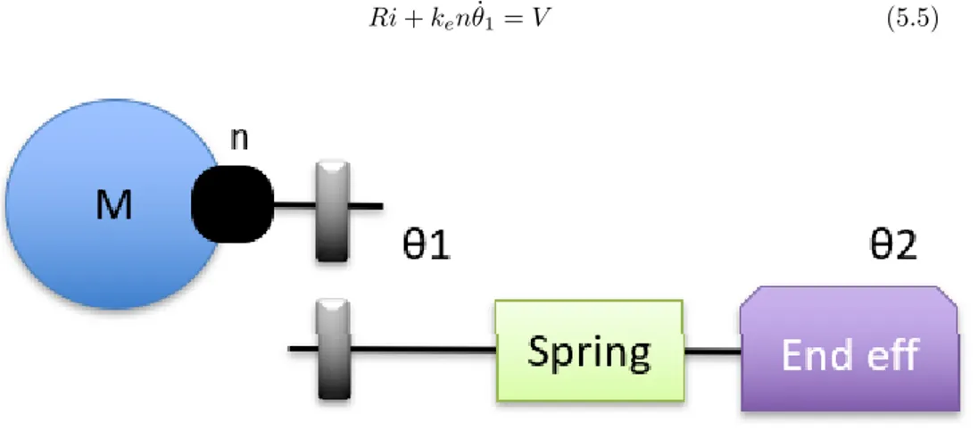
SEA ideal Model

Consider the model depicted in fig(3.2). Starting from this simple scheme

we can identify:

E

=

1

2

J

θ

˙

+

1

2

J

θ

˙

V =

1

2

Kθ

+

1

2

Kθ

− mglcosθ

Figure 3.2: SEA diagram

where m is the ball mass, l is the length of the arm and K the stiffness of

the spring.

that leads to:

d

dt

E

d ˙

θ

+

dV

dt

= u

For the sake of simplicity, and in order to reorganize the state variable the

same system could also be rewritten as:

θ

=

Z

0

˙

θ

dt

J

θ

¨

= K(θ

− θ

) − mglsin(θ

)

where J

is the inertia on the part of the end effector J

= J

+m∗(l+r

)

r

being the ball’s radius and J

is the rod’s inertia.

Considering the states:

x =







θ

θ

˙

θ







&

u = ˙

θ

3.1.2

VSA ideal Model

Figure 3.3: VSA diagram

In case of the VSA’s ideal model the motor is also considered a velocity

source. On the other hand, we will consider the CVT and the spring as one

entity as showed in fig (3.3) the stiffness of the combination of CVT and

spring resulting in the VSA is

(θ

−

) where (θ

−

)is the rotation of

the original spring. The variable stiffness

will be denoted as K

(t).

θ

=

R

0

θ

˙

dt

J

θ

¨

= K

(t)(θ

−

r

)

with the control inputs being u =

h ˙

θ

; K

(t)

i

.

J

q is the equivalent inertia for the system after the spring J

= J

/r

+ J

J

is the inertia between the spring and the CVT.

In an attempt to show one of the more important characteristic of VSA

with the respect to SEA, the graph 3.4 highlights the ideal available

stiff-ness range of each the two, the SEA is constrained by a line which represents

the stiffness

where φ is the deflection of the spring. The VSA is not

con-strained by a line rather by an area which is the main advantage of a VSA

device. To compare between the SEA and VSA, the torque of each device

is defined by the stiffness multiplied by the deflection. The deflection is

bounded between 0 and 1.5 rad for both device as it is a characteristic of

the spring. On the other hand the stiffness (K for SEA and K/r for VSA) is

different for both. Changing r the gear ratio in the VSA outputs different

stiffness as we can see in fig(3.4), the max stiffness line is when r is at its

minimum and the minimum stiffness line is when r is at it’s maximum.

Figure 3.4: Working region of an SEA & VSA

However, choosing which stiffness to apply at each time step is not

ran-domly done and is not a trivial task. In this specific task, it is an

optimiza-tion problem that requires the optimal stiffness at each time-step to ensure

the system is providing it’s highest performance or energy minimization

de-pending on the requirement. In other tasks it could be a specific stiffness

that is required by the user which nevertheless gives him a wide range of

stiffness choices.

3.2

Trajectory optimization and nonlinear

program-ming

Trajectory optimization is a collection of techniques that are used to find

open-loop solutions to an optimal control problem. In other words, the

so-lution to a trajectory optimization problem is a sequence of controls u*(t),

given as a function of time, that moves a system from a single initial state to

some final state. The resulting solution is open-loop, so it must be combined

with a stabilizing controller when applied to a real system [49]. Solving an

optimal control problem is not complete without NLP, it is a key element in

solving the optimal control problem. One of the algorithms to solve NLP is

the interior point method; a class of algorithms that solves constrained

opti-mization problems through solving sequence of approximate problems. They

are used to solve convex optimization problems. The basis of this method

re-stricts constraints into the objective function by creating a barrier function,

therefore restricting possible solutions to iterate only in the viable region,

which results in an efficient algorithm regarding time complexity [50].In

or-der to identify the quantities involved and proceed with the sizing in addition

to the model, it is also useful to consider the trajectory that will be

per-formed by the system. Starting from a careful analysis of the state of the art

[8][48] it was verified how it is necessary to use an optimization algorithm

to identify the ideal trajectory for the launch. This algorithm explained by

MathWorks ”NLP involves minimizing or maximizing a nonlinear objective

function subject to bound constraints, linear constraints, or nonlinear

con-straints, where the constraints can be inequalities or equalities. Example

problems in engineering include analyzing design trade offs, selecting

opti-mal designs, computing optiopti-mal trajectories, and portfolio optimization and

model calibration in computational finance”[51] . From Mathworks website

on nonlinear programming.

For a given state of the system x

the goal is to find a control law u(t, x)

that minimises the criterion [52] :

J (x

) = h(x(T )) +

Z

0

c(x(t), u(t)) dt

(3.1)

T being the final time of the task t ∈ [0 T ]

˙

x = f (t, x(t), u(t))

System Dynamics

c

≤ c(t, x(t), u(t)) ≤ c

Path constraints

b

≤ b(t

, t

, x(t

), x(t

)) ≤ b

Boundary Conditions

As will be further analyzed hereinafter, the optimization of the

trajec-tory for the thrown problem presented previously leads to the resolution of a

non-linear problem that cannot be solved analytically. This leads to the need

to find a numerical method for solving. Following a careful analysis,

differ-ent methods have been found in the literature and many libraries already

implemented in Matlab, the tool chosen for our analysis. The choice fell

on the optimization library developed by Kelly and presented in [49], where

multiple collocation methods can be chosen to optimize the given function.

In order to validate the chosen library and in order to choose the correct

col-location methods it was decide to start from the analysis presented in [48].

In this work different optimization problems are analyzed both analytically

and numerically. The simplest problem analyzed is composed by a simple

SEA without gravitational terms:

θ

=

Z

0

˙

θ

dt

J

θ

¨

= K(θ

− θ

)

In order to consider on 3.1 the constraints imposed by the dynamics of

the system it is convenient to introduce the Hamiltonian:

H(x(t), λ(t), u(t)) = c(x(t), u(t)) + λ

f (t, x(t), u(t))

To maximise the final velocity h(x(T )) =

q(T ) and c(x(t), u(t), t) = 0

˙

must be set. To solve the optimization problem the following system should

be considered:

˙

x =

∂H

∂λ

(3.2)

˙λ = −

∂H

∂x

(3.3)

As highlighted in [48] the resolution of this system leads to the typical

bang-bang control at the frequency equal to the resonance frequency of the system:

˙

θ

= ˙

θ

sgn(sin(ω(t − T )))

(3.4)

where ˙

θ

is the control while ˙

θ

is the maximum possible ˙

θ

value.

Considering this simple case many collocation methods have been tested

in order to compare the analytical exact solution with the numerical one.

Finally the Chebyshev orthogonal polynomials, an orthogonal collocation

method, has been chosen. Instead of having one segment in the trajectory,

this method divides it into multiple segments based on the paper done by

[53]. This is computationally fast and has a high precision for high

polyno-mial order and multiple number of segments. It has been decided to start

from a big mesh with low precision and kept iterating the solver with a more

precise mesh that relies on the results of the previous iteration. For the sake

of verifying the correctness of the solver, we compared the analytical

solu-tion to the solver’s solusolu-tion, a very high mesh refinement was also applied

to check how close can we get to the exact solution.

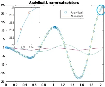
Figure 3.5: Analytical solution vs Numerical solution. the analytical solution is referred to in small circles, we can confirm that the solver is working.

3.2.1

Trajectory optimization

3.2.2

Cost Function

Our optimal trajectory is characterized by exploiting as much energy as

possible from the spring throughout the trajectory and to have almost no

energy stored prior to throwing the ball (which means the spring released

it’s previously stored energy). In our ball throwing task, an explosive

move-ment, the goal of the experiment is to maximize the distance thrown by the

actuator. Therefore, the algorithm has to find the best angle and highest

exit velocity of the ball at the moment of release. This experiment is done

in [30] with a different configuration of VSA, where they also were working

on maximizing distance thrown of a ball.

h(x(T )) is the terminal cost, and c(x(t), u(t, x(t))) is the running cost.

[52] The performance criterion which we previously discussed is formulated

into a cost function:

J

= −d(θ2(T ), ˙

θ

(T )) +

Z

−

1

2

w ∗ ||F (θ

, θ

)||

₊

1

2

R ∗ ||u||

_dt

_(3.5)

The throwing distance d is the terminal cost here and a ’-’ sign was

added in order to achieve the maximum instead of minimum. F being the

spring force , u is the motor effort and w & R are their weight numbers that

define how much priority each element of the latter is given, respectively.

The equation (3.6) is the terminal cost of the distance achieved from the

actuator, it can be better visualized in fig.(3.1).

d = x

(θ

) + ˙

x

(θ

, ˙

θ

)T

(θ

, ˙

θ

)

(3.6)

x

= l sin(θ

)

(3.7)

y

= −l cos(θ

)

(3.8)

T

=

1

g

(l cos(θ

) ˙

θ

+

q

(l cos(θ

) ˙

θ

)

+ 2g(y

− y

)

(3.9)

The problem becomes a ballistic equation where T

is the flight time

of the ball. x

/y

denote the horizontal and vertical positions of the ball,

respectively.

Constraints

Subject to the dynamics ˙

x = f (t, x, u) for SEA:

f (t, x, u) =















˙

θ

˙

θ

for VSA:

f (t, x, u) =















˙

θ

˙

θ

with

− ˙θ

≤ ˙θ

≤ ˙θ

Velocity control input limit

(θ

− θ

) − q < 0

Maximum spring rotation q

x

≤ x ≤ x

States boundaries

θ1max was limited to 3 rad/s

Maximum spring deflection (θ1− θ2) is 1.5 rad

θ2& θ1 are bounded by ±π₂

A low value for ˙θ1max was chosen since our goal is to highlight the improvement that the addition of a compliant element can give especially for under-powered actuators.

The spring constrained deflection is due to the design of the torsional spring. The gradient of this inequality path constraint is added in the path constraint with the goal to be as close as possible to a global minimum.

g(x) = [θ1− θ2− 1.5] ∇g(x)= [ ∂g(x) ∂t ; ∂g(x) ∂θ1 ; ∂g(x) ∂θ2 ; ∂g(x) ∂ ˙θ2 ; ∂g(x) ∂u ]

3.2.3

Parameter identification using optimal trajectory

The system was designed to use torsion springs as energy storage devices. One of the first obstacles is to identify the most suitable spring stiffness for our system. Not to forget other design constraints such as max rotation ◦, internal diameter, wire diameter, which are limited by spring manufacturing companies’ catalogues. The method used to identify the stiffness, is to iterate the optimal trajectory algo-rithm with different stiffnesses for each iteration, and check the overall performance of the system. We start by big steps at the first few rounds in order to detect the stiffness range of interest, and this range keeps diminishing until it reaches a suit-able resolution of stiffness. The criterion to differentiate between a suitsuit-able stiffness and non-suitable is the difference between ˙θ2and ˙θ1at time T ; it has to be positive

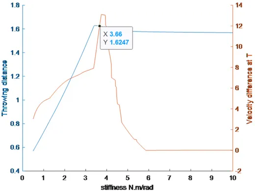
and high which is a sign that the spring energy was emptied or used prior to release of the ball (all the potential energy of the spring has been converted to kinetic energy), and another criterion the maximum throwing distance reached which is the terminal goal of our cost function (at the same time taking into account the other parameters mentioned previously for feasibility). The graph 3.6 shows the throwing distance increase proportionally with the stiffness at low values, which show the spring is exploited to the maximum constrained by the motor torque and the maximum allowable spring rotation, until it reaches a maximum point, which is the region containing the optimal stiffness value for the relevant application.

Chapter 4

Mechanical Design &

Components

The work shown up to here has dealt with identifying open robotics problem, iden-tifying solutions to overcome these problems and ideniden-tifying a reference task to experience the advantages of VSA and the proposed technological solution. Some simple models were also presented in order to give to the reader a first contact with the mechanical solution and to identify the main characteristics useful to face the design and sizing of a new setup. Now a new setup will be presented. This setup with a goal to experimentally test the advantages of the VSA-CVT solution. For this purpose in Figure 4.1 the mechanical scheme taken from the CAD model of the new setup is presented. A schematic list of the components used is also presented in the caption. As represented the setup in constituted by a gear-motor system connected by a pulley-belt system to a particular bidirectional elastic ele-ment. In turn this is connected to the CVT system, already presented in Chapter 2 and properly modified for this scope.Finally, the output shaft is connected to a sort of end-effector, able to grasp and release a basket ball, the ballistic object. Hereinafter, this work will go into detail of every component in order to better explain the reasons for the choices made and the changes made to the individual components.

Figure 4.1: 1.Motor 2.Motor Cup holder 3.Motor-shaft coupler 4.Belt-Pulley system 5.Encoder & holder 6.Torsional spring 7.Spring preload mechanism 8.Bearing & housing 9.Shaft Coupler 10.Force sensor 11.CVT 12.Stepper motor & belt-pulley 13.Ball throw mechanism

4.1

Actuators & Sensors

The motor that was used is a Low Voltage brushless servo motor is a SC05DBK from LS mecapion with a planetary gearhead (15:1) and an optical encoder attached to it’s back end, which will be used to have position feedback. The table (4.1)shows the motor characteristics.

Table 4.1: Motor Characteristics

Nominal Power (W)

450

Max RPM

5000

Nominal Torque (N.m)

1.43

Max Torque (N.m)

4.25

Velocity constant k

(V/RPM)

9.8

Torque constant k

(N.m/A)

0.157

Gear Ratio

15:1

Encoder (ppr)

2500

Figure 4.3: CVT gear change mechanism

Figure 4.4: CVT rolling spheres along with their arms

Therefore, with the addition of the gearhead that has an efficiency of 90% at the rated torque[58] the nominal output torque is around 19N.m and the max Velocity is 330RPM.

As will be shown below, in order to complete the task already shown in the previous chapter, it is necessary to carry out a so-called low-level control on the motor. As occurs in almost all automatic applications, this occurs through a feedback control of the kinematic or dynamic parameters. In this particular case, this control is entrusted to a commercial controller (Elmo Gold Cello) capable of carrying out both torque, speed and position controls on the motor. Communication with a central controller will take place via an EtherCat fieldbus. To make sure the position control of the spring ends (θ1and θ2) is resulting in the correct torque estimation, a

rotational force sensor (fig4.12) Burster 86-2477 is used for validation.// In addition to the motor’s encoder, two encoders (” RE30E-500-213-1”) from Copal electronics with 500 ppr are attached on both ends of the CVT. one is attached on the extremity of the shaft before the CVT and the other is attached at the extremity of the output shaft near the end effector shown in (Fig.4.1 element number 5. The reason for choosing two encoders, whereas for the feedback purpose the required amount is just one, is to validate that the CVT is providing the requested gear ratio and to verify and measure eventually the slip through the CVT. The encoder attached to the motor and the end effector encoder are the feedback that is going to be used in the control of the system, and all other sensors are for validation.

4.2

Components

CVT

The CVT presented in this section is the same already shown in the Chapter 2. The CVT changes it’s gear ratio by rotating the gear mechanism (fig4.3) that is connected with the rolling spheres (fig.4.4). The gear change occurs when the spheres connecting the input and output of the CVT change their relative rotational axis, which is equivalent to changing the radius of the ball, this shift creates a difference between the rotating radius on the input side and the output side.

Figure 4.5: The components of the CVT from one side

Figure 4.6: The CVT freewheel

Figure 4.7: The CVT coupling

End effector Ball throw mechanism

The ball throwing mechanism having two suction cups to keep the ball attached to the arm during the experiment and abort the suction in the exact time of the launch. The suction cups 7320500000 from Aventics (fig.4.8) were installed in the position opposite to the tangential force shown in (fig.4.10) because referring to the graph in (fig.4.9) the centrifugal (or radial) force is proportional to the square of the velocity on the other hand the tangential force is proportional to the acceleration of the end effector, therefore they were installed in the tangential direction to guarantee holding the non-negligible basketball at all time of the task. The body of the end effector was chosen to be able to withstand the forces from the ball and have a minimal impact on the dynamics of the end effector.

Figure 4.8: Suction cup

Figure 4.9: Torsional and centrifugal forces on the end effector Figure 4.10: End effector

Figure 4.11: Bearing & housing Figure 4.12: Rotational force sensor

Bearings and couplers

The bearings and couplers used to join together the sections of the shaft are com-mercial. Bearings were chosen according to suitable diameter, working rpm and forces applied to it (fig4.11). The couplers (”721.25.3232”) from Huco were chosen according to their diameter and nominal torque.

Torsional Springs

The elastic element is composed by a quite complex mechanical system. Tt is mainly composed by two helical torsion springs. The spring stiffness optimization was done in the previous chapter resulted in specific characteristics of the springs. Unfortunately, in the real world parameters are most of the time not available as precisely needed, so the closest model to what was obtained in the results should be chosen. The torsional spring that was chosen is ”G.255.400.0950” from Vanel and has very close parameters to the ideal one.

Belt and Pulley

The Belt and pulley used between motor and the system are:

500 mm belt (10 / T5 / 500 SS) from Contitech and two 36 teeth pulleys with 5 mm pitch (286-5708) from RS-PRO. A belt tensioner was taken into consideration but it was not included in the CAD model.

The synchronous belt and pulley system was used because it was the most con-venient system for the design that could transmit high torque. The load of the belt and pulley was calculated based on the max torque in the system, the pulley diameter and the belt’s max load.

Stepper motor

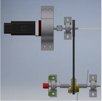
A Nema 16 stepper motor with a belt and pulley is used to change the gear ratio of the CVT, an alternative to the classical bicycle rotational gear change by hand. Stepper motor turned out to be the most useful choice for this particular appli-cation. The absence of feedback sensors makes this type of motor easy and cheap

to manage. The only problem to be addressed in practice is the need to refer the current position of the motor with the real transmission ratio. In this sense, the redundant use of the position sensors upstream and downstream of the CVT, help in this scope.

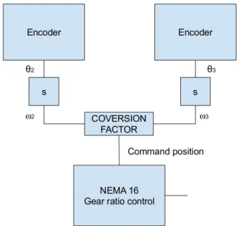
Figure 4.13: Gear feedback system. θ2 represents the position before the CVT, while

ω2being it’s derivative. The subscribe 3 represent position and velocity after the CVT.

The conversion factor represents the transform from gear ratio to motor position

4.3

Mechanical Design procedure

4.3.1

Shaft design and sizing

The maximum torque the motor can transmit is 19Nm, but in the task the max-imum torque reached is around 6Nm. However to be conservative, a safety factor of 2 was used when considering the torque, in case something goes wrong while experimenting so the system doesn’t fail. Two materials were considered for the shaft, Aluminum and low carbon Steel with a maximum shear stress of 50 Mpa and 200 Mpa respectively.

Since the major stress on the shaft is due to the torque by the motor, it was the only factor considered, however the diameter will be increased a bit to account for other factors.

τ = T ∗ c

π/2 ∗ c4 (4.1)

Where T is the torque, τ is the stress and c is the radius of the shaft.

The minimum shaft diameter, accounting for torsional shear stress only, for Alu-minum is 11.5 mm and 7 mm for Steel. However, larger diameters are considered