Independent Component Analysis of GPS time series in the Altotiberina fault region in the Northern Apennines (Italy)

Alma Mater Studiorum · Universit`

a di Bologna

Scuola di Scienze

Corso di Laurea Magistrale in Fisica del Sistema Terra

TITOLO TESI

Relatore:

Prof./Dott. Nome Cognome

Correlatore: (eventuale)

Prof./Dott. Nome Cognome

Presentata da:

Nome Cognome

Sessione

I / II / III

Anno Accademico

201*/201*

Independent Component Analysis of GPS time

series in the Altotiberina fault region in the

Northern Apennines (Italy)

Prof. Maria Elina Belardinelli

Correlatore:

Relatore:

Dott. Enrico Serpelloni Dott. Adriano Gualandi

Presentata da:

Cristina Nichele II

Sessione II

Anno Accademico 2015/2016

Correlatori:

i

Abstract

L'analisi delle componenti indipendenti (Independent Component Analysis, ICA) è una tecnica di statistica multivariata che consente di scomporre un segnale complesso in un certo numero di componenti, tra loro statisticamente indipendenti, che rappresentano le principali sorgenti di quel segnale. La tecnica ICA è stata applicata a serie temporali di spostamento GPS relative a 30 stazioni localizzate nell'Alta Valle del Tevere, nell'Appennino settentrionale. In quest'area, una faglia normale a basso angolo di immersione (circa 15°), faglia Altotiberina (Altotiberina fault, ATF), risulta attiva e responsabile di microsismicità (ML< 3), nonostante la teoria di Anderson sulla fagliazione

affermi che non dovrebbe esserci scorrimento su faglie normali di questo tipo. L'interesse per l'ATF è inoltre dovuto al suo potenziale sismogenetico: un evento che dovesse attivare l'intera faglia (lunga circa 70 km) avrebbe infatti magnitudo intorno a 7. Per questo motivo la zona è monitorata da reti multiparametriche (sismiche, geodetiche, geochimiche) che registrano dati in maniera continuativa, rendendo possibile l’individuazione anche di piccoli segnali di deformazione transiente.

Applicando la ICA alle serie temporali GPS si ottiene una scomposizione del segnale in 4 componenti indipendenti. L’analisi di queste componenti ha portato all’individuazione di correlazioni con serie temporali di piovosità, temperatura e sismicità. Una delle componenti, che presenta un segnale transiente di origine tettonica, è stata poi invertita per determinare la distribuzione dello scorrimento su piani di faglia noti. Il momento sismico associato allo scorrimento sulle faglie risulta maggiore del momento sismico associato ai terremoti registrati nell'area, suggerendo quindi che una parte dello scorrimento sia dovuto a movimenti asismici.

iii

Contents

Introduction

v

1. The Altotiberina fault

7

1.1 Geological and tectonic framework ………... 8

1.1.1 Low angle normal faults, faults mechanics and seismicity …………. 11

1.2 The Altotiberina Near Fault Observatory (TABOO) ………. 12

2. GPS data and surface displacements

15

2.1 Data: GPS time series ………. 15

2.1.1 GPS data processing and position time series ……….… 16

2.2 Strain-rates and time-series of strain ……….…. 19

3. Independent Component Analysis (ICA) on GPS time series

23

3.1 Independent Component Analysis (ICA): basic principles ………. 24

3.1.1 The ICAIM software ………... 26

3.1.2 Determining the number of useful components ………... 28

3.2 ICA decomposition of GPS signals ………..…. 29

3.3 Final decomposition for the ATF ………...… 29

4. Analysis of the independent components

35

4.1 First component ………... 35

4.1.1 Correlation with rainfall ……….. 37

4.2 Second component ………. 38

4.2.1 Correlation with the seismic catalog ………...…… 39

iv

4.2.1.2 Results ………... 44 4.3 Fourth component ……….. 51 4.3.1 Correlation with seismicity ……….… 53

5. Inversion of the fourth independent component

55

5.1 Inversion theory ………... 55 5.2 Inversion in ICAIM ………... 57 5.3 Results ……….... 59

Conclusions

69

Bibliography

73

Acknowledgements

85

v

Introduction

The Altotiberina fault (ATF) is a low angle (15°-25° east-dipping) normal fault (LANF) located in the Umbria-Marche sector of the northern Apennines of Italy. Based on the Andersonian [Anderson, 1951] theory of faulting, as typically applied to upper continental crust, normal faults should be precluded to slip at low (<30°) dip angles; nevertheless many field-based studies [Lister and Davis, 1989, Axen, 1999] and the interpretation of seismic reflection profiles [e.g. Floyd et al., 2001] indicate that LANFs can be tectonically active and generate earthquakes [Rigo et al., 1996, Abers et al., 1997,

Axen, 1999, Chiaraluce et al., 2007]. Despite the fact that the ATF is thought to be the

main structure accommodating extension in the region, no large earthquakes have been recorded along the ATF plane since 2 Ka [Rovida et al., 2016]. However Chiaraluce et al. [2014] pointed out that based on the size of the fault, an event activating the entire ATF should be around Mw 7. Recently, using a dense network of Global Positioning System (GPS) stations, Anderlini et al. [2016] studied the present-day crustal deformation of this area, finding that the ATF plays an important role in accommodating the SW-NE extension in the Northern Apennines being the largest part of the fault surface creeping at a rate of (1.7±0.3 mm/yr). In order to monitor this region, a research infrastructure (TABOO, The

Altotiberina Near Fault Observatory), recording high-resolution multiparametric data

(seismic, geochemical, geodetic), has been built in 2010. The presence of such a dense network makes it possible to detect even weak transient signals such as slow slip events.

In this thesis I analyze surface displacement time series of 30 GPS stations located around the Altotiberina fault, by means of a multivariate statistical technique called Independent Component Analysis (ICA). ICA provides a way to solve Blind Source

vi

Separation (BSS) problems, finding the sources that are superimposed in a mixed signal. When applied to GPS time series, ICA permits to decompose them into a proper number of components, statistically independent one from the others, which represent the major kinds of variation of displacement as a function of time in the investigated region. The aim of this thesis is to find the best decomposition for the dataset and propose a physical explanation for each IC. Further analyses, aimed at a better description of the physical processes at the base of the highlighted deformation signals, are also pursued using the Independent Component Analysis-based Inversion Method (ICAIM) code developed at the Istituto Nazionale di Geofisica e Vulcanologia (INGV) and University of Bologna [Gualandi, 2015] as an extension of the PCAIM (Principal Component Analysis-based Inversion Method) code [Kositsky and Avouac, 2010], developed at the California Institute of Technology (CalTech). The code allows us also to invert one or more IC in order to model the slip distribution on a predetermined fault geometry.

Chapter 1 contains a description of the Altotiberina fault (ATF) and the geological and tectonic framework of the northern Apennines, where the fault is located.

In Chapter 2, after briefly describing how GPS time series are obtained, I show the results of a strain analysis performed in the ATF region to determine the evolution of the dilatation with time.

The basic principles of the Independent Component Analysis (ICA) technique are exposed in Chapter 3, where the ICAIM code is described. I also show the final decomposition for the 30 GPS stations that compose the dataset. Each IC is then described in Chapter 4, where hypothesis on the sources of those signals are proposed based on the observed correlations between the temporal part of 3 ICs (one is thought to mainly reproduce noise) and time series of cumulated rainfall, mean air temperature and cumulative number of earthquakes.

Finally, in Chapter 5 I present the results of an inversion of the fourth IC, performed in order to determine a model for the slip distribution on rectangular fault planes.

7

1. The Altotiberina fault

The Altotiberina fault (ATF) is a ~60 km long, NNW-trending, east-dipping (15°-25°) low angle normal fault (LANF). It reaches a depth of approximately 12 km, which suggests a downdip extent of 35 km or more [Finocchio et al., 2013]. It is clearly imaged in the CROP03 deep seismic reflection profile [Barchi et al., 1998] and located in the Upper Tiber Valley at the Tuscany–Umbria–Marche regions boundary within the northern Apennines, as shown in Figure 1.1.

The existence of this structure is documented in geological [e.g., Brozzetti 1995,

Brozzetti et al., 2000] and geophysical data [e.g., Mirabella et al., 2011], as well as rather

well imaged by the associated microseismicity, even though the Andersonian [Anderson, 1951] theory of faulting, as typically applied to the upper crust, precludes normal faults from slipping at low (<30°) dip angles. GPS data also documented contemporary extension that is likely accommodated by creeping on the ATF [Hreinsdottir and Bennett, 2009].

The geophysical interest for this area, mainly due to the fact that, based on the size of the fault, medium to large earthquakes could nucleate along the fault plane, moved the scientific community to build a research infrastructure (TABOO, The Altotiberina Near

8

1.1 Geological and tectonic framework

The northern Apennines consist of a NE-verging thrust and fold belt, formed as a consequence of the collision between the Adriatic microplate and the European continental margin (Sardinia–Corsica block) [Collettini and Barchi, 2002].

Geologically, the region comprises a cover sequence of continental margin sedimentary rocks deposited upon a Paleozoic metamorphic basement [Chiaraluce et al., 2007].

The study area represents a transitional zone, being located just on the border between the inner extensional Tyrrhenian domain and the outer compressional Adriatic

Figure 1.1: Maps of the Northern Apennines region. In red the trace of the Altotiberina fault and of synthetic and antithetic faults obtained from geological survey.

9 domain [Collettini and Barchi, 2002].

The extensional tectonics of the Northern Apennines started in the eastern part of Corsica in the Lower Miocene, then moved eastward, reaching the Umbria region in the Upper Pliocene [Ambrosetti et al., 1978; Jolivet et al., 1998]: the Altotiberina fault has accumulated 2 km of displacement over the past 2 Ma [Vadacca et al., 2014]. This region is still extending at a rate of about 3 mm/yr [Serpelloni et al., 2005, D’Agostino et al., 2009]. Recent studies provides more detailed pictures of both present-day strain rates and fault kinematics. Anderlini et al. [2016] showed that ~1 mm/yr of this SW-NE extension is accommodated in the inner (Tyrrhenian) sector of the study area, while ~2 mm/yr are accommodated by activity of the Altotiberina fault and of its antithetic fault system (see Figure 1.2a). The area of maximum extension, concentrated across a 30-40 km wide zone, coincides with the area of the strongest seismic moment release [D'Agostino et al., 2009]. As shown in Anderlini et al. [2016] (Figure 1.2b) the strain-rate value in this sector is ~0.67x10-7 yr-1 of NE-SW oriented extension and it slows down going eastward and westward. The strain-rate calculated in this work (Chapter 2) for the ATF region is consistent with the value estimated in Anderlini et al. [2016].

In the past 20 years, three main seismic sequences have occurred within the hanging-wall of the ATF: the 1984 Gubbio sequence (Mw 5.1), the 1997 Colfiorito multiple-main-shock sequence (Mw 6.0, 5.7 and 5.6), and the 1998 Gualdo Tadino (Mw 5.1) sequence [Barba and Basili, 2000, Boncio and Lavecchia, 2000, Boncio et al., 2000]. Up to now, instead, only micro-earthquakes (ML<3.0) have been observed to continuously nucleate along the ATF plane [Chiaraluce et al., 2007, De Luca et al., 2009], mostly in its southern portion [Piccinini et al., 2003], at high and constant rate (r = 7.3×10−4 earthquakes day-1 km-2) [Chiaraluce et al., 2009]. The lack of microseismicity in the 20 km long northern section of the ATF suggests the existence of a locked portion along the ATF plane, which may be considered a seismic gap and thus may be hazardous [Piccinini et al., 2003]. Anderlini et al. [2016] found that the ATF is mainly locked down to a depth of 4-5 km, while the largest part of the fault surface is creeping at a rate of ~1.7 mm/yr except for a dipper asperity at 7-10 km of depth. The creeping portion correlates with the relocated microseismicity.

10

The deformation associated with the short and long term slip rate, inferred by geological [Collettini and Holdsworth, 2004] and geodetic studies [D’Agostino et al., 2009], can't be fully explained by the microseismicity nucleating along the ATF [Chiaraluce et al., 2014]: Hreinsdóttir and Bennett [2009], investigating regional GPS data, suggest the presence of aseismic deformation and creeping fault behavior.

Based on the size of the fault and considering Wells and Coppersmith [1994] relationship between magnitude and rupture length, the average size of an event activating the entire ATF should be around Mw 7 [Chiaraluce et al., 2014]. However, historical catalogs do not contemplate the occurrence of such an event in the past 2000 years, which could mean that: a) the recurrence time of ATF earthquakes could be larger than 1000 years, or b) the fault is not storing stress, or c) the ATF is sliding aseismically [Chiaraluce

et al., 2014].

Another important characteristic of this area is the presence of very high fluids pressure (85% of the lithostatic pressure), mostly due to CO2, at depths of 4.8 km and 3.7

km, which is considered one of the primary triggering mechanisms of Apennines earthquakes [Chiodini et al., 2004].

Figure 1.2: a) GPS horizontal velocities (with 95% error ellipses) in a fixed Eurasian frame, superimposed on a map of the continuous velocity field. Dashed blue lines show the motion of Adria relative to Eurasia, while black lines indicate major faults. b) Principal strain-rate axes superimposed on a map of the total (scalar) strain-rate field (Anderlini et al. 2016).

11

1.1.1 Low angle normal faults, faults mechanics and seismicity

Low angle normal faults (LANFs), characterized by very low dipping (less than 30°), have been largely documented by geological mapping studies [Lister and Davis, 1989] and by seismic reflection profiles [Wernicke, 1995; Morley, 1999; Taylor et al., 1999], being firstly recognized in the Basin and Range province, US [Longwell, 1945]; however the fact that these structures could generate earthquakes is in contrast with classical fault mechanics. Anderson-Byerlee [1951] theory in fact, predicts that normal faults should form at dips greater than 45°; they may rotate to shallower dips and continue to slip, but for reasonable values of the coefficient of friction, they will lock up before reaching 30°. Thus some studies have suggested that low angle normal faults were initially formed at higher angles, but with time became inactive low angle structures by means of processes like block rotation [Proffett, 1977] and/or isostatic adjustment [Wernicke and

Axen, 1988]. Even though this has been shown to be a possible explanation for low angle

normal faults, many field-based studies [Lister and Davis, 1989, Axen, 1999] and the interpretation of seismic reflection profiles [e.g. Floyd et al., 2001] indicate that LANFs can be tectonically active and generate earthquakes [Rigo et al., 1996, Abers et al., 1997,

Axen, 1999, Chiaraluce et al., 2007]. However, up to now, no moderate-to-large

earthquake ruptures have been documented on LANFs [Jackson and White, 1989]. This could mean that, mechanically, it is easier to form a new fault instead of activating a severely misoriented low angle structure [Sibson, 1985].

However a possible explanation for the lack of large events on LANFs in the contemporary seismic records can be attributable to unusually long recurrence intervals [Wernicke, 1995].

If LANF are often believed to be unimportant structures in terms of seismic hazard and in the accommodation of regionally significant amounts of crustal extension [Chiaraluce et al., 2007], Anderlini et al. [2016] shows that aseismic sliding on the ATF can partially explain the observed extension.

12

1.2 The Altotiberina Near Fault Observatory (TABOO)

The Altotiberina Near Fault Observatory (TABOO) is a multidisciplinary research infrastructure devoted to studying tectonic processes tacking place along this normal fault system. Such methodological approach, based on an extremely high spatial resolution, can be more easily applied at the local scale [Chiaraluce et al., 2014]. The area monitored by The Altotiberina Near Fault Observatory (TABOO) is identified as the projection at the surface of the ATF plane reconstructed by the use of seismic reflection profiles and surface geology [Mirabella et al., 2011].

TABOO was included in 2010 as one of the Near Fault Observatories (NFO) of the European Plate Observing System (EPOS), a European infrastructural project aiming at integrate European research infrastructures aimed to monitor and understand the dynamic of the solid-Earth System.

It consists of 50 permanent seismic stations covering an area of 120 × 120 km2, 24 of which are equipped with continuous GPS stations, forming two transects across the fault system. Geochemical and electromagnetic stations have been also deployed in the study

13

area [Chiaraluce et al., 2014]. Figure 1.3 shows the equipment of a TABOO station. The presence of such a dense network, recording continuously high-resolution data, makes this region one of the best monitored in the world and will contribute to understand the mechanics of this LANF and to evaluate the seismic potential associated to this geological structure. The ATF is also an ideal site to study the relationship between fluids, seismicity patterns and faulting because of the presence of deep fluid circulation [Chiaraluce et al., 2014].

15

2. GPS data and surface displacements

The GPS technique, introduced in 1973 in USA for military purposes, is now widely used to detect crustal deformations at different temporal and spatial scales. Due to the increasing number of middle to long GPS time series and the improvement of measurement accuracy and spatial density, a description of the kinematics of complex tectonic frameworks all over the world is becoming possible, including the detection of even small transient tectonic deformations.

In the region of interest for this work, a dense network of continuous GPS stations is now operating: many of them were built when the TABOO project started, in 2010, while others, belonging to INGV RING (Rete Integrata Nazionale GPS) network, local and European (EUREF) networks, are active from several years.

Section 2.1 describes the type of data that I have used in this thesis and how they have been obtained (section 2.1.1), while in section 2.2 I will describe strain time series obtained from GPS position time series.

2.1 Data: GPS time series

In this thesis I used high-resolution data obtained from continuous GPS stations operating in a region of ~7800 km2 _{surrounding the Altotiberina fault. Daily position time}

series, recorded by each station, are obtained through a three-step approach as described in section 2.1.1. These time series have been used to compute the evolution of strain with time (section 2.2). Furthermore, an Independent Component Analysis (ICA) has been

16

performed on raw displacement time series to find the decomposition that best describes the observations (Chapter 3).

2.1.1 GPS data processing and position time series

GPS data processing consists in a three-step approach as in Serpelloni et al. [2006, 2010], including 1) raw phase data reduction, 2) combination of loosely-constrained

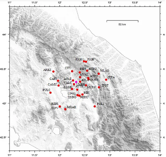
Figure 2.1: Distribution of the GPS stations used on this work. The pink dot indicates the station UMBE, placed almost at the center of the study area.

17

solutions and reference frame definition, and 3) time series analysis.

In the first step, daily GPS phase observations are used to estimate site position, adjustments to satellite orbital parameters (EOPs) and time-variable piecewise linear zenith and horizontal gradient tropospheric delay parameters by means of the GAMIT (V10.4) software [Herring et al., 2010], applying loose constraints to geodetic parameters. The ocean-loading and a pole-tide correction model FES2004 [Lyard et al., 2006], the Global Mapping Function (GMF) [Boehm et al., 2006] for both hydrostatic and non-hydrostatic components of the tropospheric delay model, the IGS absolute antenna phase center model for both satellite and ground-based antennas and the Global Pressure and Temperature (GPT) model are applied in this step. Continuous GPS (cGPS) and Survey-mode GPS networks (sGPS) are processed separately: following a simple geographic criterion, they are divided into sub-networks sharing a set of high quality IGS stations, which are used as tie-stations in the second step. Loosely constrained solutions are stored in form of ASCII GAMIT H-files and SINEX files, and contribute to the combined solution provided by Istituto Nazionale di Geofisica e Vulcanologia (INGV) [Avallone et al., 2010; Devoti et al., 2010].

In the second step the ST_FILTER program of the QOCA software [Dong et al., 2002] allows us to combine daily loosely constrained solutions with the global solutions made available by SOPAC [http://sopac.ucsd.edu] and to simultaneously realize a global reference frame by applying generalized constraints [Dong et al., 1998]. The reference frame is obtained minimizing coordinates and velocities of the IGS global core stations [http://igscb.jpl.nasa.gov], while estimating a seven-parameter transformation with respect to the IGS realization of the ITRF2008 NNR frame [Altamimi et al., 2011].

In the third step, tridimensional velocities and related uncertainties are estimated through the analysis of the position time series using the analyze_tseri program of the QOCA software. For cGPS stations, annual and semi-annual seasonal components are estimated together with a secular component while for sGPS sites only the latter component is estimated. Outliers, if present, are cleaned adopting a post-fit RMS criterion discarding values larger than 3 times the post-fit Weighted Root Mean Square (WRMS). Only stations having a minimum length of 2.5 years are retained in this analysis, as shorter intervals may result in biased estimates of linear velocities [Blewitt and Lavallee, 2002]. Residual time series contain various systematic and random errors, as well as unmodeled

18

signals; one of the major spatially correlated error sources in GPS solutions is the so-called common mode error (CME); CME can be removed from the residual time-series applying a principal component analysis (PCA) [Dong et al., 2006], improving significantly the signal to noise ratio. Velocity uncertainties are estimated adopting the maximum likelihood estimation (MLE) technique, implemented in the CATS software [Williams, 2008], considering a combination of white noise (WN) and power law noise (PL) models.

The dataset used in this work consists of 30 cGPS stations (see Figure 2.1) located within 50 km from the station UMBE, which is placed almost at the center of the investigated area. Time series for these stations are analyzed in a time span of 8 years, from 2008 to the end of 2015.

Figure 2.2 shows the occupation history of the GPS stations used in this work (the percentage of missing data is 34,6%). As described in the following chapters, reducing the amount of missing data could improve the results of an independent component analysis (ICA); for this reason stations with too shorts time series have been removed from the dataset.

The independent component analysis has been performed on raw time series, de-trended for a constant velocity term and cleaned for CME, instrumental offsets and outliers. While both raw time series cleaned for CME, instrumental offsets and outliers and

Figure 2.2: Occupation table for the dataset. Horizontal axis: time span analyzed. Vertical axis: station names.

19

raw time series cleaned for CME, instrumental offsets, outliers and for a seasonal velocity term (annual and semi-annual) have been used in the strain analysis.

2.2 Strain-rates and time-series of strain

The strain-rate field computed from geodetic velocity data measures the contribution of both seismic and aseismic deformation of the crust and is a fundamental quantity that helps in quantifying the seismic potential of active faults. Commonly, strain-rate analyses are performed starting from horizontal velocity fields, providing information on the kinematics and tectonics of a deforming region. For the study area, this analysis has been performed by Anderlini et al. [2016] showing that the area of highest deformation rate (~0.67x10-7 yr-1 of NE-SW oriented extension) is located near the crest of the Apennines; the highest compressional rate instead is located at the eastern foothills of the Northern Apennines and continues to the SE of the Adriatic coast at lower rates. The transition between the compressional and extensional regimes takes place around longitude 13°E. The Tyrrhenian sector instead exhibits relatively higher strain rates (0.3-0.4x10-7 yr-1 NE-SW oriented extension).

Alternatively, one can analyze the evolution of strain with time starting from the position time-series rather than from the stationary velocities. The cumulative strain time series, obtained from the analysis of position time series of a continuous GPS network, can be a useful tool to detect anomalous deformation signals and transients of different origin.

The strain estimation in a three-dimensional medium necessitates of the knowledge of the continuous displacement field, i.e. at each point of the medium [Pietrantonio and

Riguzzi, 2004]. Here I will describe the strain tensor and how it can be derived from

geodetic displacements and velocity measurements. Without loss of generality, for simplicity, one can consider the two-dimensional (i.e., horizontal) case [Feigl et al., 1990].

It is useful to first treat a single epoch survey, performed at time t, then the full time-dependent problem will simply follow. The calculation of the two-dimensional displacement gradient tensor from GPS data, allows the computation of the strain tensor [Allmendinger et al., 2007]:

20

(2.1)

where kui is the i horizontal component of displacement at the station k (in east and north directions), is a constant of integration, kxj is the position of the station and is the

displacement gradient tensor. Following Allmendinger et al. [2007], the equations for n stations can be rewritten as:

(2.2)

Data from at least 3 stations (n≥3) are needed because in two dimensions there are six unknowns. The solutions can be found using a least squares method. For infinitesimal strains, tensor can be additively decomposed into a strain and a rotation tensor:

(2.3)

where is the infinitesimal strain tensor and is the rotation tensor.

The diagonal elements of represent compression or dilatation according to the

sign, while the extra-diagonal ones are the shear terms. The principal deformations , are obtained by solving the classical eigenvalue problem for :

(2.4)

21

(2.5)

where and are the highest and the smallest values, respectively; the directions of the maximum shear are the orthogonal bisectors of the four angles defined by the directions of the principal deformations [Pietrantonio and Riguzzi, 2004].

A strain analysis in the investigated area has been performed through the utility

analyze_strain of the software QOCA, using as input the daily displacements in different

reference frames. The underlying assumptions of the software are:



elastic medium;



linear deformations;



2-D (horizontal) strain model.

From coordinate adjustments one can obtain the two-dimensional displacement gradient tensor for each station at each time which can be decomposed into 7 linear combinations of the displacement gradient components [Feigl et al., 1990]:

(2.6)

where u (v) is the x (y) component of displacement, , , can be used to form the strain tensor ellipsoidal, and are shear strains and is the dilatation.

Figure 2.3 shows time-series of dilatation obtained using GPS displacements as input of analyze-strain. The slope of the interpolating lines represents the dilatation rate and has the same value (~0.21x10-7 yr-1, NE-SW oriented extension) in both Figure 2.3a and 2.3b. It is coherent with the strain-rate field estimated in Anderlni et al. [2016] (see Figure 1.2b) for the region surrounding the Altotiberina fault. The latter was obtained

22

adopting spherical wavelets in order to estimate a spatially continuous velocity field from which the strain-rate field is evaluated as in Tape et al [2009].

Figure 2.3: Dilatation time series obtained using as input a) raw time series cleaned for CME, instrumental offsets and outliers, b) raw time series cleaned for CME, instrumental offsets, outliers and a seasonal velocity term (annual and semi-annual). Black dots indicate the dilatation value at each epoch with error bars (in red) obtained from the time series of the stations showed in Figure 2.1. The blue line interpolates the curve (its slope is the dilatation rate).

a

23

3. Independent Component Analysis (ICA) on

GPS time series

As discussed in Chapter 2, a way to analyze GPS time series is to model them as a superposition of functions (linear, seasonal, logarithmic, exponential, etc.) described by a proper number of parameters. Another way to perform time series analysis is to use multivariate statistics techniques such as Principal Component Analysis (PCA) and Independent Component Analysis (ICA). PCA allows to decompose time series in a certain number of components, ordered according to the amount of variance explained in the initial geodetic dataset. Similarly ICA looks for a decomposition of the original data matrix, but with some more assumptions on the source signal.

In this work the analysis of GPS time series has been performed using the ICAIM (ICA-based Inversion Method) software developed at the INGV (Istituto Nazionale di Geofisica e Vulcanologia) and University of Bologna by Adriano Gualandi [Gualandi, 2015] as an extension of the PCAIM (Principal Component Analysis-based Inversion Method) code [Kositsky and Avouac, 2010], developed at the California Institute of Technology (CalTech). After decomposing original data into the appropriate number of linear components that describe the observations, the code allows us to invert the spatial response of one or more components for slip on a predetermined fault geometry. The basic principles of ICA are exposed in this chapter as well as the fundamental steps of the ICAIM code. At last the final decomposition for stations surrounding the Altotiberina fault (ATF) is shown and discussed.

24

3.1 Independent Component Analysis (ICA): basic

principles

The Independent Component Analysis (ICA) is a multivariate statistical method searching a linear transformation of the original data that minimizes the statistical dependence between its components [Comon, 1994]. Herault and Jutten were the first to propose the problem of independent component analysis in 1983, while in 1994 Comon gave the first rigorous definition of ICA.

This technique was originally developed to deal with problems of Blind Source Separation (BSS) like the so called cocktail-party problem, describing a situation in which two people are speaking simultaneously in a room and their voices are recorded by two microphones placed in different locations. As in Hyvarinen and Oja [2000], one can express the two recorded time signals ( and ) as weighted sums of the speech signals emitted by the two speakers ( and ):

(3.1)

(3.2)

where , , , and are some parameters that depend on the distances of the

microphones from the speakers. This is a simplified model where time delays, noise and other extra factors are omitted. To solve this equation by classical methods one needs to know the parameters , otherwise it would be very difficult to find a solution. It turns

out, however, that assuming and statistically independent at each time instant allows us to separate those source signals from their mixtures and [Hyvarinen

and Oja, 2000].

A precise definition of ICA could be provided assuming the following linear statistical model [Comon, 1994, Gualandi, 2015]:

25

where X is the data matrix, A is the so called mixing matrix, S is the source signal matrix and N is some additive noise. X is an M T matrix, where M is the number of sensors and T the number of epochs; S is a L T matrix, where L is the number of sources. Independent Component Analysis is the practice of transforming these M statistically dependent sequences into L ≤ M statistically independent sequences [Choudrey, 2002].

It is useful to treat noise as one of the sources, obtaining:

(3.4)

Each M-dimensional column vector of X can be plotted as a point in the sensor space (M-dimensional) obtaining a distribution of T points. To perform an ICA means to project the sensor space onto an L-dimensional source space, described by an independent coordinate frame [Choudrey, 2002].

The underlying assumptions of the independent component analysis are:  statistical independence of the source signals;

 the values in each source signal have non-Gaussian distributions.

Technically, independence can be defined by means of the probability densities considering two scalar-valued random variables and . The marginal probability density function (pdf) of and is defined as:

(3.5)

(3.6)

where is the joint pdf of and . The two variables are said to be independent if and only if the joint pdf is factorizable as:

26

This definition extends naturally for any number n of random variables, in which case the joint density must be a product of n terms [Hyvarinen and Oja, 2000].

As regard the second assumption, that is that the independent components must be non-Gaussian for ICA to be possible, it can be shown that the joint probability density function of Gaussian variables is completely symmetric and does not contain any information on the directions of the columns of the mixing matrix A. Therefore A cannot be estimated for Gaussian variables [Hyvarinen and Oja, 2000].

Following the Central Limit Theorem, which tells that the distribution of a sum of independent random variables tends toward a Gaussian distribution, means that the observed data density is more Gaussian than the hypothetical source [Choudrey, 2002].

Hyvarinen and Oja [2000] suggest that a way to find independent variables is to measure the deviation from Gaussianity: the classical method to estimate it is kurtosis; other methods require the calculation of negentropy, mutual information (MI) or the use of generative models [Hyvarinen and Oja, 2000]. The one adopted in this work is a variational Bayesian algorithm (vbICA), developed by Choudrey [2002] and implemented in the ICAIM code (Independent Component Analysis-based Inversion Method) [Gualandi, 2015; Gualandi et al., 2016]. A short description of the basic principles of the code is given in next subsection.

3.1.1 The ICAIM software

The ICAIM code, completely written in MATLAB (The MathWorks, Inc., Natick, MA), determines the Independent Components (ICs) using a generative model and applying a variational Bayesian algorithm (vbICA) as described in Choudrey [2002]. The goal of a generative model is both to explain the observations and to match the a priori knowledge; however, this requires the estimation of different parameters, which is not always possible, and approximations, like the variational Bayesian one, are needed [Gualandi, 2015]. This approximation allows us to model each independent component i = 1,…,L by a mixture of m_i Gaussians (MoG). Each Gaussian q_i = 1,…,m_i is fully described by a mean and a precision . The vbICA algorithm imposes that these hidden

27

variables and , follow a Gaussian and a Gamma distribution, respectively. In other words, the MoG describing the i-th IC is characterized by m_i Gaussians pdf, described by

m_i normally distributed means and Gamma distributed precisions . These 2 m_i -hidden variables are thus described by some hyper-parameters that control the named distributions. In particular, the normally distributed variables are described by a mean and a precision ; while the Gamma distributed variables are described by a

scale parameter and a shape parameter . Being vbICA a generative model it is necessary to specify the a priori starting values of the hyper-parameters: in this study I specify the same a priori hyper-parameters for every IC. In particular I use , , and , , as a standard

configuration assuming that each IC is described by Gaussians as in Gualandi [2015].

The first step of an ICA is to center the data matrix X by subtracting to each time series its mean value. Then the vbICA is performed starting from a Principal Component Analysis (PCA) or a random initialization. In the first case, the starting points for the mixing matrix and for the sources are set using the U and the V values obtained through a Singular Value Decomposition (SVD) of the data matrix:

(3.8)

where the diagonal values of S are the first L singular values of X, which explain most of the variance of the data matrix, and the column of U and V are respectively the eigenvectors of the spatial covariance matrix XXT and of the temporal covariance matrix XT_{X. Such decomposition can be also obtained using the weighted low-rank}

approximation of Srebro and Jaakkola [2003], which permits to easily account for missing data and uncertainties [Kositsky and Avouac, 2010].

After having chosen the number of components that best describe the observations, as explained in 3.2.2, one could invert the spatial response of one or more components assuming a predetermined fault geometry. The inversion step will be described in details in Chapter 5.

28

3.2.2 Determining the number of useful components

In order to obtain the optimal ICA decomposition it is necessary to identify the number of components that best describe the observations, without over fitting.

The reduced χ2 test and the F-test are two commonly used procedures to get the

number of components needed to explain the dataset without reproducing the noise. These tests are based on the measure of the residuals in a L₂ norm space. A more advanced way to select the number of components for the vbICA is based on the Negative Free Energy (NFE) quantity (see Choudrey, 2002). In order to narrow down the search among several potentially good models an Automatic Relevance Determination (ARD) procedure is also introduced and combined with the NFE estimation (see Choudrey, 2002 and Gualandi, 2015).

The reduced χ2 test allows to determine the number of components such that the misfits between the original data and data reconstructed through ICA are, on average, of the order of magnitude of the measurement uncertainties [Kositsky and Avouac, 2010].

The F-test is based on the ratio of the difference between the χ2 obtained before and after adding a new component, divided by the χ2 obtained without the additional

component and multiplied by a ratio of degrees of freedom [Kositsky and Avouac, 2010]. The ARD criterion allows the determination of the number of useful components by comparing the variance value α_i (with i = 1,…,L) associated to each component; this values describe how relevant is the source for the explanation of the data. Considering a decomposition in n components, if the maximum variance is more than 10 times bigger than the smallest one, one can discard the component with the minimum variance [Gualandi, 2015; Gualandi et al., 2016].

The procedure adopted in this thesis, follows that of Choudrey [2002] and Gualandi [2015], and consists in first selecting the number of components using the ARD criterion, then testing several combinations of priors and choosing the one that minimizes the absolute value of the NFE (see also Gualandi et al., 2016).

29

3.2 ICA decomposition of GPS signals

The methods described so far have been used to analyze daily position time series of GPS stations, obtained following the procedures described in Chapter 2.

Considering that three time-series are associated to each station (one describing the motion along the East-West direction, one along the North-South and one along the vertical), the data matrix X is now a M T matrix, where M is 3 times the number of stations and T equals the number of recorded epochs.

Following Gualandi [2015], the resulting decomposition can be written as the product of three matrices (U, S, V): the sizes of U and V are M L and T L respectively, where T is the number of epochs and L is the number of independent components, while the size of S is L L. Each column of V describes the temporal evolution of one component; U, instead contains the spatial information relative to the dataset. Both U and V are non dimensional, since the unit of measurement is carried by S.

3.3 Final decomposition for the ATF

As described in section 2.1.1, the dataset used in this work consists of time series belonging to 30 cGPS stations located within 50 km from the center of the studied fault system, assumed to be in the station UMBE (Figure 2.1). The analysis is carried out on time series de-trended for a constant velocity term and cleaned for CME, instrumental offsets and outliers. The reason why time series have been de-trended before starting the ICA is that the linear signal is the most powerful signal and keeping it could cover lower signals. Furthermore, it is difficult to reproduce a linear signal with a mixing of Gaussians [Gualandi et al., 2016]. To reduce the amount of missing data, time series have been analyzed in a time span of 8 years, from 2008 to the end of 2015. The ICA has been performed using the ICAIM code, choosing a PCA initialization under the algorithm of Srebro and Jaakkola [2003] (see section 3.1.1).

30

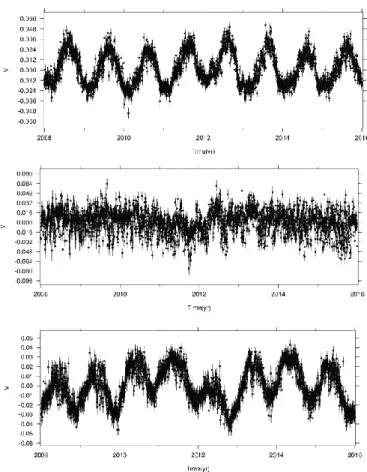
The ARD criterion suggests considering 3 components in the decomposition (Figure 3.1). Since the Signal to Noise Ratio (SNR), that is a measurement of signal strength relative to background noise, of the third component is greater than 1 only in the horizontal components I decided to analyze separately horizontal and vertical time series. In the first case, the ARD criterion indicates 4 ICs as the proper number of components, while a 3 components decomposition is suggested in the latter case. Figure 3.2 shows the ICs obtained after a separate analysis of horizontal and vertical time series, randomly changing the initialization point and choosing the decomposition with the highest NFE value among 10 random initializations.

When horizontal components are used as input for ICAIM, one more IC, showing a transient signal in 2014, appears; while using vertical time series, the third component of the original decomposition disappears.

Figure 3.2: Independent components on raw time series de-trended and cleaned for CME, instrumental offsets and outliers.

31

For this reason I decided to pursue the analysis of the ICs obtained from the horizontal time series analysis, searching for a physical interpretation of all the components.

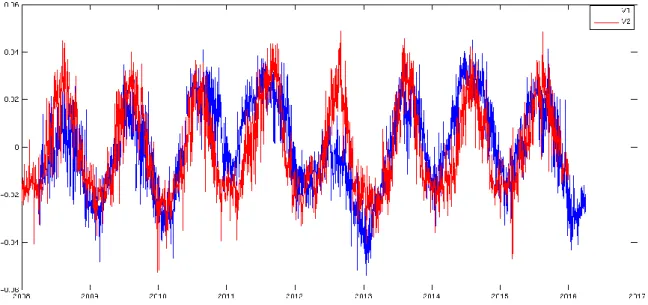
A frequency analysis on the ICs shows a dominant annual period in the first and second IC (Figure 3.3). IC1 and IC2 annual periods are out of phase of 90 days: the first component follows the second by 90 days (Figure 3.4).

IC1, IC2 and IC4 will be described in Chapter 4, where hypothesis on the interpretation of those signals will be formulated. IC3 instead seems to reproduce noise (Figure 3.2a).

The spatial response U is plotted in Figure 3.5 with vectors indicating the horizontal components and S values, which give the unit of measurement, placed on top right of each panel.

Figure 3.3: ICs obtained for horizontal (a) and vertical (b) time series.

32

IC4 exhibits a spatial response which seems to reproduce stretching, typical of normal faults. For this reason, an inversion has been performed over this component on a fault geometry placed at the center of the opening, as it will be described in Chapter 5.

Figure 3.4: Power spectral density of the ICs (IC1 (a), IC2 (b), IC3 (c), IC4 (d)) of Figure 3.2a

Figure 3.4: Superposition of IC1 (blue) shifted beyond of 90 days and IC2 (red).

b

d

c

33

Figure 3.5: Spatial response for IC1 (a), IC2 (b), IC3 (c), IC4 (d).

a

c

d

b

c

d

35

4. Analysis of the independent components

In Chapter 3 I have described how to apply ICA to GPS time series, ending up with a decomposition in four independent components, obtained using only horizontal GPS time series as input of the ICAIM code. The next step consists in finding a physical interpretation of the components, trying to identify the sources of those signals.

In this chapter I will analyze each IC of the final decomposition, except for the third one which seems to reproduce mainly noise. Some correlations with other signals will be presented, which could explain the presence of those deformation signals (or fingerprints) in GPS records.

4.1 First component

As seen in Chapter 3, the first IC of the final decomposition exhibits a seasonal periodicity. Figure 4.1 shows that in a region around 2011-2013, the temporal component of IC1 (black) differs from a sinusoidal curve (red). This is the most powerful signal in the decomposition, being the Signal to Noise Ratio (SNR) for this component bigger than 1 for more than of the stations. The time series of the station GUB2 (Figure 4.2) is reported as an example of a time series in which the IC1 signal presence is clear at visual inspection.

36

In section 4.1.1 the correlation between the first component of the IC decomposition and the cumulative precipitations is described.

Figure 4.1: First independent component of the final decomposition (black). A sinusoid with annual period (red) has been superimposed to the IC1 in order to show that the IC1 signal differs from a sinusoid in the time interval 2011-2013.

Figure 4.2: Horizontal components of the time series of station GUB2. Blue dots indicate surface displacement at each epoch, while the red curve is the reconstruction based on the ICA.

37

4.1.1 Correlation with rainfall

In order to analyze the precipitation trend, rainfall values are taken from repositories of the European Commission's 6th Framework Programme (EU-FP6) project ENSEMBLES (http://ensembles-eu.metoffice.com). They are high resolution daily gridded data obtained through a three-step process of interpolation of precipitation data, recorded by meteorological stations located all around Europe [Haylock et al., 2008]. The catalog contains the millimeters of rainfall per day for each cell of a regular 0.25° 0.25° grid.

In order to obtain the daily amount of rainfall (mm/day) in the same region analyzed with the ICAIM software (within 50 km from the station UMBE) and in the same time span (2008-2015), a stacking has been performed over each cell of the grid belonging to the analyzed region. After that, curves of cumulated precipitation, obtained varying the number of accumulation days, have been compared with the temporal component of the first IC finding that a 190-days accumulation curve best fits the IC1 trend, with a

Figure 4.3: Superposition of the first IC (blue) and of the 190-days rainfall accumulation curve (red). Both curves have been rescaled.

38

correlation of 0.6. The precipitation curve has been centered along the y axis and both curves have been rescaled in order to be compared. Figure 4.3 shows the 190-days rainfall accumulation curve (red) superimposed on the temporal component of the first IC (blue). It can be seen that the precipitation curve departs from a sinusoidal behavior in 2012; indeed, that year was characterized by a very slow rainfall rate that seems to have influenced the horizontal component of surface displacement in the region of interest. The departure from a sinusoidal signal is partially present also in the vertical component decomposition (Figure 3.2b), but the first IC of that analysis is out of phase with respect to the cumulated rainfall. Indeed it has the same phase of the IC2 resulting from the analysis of the horizontal time series that is described in next section. This mixture of signals may be caused by the higher level of noise in the vertical component, typical of GPS measurements.

This analysis suggests that seasonal geodetic displacements seem to reflect a lithospheric response to the seasonal variation of hydrological surface loads. The hydrological cycle in fact, has been shown to be capable of producing measurable deformations of the lithosphere [e.g. Christiansen et al., 2007; Bettinelli et al., 2008]. Modeling of these effects requires knowledge of the hydrological properties of the crust and is beyond the scope of this thesis.

4.2 Second component

As seen in Chapter 3 (Figure 3.2a), the second IC of the final decomposition describes a sinusoidal signal with annual period (Figure 4.4). The analysis of the local seismic catalog shows an annual variation of the number of earthquakes that correlates with this IC, as detailed in the following of this section.

39

4.2.1 Correlation with the seismic catalog

I have analyzed the seismic catalog of the study region in order to search for an annual periodicity in the seismicity rate. This analysis has been performed on the Italian Seismological Instrumental and parametric Data-basE (ISIDE) catalog of INGV (iside.rm.ingv.it), selecting events occurred in the same region analyzed with ICAIM (within 50 km from the station UMBE) and in the same time span (2008-2015), as well as on events of another catalog of relocated seismicity (Luisa Valoroso, pers. comm.) which covers a time span of almost 4 years (April 2010 – May 2014). Histograms (green) indicating the number of events per day for each catalog are reported in Figure 4.5.

Next section contains a description of the Schuster spectrum code used to search periodicities in the seismic catalogs of the ATF area.

40

Figure 4.5: Events for the ISIDE catalog (a) and for the catalog of relocated seismicity (b). The green histograms represent the number of events per day. The continuous lines indicate the cumulative number of earthquakes with magnitudes above the detection thresholds (M_l = 1.2 in panel a and M_l = 1 in panel b) of the original catalog (blue line) and of the de-clustered catalog (red line).

a

41 4.2.1.1 Schuster spectrum software

The Schuster spectrum software was developed by Thomas J. Ader and Jean-Philippe Avouac [Ader and Avouac, 2013] as a generalization of the Schuster test [Schuster, 1897]. While the Schuster test allows to determine whether a given periodicity is present or not in a seismic catalog, the Schuster Spectrum looks for periodicities in a given period range allowing finding more than one periodicity, if present.

The Schuster test is a statistical test that associates a phase to each event of the seismic catalog:

(4.1)

where is the time of event number k and T is the tested period. The phase of each event is represented in the complex plane as:

_(4.2)

Starting at the center of the complex plane, after K events the total distance from the origin will be:

_(4.3) where:

(4.4)

(4.5) and where:

(4.6)

42

(4.7)

Calling D the final distance obtained when K equals the total number of events in the catalog, Schuster [1897] defines the probability (Schuster p-value) that a distance equal to or greater than D can be reached by a random walk as:

(4.8)

where N is the number of events in the catalog. Therefore, 1-p represents the significance level to reject the hypothesis that earthquakes occur randomly. This means that a lower p-value corresponds to a higher probability to have a periodicity at the period T in the catalog.

It can be seen [Ader and Avouac, 2013] that the logarithm of the Schuster p-value is independent of the tested period T, depending only on the number N of events in the catalog and on the amplitude α of the seismicity rate variations:

(4.9)

Ader and Avouac [2013] generalize the Schuster test to overcome its main problem: while it is sure that a periodicity in the catalog gives a low p-value, a low p-value itself cannot indicate unambiguously a periodicity in the catalog. Calculating a spectrum of Schuster p-values allows to resolve this issue and to search for any unknown periodicities, as explained hereafter.

In order to determine the subset of periods to test suitable to obtain a complete spectrum of Schuster p-values for the catalog, it is important to notice that when testing a period T, the catalog gets stacked over that period, so the continuous range of periodicities around T that remain coherent throughout the stacking process gets tested. For this reason the first step is to define a proper period sampling in order to avoid both long computation time due to oversampled testing and skipping to test any relevant period. Two consecutive tested periods have to verify the condition:

43

(4.10)

where is the period increment, is the i-th tested period, t is the length of the time series and ε determines the period sampling. The optimal value of ε is ε₀ ≈ 1 (see Ader and Avouac [2012] for the proof).

The second step is to determine the probability threshold below which a Schuster p-value can be regarded as indicating with confidence a periodicity of the catalog. Following Ader and Avouac [2012] the expected value of the maximum Schuster probability for a given tested period is:

(4.11)

which means that the expected value is higher for higher periods.

If a p-value is significantly lower than the threshold value, the probability to have a periodicity in the catalog is high. In other words a low p-value means that the null hypothesis that earthquakes take place randomly is rejected.

The Schuster spectrum code needs as input the epochs of the events in the catalog and a range of periods to be tested. The proper range should be between _{and ,}

where is the length of the catalog [Ader and Avouac, 2012].

Sometimes declustering the catalog is necessary because keeping events not related to the background activity (e.g. aftershocks or swarms) might conceal some periodic variations in the background seismicity rate [Ader and Avouac, 2012]. This misinterpretation of clusters is due to the stacking process and it results in low p-values for periods above a given period. Since a not properly declustered catalog shows a cloud of low p-values at large periods, performing a Schuster spectrum would help to understand whether in a catalog a given periodicity is real or an artifact produced by the presence of clusters, while a simple Schuster’s test cannot achieve this target.

44 4.2.1.2 Results

A first test to search periodicities has been performed on the ISIDE catalog in the range between 8 10-4 _{and 8 years. 11768 events, with magnitudes above M}

l = 1.2, have

been analyzed. I have estimated the magnitude detection threshold from the magnitude-frequency distribution of earthquakes. Results are shown in Figure 4.6, where Schuster p-values are plotted as a function of the period tested, in a log-log graph (note the reverse scale in the y-axis). A periodicity of one year is evident but the cloud of points, with low p-values (periods larger than 10-2 yr) suggests the presence of clusters in the catalog. Therefore, a declustering seems to be necessary in order to verify if the low p-value obtained at 1 year describes a real periodicity of the catalog. I have performed the declustering using the Reasenberg algorithm [Reasenberg, 1985], implemented in the ZMAP software [Wiemer, 2001], using default parameters. The code looks for temporally and spatially dependent events in the catalog (aftershocks occurring after some foreshock) and removes them returning a catalog composed of independent events. Reasenberg [1985] defines an interaction zone as a spatiotemporal window and assumes that if an earthquake occurs within the interaction zone of a previous event it is classified as an aftershock and thus it is removed from the catalog.

After the declustering, only 3473 independent events remain in the catalog. The cumulative number of earthquakes before and after the declustering process is plotted in Figure 4.5a (red and blue lines respectively). Figure 4.7a, instead shows the Schuster spectrum for the declustered catalog. The periodicity at one year seems to disappear in this case, while low p-values at large periods indicate that some clusters are still present in the catalog.

The analysis of the relocated seismicity gives different results. A first test on the catalog reveals the presence of clusters, that have to be removed. In this case declustering reduces the number of events from 5005 to 1098 events. The cumulative number of earthquakes before and after the declustering process is plotted in Figure 4.5b (red and blue lines respectively). Figure 4.7b, instead shows the Schuster spectrum for this catalog. The declustering process seems to be well fulfilled, since no low p-values are present at high periods except for that at 1 year. This means that an annual periodicity for this catalog is

45

highly probable. This analysis results in extremely low probability (less than 1%) that seasonality in this catalog is due to chance.

The reason why the analysis of the two catalogs produces different results could be the imprecise location of hypocenters in the ISIDE catalog that might affect the results of the declustering. It could be that earthquakes occurring closely in space are instead localized at a distance greater than the selected interaction zone and thus they are considered as independent. Indeed the percentage of residual events after the declustering is 30% for the ISIDE catalog, while for the catalog of relocated seismicity it is 22%. Figure 4.8 shows epicenters location for both declustered catalogs.

Figure 4.6: Schuster spectrum for the ISIDE catalog. Grey dots indicate the probability values corresponding to each of the period tested. The black dashed line in the bottom identifies the 99% confidence level (0.01 x ). Dots among this level are darker. The dashed blue line indicates the

46

Figure 4.7: Schuster spectrum for the ISIDE catalog (a) and for the catalog of relocated seismicity (b) both declustered. Black dashed lines in the bottom identify the expected value and the 95% and 99% confidence levels, while the dashed blue line indicates the 1year period. Only the catalog of relocated seismicity shows a periodicity at 1 year.

a

47

Another way to represent the results consists in plotting the 2D walk of the phase angle and verify if the probability that a random walk reaches the distance D is sufficiently low. To do this it is useful to first translate the time series so that it starts from time . The 2D walk (red curve) described by the phases is shown in Figure 4.9 for the period T=1 yr. Since the red curve ends out of the circle of 99% confidence level one can conclude that the probability to have an annual periodicity in the catalog of relocated seismicity exceed the 99%.

Figure 4.10 shows a stacking of the number of earthquakes per week for the catalog of relocated seismicity with superimposed a sinusoidal curve (red) with annual period. The same red curve has been superimposed on the plot of the second independent component of the ICA switched in sign (Figure 4.11) in order to visualize the correlation between the two

Figure 4.9: 2D walk of the phase angle , with K=1,…,N (N red dots), calculated for the period of 1 year, represented in the complex plane. The x component of each point of the curve is

, while the y component is . Green, pink and blue circles represent the 80%, 95% and 99% confidence levels, respectively.

Figure 4.8: Epicenters location of the background events of the ISIDE (red dots) and the relocated (blue dots) catalogs.

48

signals. This correlation can be seen also in Figure 4.12 where a stacking of seismicity and of the IC2 over 1 year are superimposed. Figure 4.13 shows a curve (red) of daily mean temperature of the area superimposed on the temporal component of the second IC (blue). Temperature data have been downloaded from the dataset of the ENSEMBLE project (http://ensembles-eu.metoffice.com) and processed as described in section 4.1.1 for precipitation data, then daily mean temperature has been centered around y = 0 and rescaled. The correlation between the two signals of Figure 4.13 is 0.82. Therefore, considering the anticorrelation between the temporal component of the IC2 and seismicity (Figures 4.11 and 4.12), it turns out that the highest earthquakes rates are observed during winter, when temperature is lower, while the lowest earthquakes rates take place during summer months, when temperature is higher. In other words, temperature variations seem to modulate earthquakes occurrence in this area. Therefore seismicity seems not to be modulated by hydrological cycle as it is proposed for Nepal by Bettinelli et al. [2007], since the IC1, that correlates with rainfall and the IC2, that correlates with seismic periodicity are out of phase of 90 days.

Figure 4.9: 2D walk of the phase angle , with K=1,…,N (N red dots), calculated for the period of 1 year, represented in the complex plane. The x component of each point of the curve is

, while the y component is . Green, pink and blue circles represent the 80%, 95% and 99% confidence levels, respectively.

49

As described in Chapter 1, seismicity in this region is mostly due to microearthquakes (M_L<3.0) occurring at high rate. Many studies [e.g. Gao et al., 2000; van

Dam et al., 2001; Ebel and Ben-Zion, 2014] have demonstrated that microearthquakes

Figure 4.10: Number of earthquakes per week (blue bars) of the catalog of relocated seismicity. A sinusoid with annual period has been superimposed to the histogram in order to emphasize the annual periodicity of seismicity.

Figure 4.11: Temporal component of the IC2 (blue) switched in sign and sinusoidal curve of seismicity of figure 4.9 (red). This indicates an anticorrelation between the seismic activity and the geodetic displacement associated to the second IC.

50

Figure 4.12: Superposition of a stacking of the number of earthquakes per week over 1 year (yellow bars) and of a stacking of the IC2 over 1 year switched in sign and translated along the y axis in order to have only positive values. Both the histogram and the black curve are rescaled.

Figure 4.13:Mean temperature curve (red) superimposed on the temporal component of the second IC (blue). Temperature values have been centered along the y axis and rescaled.