Turbulence and structures in the solar wind

(1)

pour obtenir le titre de

Docteur en Sciences

de l’UNIVERSITE de Nice-Sophia Antipolis

Dottore di ricerca in Fisica Applicata

dell’UNIVERSITA di Pisa

Discipline: Astronomie et Astrophysique

présentée et soutenue par Luca MARRADI

Turbulence et structures dans le vent solaire

Thèse dirigée par Thierry PASSOT et Francesco Califano

soutenue le 28 Novembre 2011

Jury:

M. G. Belmont Directeur de recherche Rapporteur

M. L. Sorriso-Valvo Chercheur CNR Rapporteur

M. F. Pegoraro Professeur Examinateur

Mme. H. Politano Directeur de recherche Examinateur

M. D. Del Sarto Maitre de conférences Examinateur

M. F. Califano Professeur Co-Directeur de Thèse

(2)

(3)

in the direction perpendicular to the ambient magnetic field. These problems were studied by means of one-dimensional numerical simulations with two different methods: a FLR-Landau fluid (FLR-LF) model that extends anisotropic magnetohydrodynamics by retaining low-frequency kinetic effects such as Landau damping and finite Larmor radius corrections, and a hybrid Vlasov code in 1D-3V phase space dimensions (HV). Preliminary investigations were performed in the context of compressible Hall-MHD that demon-strated a possible Alfvén wave cascade in the parallel direction at scales smaller than the ion inertial length. Simulations of the FLR-LF model in quasi-perpendicular directions with a random forcing aiming at mim-icking the tail of the Alfvén cascade show a non-resonant ion perpendicular heating and the development of the mirror instability which constrains the system to remain near instability threshold. The FLR-LF model has then been extended to include the effect of a weak amount of collisions described by a BGK operator. Simulations including collisions show a very good agreement with satellite data. We also performed simula-tions with the HV code where a forcing on the electric field code was introduced. These simulasimula-tions showed the generation of a power-law spectrum with slope -5/3 at scales larger than the ion skin depth, and slope -7/3 in the short-wavelengths range, together with the formation of “perpendicular shocks” and magnetic

holes.

Résumé

Deux aspects de la turbulence dans le vent solaire à des échelles de l’ordre du rayon de Larmor des ions ont été abordés: le chauffage anisotrope du plasma et les propriétés spectrales de la cascade turbulente dans la direction perpendiculaire au champ magnétique ambiant. Ces problèmes ont été étudiés au moyen de simulations numériques unidimensionnelles utilisant soit un modèle dit “FLR-Landau fluid” (FLR-LF) qui étend la magnétohydrodynamique anisotrope en retenant les effets cinétiques basse fréquence (effet Landau et corrections de rayon de Larmor fini), soit un code Vlasov hybride 1D-3V dans l’espace des phases (HV). Des études préliminaires menées dans le contexte de la MHD-Hall compressible, ont démontré qu’une cascade d’ondes d’Alfvén est possible dans la direction parallèle, à des échelles plus petites que la longueur inertielle des ions. Des simulations du modèle FLR-LF dans une direction quasi-perpendiculaire avec un forçage aléatoire modélisant la cascade Alfvénique ont mis en évidence un chauffage perpendiculaire non-résonnant et le développement de l’instabilité miroir qui contraint le système à rester au voisinage du seuil. Les simulations de ce modèle, incluant l’effet de faibles collisions (décrites par un opérateur de BGK) montrent un très bon accord avec les données des satellites. La simulation HV, avec un forçage sur le champ életrique a permis de révéler la formation d’un spectre en loi de puissance en -5/3 aux échelles plus grandes que la longueur inertielle des ions et en -7/3 aux échelles plus petites, ainsi que la formation de chocs perpendiculaires et de trous magnétiques.

(4)

iii

Riassunto

Questa tesi si focalizza sullo studio della dinamica turbolenta del vento solare. In particolare mi sono occupato d’indagare i principali fenomeni scaturiti quando una tale dinamica inizia a coinvolgere scale paragonabili al raggio di Larmor. Gli argomenti discussi nella tesi riguardano: il riscaldamento anisotropo del plasma, e le proprietà degli spettri elettromagnetici relativi alla cascata turbolenta nella direzione perpen-diculare al campo magnetico ambiente. Questi problemi sono affrontati utilizzando due differenti metodi: il primo, chiamato FLR-LF, permette di includere nei modelli magnetoidrodinamici sia l’effetto cinetico del Landau damping sia l’effetto dispersivo giocato dalle correzioni del tensore di pressione dovute alla finitezza del raggio di Larmor (FLR); il secondo riguarda invece l’utilizzo di un codice Vlasov ibrido, rispettivamente unidimensionale nello spazio delle posizioni e tridimensionale nelle spazio delle velocità (HV). Studi pre-liminari, eseguiti per mezzo del modello Hall-MHD comprimibile, hanno dimostrato la possibilità di una cascata di onde di Alfvén lungo la direzione parallela al campo magnetico ambiente capace di raggiungere scale più piccole della lunghezza inerziale ionica. Ulteriori simulazioni numeriche del modello FLR-LF in direzione quasi-perpendicolare con l’aggiunta di un forzaggio “random” atto ad imitare la coda della cas-cata Alfvénica, mettono in evidenza un riscaldamento non-risonante sulla specie ionica lungo la direzione perpendicolare al campo magnetico ambiente, favorendo lo sviluppo di instabilità “mirror”. Quest’ultima vincola il “range” di valori sia dell’anisotropia di temperatura ionica sia del beta ionico. Una estensione del modello FLR-LF è stata inoltre realizzata includendo, attraverso un operatore BGK, l’effetto delle col-lisioni. Simulazioni numeriche che tengono conto delle collisioni mostrano un ottimo accordo con i dati forniti dai satelliti. Infine, simulazioni col codice HV, all’interno del quale un forzaggio sul campo elet-trico viene applicato, hanno prodotto sia spettri eletromagnetici con pendenze di -5/3 e -7/3 rispettivamente su scale maggiori e minori della lunghezza inerziale ionica sia strutture elettromagnetiche quali “shock” perpendicolari e buchi magnetici.

(5)

(6)

v

Preface

In this thesis I studied two of the hottest topics related to the turbulent dynamics of the solar wind plasma:

1. the break of the magnetic spectrum; 2. the temperature anisotropy;

First of all, the interest for studying the electric and magnetic spectra is motivated by the necessity to understand how the energy, injected at a scales larger than the ion skin depth (di), cascades down to the

electron scales and then dissipates. Actually, the turbulent heating of plasma could explain the observed radial temperature profile of the solar wind protons at 1 AU. The term “break of the magnetic spectrum” derives from the abrupt slope change that takes place around the proton-cyclotron frequencies fcp. These

observations show that the Kolmogorv power law (f−5/3_{), developed for frequencies below} _f

cp (inertial

range), is replaced by another power lawf−2.5for frequencies above the proton-cyclotron. Even though the exact mechanism which leads to the break of the magnetic spectrum is still under debate [1, 2] its origin seems to be the dispersion and not the dissipation as believed in the past [3]. At the moment, data provided by Cluster spacecrafts [4, 5] have pointed out that the Kinetic Alfvén wave (KAW) [6, 7] is the most probable responsible mechanism for the second cascade. In fig. (1) we show the power spectrum of the interplanetary magnetic field (IMF) fluctuations at 1 AU versus frequency, reported by the Wind spacecraft. A clear break in the interplanetary magnetic field fluctuations that takes place close toΩp = 0.096Hz (proton-cyclotron

frequency).

Moreover, satellite data show that electromagnetic (e.m.) energy is mainly channeled along the direction perpendicular to the ambient magnetic field.

Motivated by the:

1. importance that kinetic effects play around the proton-cyclotron frequency; 2. dominance of the perpendicular e.m. energy compared with the parallel one;

detailed numerical investigations on the solar wind dynamics at typical kinetic scales, resulting from a turbulent cascade along the direction strictly perpendicular to the ambient magnetic field, have been per-formed by using a kinetic code (hybrid Vlasov). In order to trigger the e.m. cascade, I implemented a forcing

(11)

Figure 1: The power spectrum of the interplanetary magnetic field (IMF) fluctuations at 1 AU versus

fre-quency. Measurements were provided by the Wind spacecraft. [7].

in the Hybrid-Vlasov code (see chapter 9) and applied it on the electric field components perpendicular to the direction of integration. This last condition (_{∇ · E = 0) allows to preserve the charge neutrality} assump-tion of the Hybrid-Vlasov code. I applied the forcing on the largest scales of the system so that the kinetic scales evolve because of the turbulent cascade and not of the particular analytical form of the forcing. I used four decades in wavenumber space to separate the forcing from the kinetic scales. The main results that I obtained are:

• in agreement with the GS95 theory I obtained an e.m. power scaling law with slope _{−5/3 in the} wavenumber rangekdi < 1 while a −7/3 slope for the small wavenumber range kdi > 1. Even

though the physics underlying the development of the turbulence is different, it should be noted that this last result is surprisingly in agreement to the gyro-kinetic simulations performed by Howes et al. [8];

• a perpendicular collisionless shock is formed in a self-consistent way during the development of the turbulent cascade. In order to exclude the possibility of a numerical shock, I verified that the Rankine-Hugoniot conditions for a fast-magnetosonic shock are satisfied. Furthermore, contour plots of the velocity proton distribution function (vdf), averaged along the vz direction and taken close to the

shock ramp, have shown the presence of ions rotating around the z axis;

• couplings between the ion Bernstein waves (IBW) and the magneto-sonic mode take place along the cascade.

• magnetic holes are formed as well in a self-consistent way because of the turbulent cascade. It should be noted that these structures are not in pressure balance.

The second research issue, temperature anisotropy, comes from the observed satellite data. These data show that:

• the perpendicular proton temperature decreases slower than what is expected from a double-adiabatic approximation;

(12)

TABLE DES MATIÉRES 3

Figure 2: The picture shows the evolution of proton temperature anisotropy in the solar wind from 0.3

AU to 1 AU provided by Helios observations. The contour plots are referred to the observed frequency of beta_k,p, T⊥,p/Tk,pat 0.3 AU (dashed) and 1 AU (solid), respectively. Dash-dotted and dotted line represent

the temperature anisotropy as a function of theβ_k,p. [9].

In particular, it is interesting to focus the attention on Fig. (2) where the solar wind evolution (from 0.3 AU to 1 AU) of the observed frequency of proton temperature anisotropy (T⊥,p/Tk,p) and proton

parallel beta (β_k,p) is displayed as a function of the heliocentric distance. The radial evolution of the (βk,p, T⊥,p/Tk,p) is represented by the dash-dotted line and the double-adiabatic prediction is represented by

the dotted line. The different slope between the dash-dotted line and the dotted one suggests that some kind of heating mechanisms, as for instance the ion-cyclotron resonance or the dissipation of the electromagnetic turbulent cascade, are at work when the solar wind expands from 0.3 AU to 1 AU.

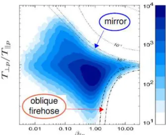
Recently, Hellinger et al. [10] have pointed out that the distribution bins of the relative frequencies of (β_k,p, T⊥,p/Tk,p), provided by WIND for the slow solar wind, seem to be constrained by oblique instabilities.

Looking at contour plot of fig. (3), where the frequencies of (β_k,p, T⊥,p/Tk,p) are reported, it appears

surprising that such data do not extend beyond the contour of a near-zero maximum growth rate for the above mirror and the oblique firehose instabilities. These last observations are in contradiction with the predictions of the linear theory, according to which proton-cyclotron and parallel firehose would dominate for all but largeβ_k,p.

I investigated the competition between the heating mechanisms and the mirror instability that takes place along the upper border of fig. (3). In order to approach the above mentioned problem I used the Landau fluid code (see chapter 1) that extends the anisotropic magnetohydrodynamics model including linear Landau damping and finite Larmor radius corrections (FLR). These effects are supposed to play an important role in the competition between the plasma turbulent heating and mirror instability. First of all, I considered the purely collisionless system and I used a white noise forcing in time applied on the velocity field in order to develop Alfvénic turbulence. A non-resonant ion heating along the perpendicular temperature and the development of the mirror instability, that constrains the system to remain near instability threshold, are the first important result in my numerical simulations. However, when the numerical frequencies of (T⊥,p/Tk,p,

β_k,p) are compared with the mirror frontier, represented by the dotted black line, a slight discrepancy is observed.

(13)

Figure 3: A logarithmic color scale is shown in the picture. The maximum growth rate (in units of

proton-cyclotron frequency) in the corresponding bi-Maxwellian plasma for the mirror instability (dotted curves) and the oblique fire hose (dash-dotted curves) are over plotted on the contour. [10].

In agreement with slow solar wind data provided by WIND, I introduced the physics of collisions (isotropization, thermalization effect of the temperature) in the Landau fluid model by using a Bhatnagar-Gross-Krook (BGK) operator (see chapter 2).

I chose a BGK collision operator because it:

• represents the simplest class of collisional operators; • is easy to implement in the Landau-fluid model.

In such a physical condition the effect of collisions improves the agreement between the numerical and the observed contour plots. This result suggests that deviations from bi-Maxwellianity are quite small in the slow solar wind regions, explored by the WIND spacecraft.

Thanks to the results reported in my thesis it is now possible by using the same physical parameters to:

• extend one dimension Landau fluid simulations into a three-dimensional geometry in order to take into account the competition between the parallel and perpendicular turbulent cascade;

• explore the 2D-3V Vlasov simulations with the ambient magnetic field strictly perpendicular to the direction of integrations x, y. In this way it will be possible to verify turbulent cascade origin of the collisonless shock and magnetic holes structures.

Moreover, preliminary works have been performed on comparing the 1D FLR-LF and the hybrid Vlasov, in which a forcing has been implemented on the magnetic field component perpendicular with respect to the ambient magnetic field. Actually, technical problems due to the correct implementation in the Hybrid-Vlasov code of the white noise in time forcing , do not allow the quantitative comparison between the two codes. Anyway, qualitative results are reported in the conclusions of this thesis.

(14)

5

Chapter 1

Introduction

One of the most suitable environments for the in situ study of a fully developed turbulence state is the solar wind (SW) plasma [11]. This SW state is represented by a flux of particles, flowing out from the solar corona holes. The SW is composed by 95% of protons and electrons (in roughly equal numbers)

with a remaining small portion of alpha particles and isotopes that are streaming along the solar open lines of the magnetic field. The physical properties of the solar wind depend on the space region taken into account. In order to give an idea about the order of magnitude of the physical parameters as density of the particles, mean velocity along the ambient magnetic field and magnetic strength, the average values are: n _{∼ 5 cm}−3, V _{∼ 450 km/s and |B| ∼ 10 nT. For a long time spacecraft measurements have been} able to detect a wide range of frequencies (10−2 Hz up to 102 Hz) and the corresponding scales length extrapolated by the Taylor’s hypothesis [12] of the fluctuating fields into the solar wind. However, from these spacecraft measurements the dynamics of this ”low” collisional plasma still continuous to be hard to understand because of the multitude of the typical time and spatial scales driven by collective Coulomb interactions between protons and electrons. This variety of scales observed in the SW points out one of the principal features of plasmas, the so-called multi-scale nature. By using the analysis presented in [13] it is possible to summarize the spatial scale (1/k) range as follows:

• Mean free path:

1. k_kλmfpi ≫ 1 collisonless regime where the wave-particle interaction plays a determinant role;

2. k_kλmfpi ≪ 1 collisional regime; with λmf pithe mean free path of the ion species;

• Ion scales:

1. atk⊥di≪ 1 ions and electrons are magnetized and the magnetic field is frozen into the ion flow;

2. atk⊥ρi∼ 1 the energy exchange via wave-particle interaction can heat the ions;

3. atk⊥di≫ 1 the electrons and ions are magnetized and unmagnetized, respectively;

withρi= Vth,i/Ωcithe ion gyro-radius,di= VA/Ωcithe ion skin depth andVth,i, VAthe ion thermal

and the Alfvén velocity, respectively; • Electron scales:

(15)

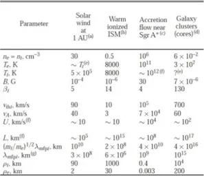
Figure 1.1: Typical plasma parameters of different space environments are shown.

2. atk⊥ρe∼ 1 the electrons begin to suffer the wave-particle interaction;

3. atk⊥de≫ 1 the electrons and the ions are unmagnetized;

withρe = Vth,e/Ωce the electron gyro-radius, de = VA/Ωce the electron skin depth andVth,e the

electron thermal velocity;

and for the time scales

• Ion cyclotron:

1. at_{ω ≪ Ω}ci (ω the frequency of the e.m. fluctuation) there are no-resonances between ion

parti-cles and e.m. fields;

2. at_{ω ≫ Ω}cithere are resonances between ion particles and e.m. fields;

• Electron cyclotron:

1. at_{ω ≪ Ω}ce no-resonances between electron particles and e.m. fields are at play; atω ≫ Ωce

resonances between ion particles and e.m. fields take place;

In Fig. (1.1) the typical orders of magnitude of the plasma parameters of four different astrophysical environments are listed: SW, interstellar medium (ISM), accretion flows and Galaxy clusters.

When a specific phenomenon has to be studied, the wide range of typical scales involved in the plasma dynamics represents in general a serious problem. In particular, the dominant phenomena, in each range between these characteristic scales are different and demand different modelling, while, the electromagnetic (e.m.) nonlinear interactions, that take place along the different parts of frequency spectrum, connect a large range of physical scales and frequencies making possible several energy transfer scenarios from the driving (outer scale) to dissipative scales of the system. The explanation of the magnetic and electric spectra still represents one of the formidable issue in magnetized plasma space turbulence. The rapid development of

(16)

1.1. CASCADE PICTURE 7

Figure 1.2: The picture ([14]) shows the Richardson energy cascade. In the top big whorls, synonymous of

large structures, have evolved in the little whorls until a complete destruction takes place.

computers and the new space cluster missions have made possible to approach systematically the plasma turbulence problem. Numerical simulations and spacecraft analysis feedbacks are today the best approach to verify or deny the different turbulence theories.

1.1 Cascade picture

In the literature, turbulence is frequently associated with the word ”cascade”. The choice of this term takes origin from the idea developed in 1922 by Richardson and it illustrated in Fig. (1.2). According to this theory the transfer of energy from large to small scales is realized through non-linear mechanisms that led fictitious structures, defined by Richardson as eddies, to a progressive fragmentation. The continuous decaying process breakdown when the typical dimension of the eddy approaches the viscosity scale. A typical laminar (i.e. without efficient scale mixing) fluid dynamic turbulence example, that everyone can experience in order to verify the Richardson idea, is the mixing by a spoon of milk and coffee in a cup. What happens is that the two liquids will be perfectly mixed. Looking at the phenomenon from a hydrodynamic point of view, the mixing can not be directly produced by the spoon because its dimension is much larger than the microscopic particles of milk and coffee. Therefore, the large scale energy injected into the system by the spoon motion will generate velocity fluctuations on smaller and smaller scales. This process will stop when the typical dissipative scales of the system will be approached. As a matter of fact, if the same experiment described above is repeated but with a cappuccino, the cream of the milk present in the cup will slow down the mixing. In fact, it is possible to observe the formation of intricate coffee spirals due to the cream presence. It may be argued that the energy transfer to small scales inferred by the shaking action of the spoon is reduced by the resisting structures created by the cream. The physical picture of the cascade followed by viscosity dissipation, can be formalized mathematically through the following one-dimensional

Burger’s equation for the hydrodynamics velocityu(x, t):

∂u ∂t + u ∂u ∂x = ν ∂2_u ∂x2. (1.1)

(17)

• the mean of the solutionu is zero.

It should be noted that the last condition can be always achieved by solving the Burger’s equation for the velocity fluctuation, defined as: δu(x, t) = u(x, t) − hu(t)i, where:

hu(t)i = _2π1 Z 2π

0

u(x, t)dx.

Under these conditionsu(x, t) can be expressed as:

u(x, t) =

+∞

X

k=1

Ak(t)sin(kx).

By using the above expansion foru(x, t) in Eq. (1.1) and taking into account the relations:

∂u ∂t = +∞ X k=1 ˙ Ak(t)sin(kx). ∂u ∂x = +∞ X k=1 kAk(t)cos(kx) ν∂ 2_u ∂x2 = −ν +∞ X k=1 k2Ak(t)sin(kx) u∂u ∂x = − +∞ X m=1 +∞ X l=1 Am(t)Al(t)sin(lx)cos(mx)

the Burger’s equation in the Fourier space reads:

+∞ X k=1 ˙ Aksin(kx) + +∞ X l=1 +∞ X m=1 mAlAmm 2 (sin(l + m)x + sin(l − m)x) = −ν +∞ X k=1 Akk2sin(kx) (1.2)

(18)

1.1. CASCADE PICTURE 9

Z 2π 0

dxsin(px)sin(qx) = πδpq

Eq. (1.2) is reduced to the:

˙ Ak+ +∞ X m=1 m AmAk−m 2 + AmAk+m 2 ! = −νk2Ak k = 1, 2, · · · , +∞. (1.3)

when the LHS and RHS are multiplied bysin(kx) and integrated between 0 and 2π. It seems clear that the

role of the viscosity term is to damp the amplitude of the k-mode. When neglecting the terms in bracket, a new differential equation is obtained:

˙

Ak= −νk2Ak=⇒ Ak(0)e−νk

2_t

showing explicitly the damp effect of the viscous term. Conversely, the presence of the nonlinear terms in Eq. (1.3) acts in order to transfer the momentum Akassociated with the scale k to the component k −

m, k + m. In order to illustrate this process, let us consider the sum of Eq. (1.3) restricted only to the first

three modes (m=1,2,3). By taking into account thatAp = 0 if p ≤ 0 or p > 3 the following equations are

obtained: ˙ A1+ A1A2 2 + A2A3 = −νA1. ˙ A2+ A1A1 2 + A1A3 2 = −4νA2. ˙ A3+ 3A1A2 2 = −9νA3. (1.4)

If as initial condition A1(0) 6= 0 is taken then ˙A2(0) 6= 0 because of the presence of the nonlinear

termA1A1/2 in the equation for A2. Similarly, if A2 6= 0 then ˙A3 6= 0 yielding a A3 6= 0. This chain

of excitations will be stopped when the momentum, the quantity transferred along the cascade, will reach the viscosity scale. This simple example illustrates how the nonlinear interactions are able to transfer and spread the momentum into a wide range of scales. The continuous energy cascade, towards small scale in plasmas, is of particular interest when the energy reaches the kinetic scale lengths giving rise to a multi-scale evolution. Finally, it should be noted that in the example reported above I have used a coherent phase approximation in theu(x, t) field unlike the usual random phase one (see Ref. [15]) used in turbulence.

(19)

is actually a vortex structure generated in a turbulent fluid motion and identified by its scale lengthl, velocity u and a turnover time tl = l/u. From an experimental point of view, eddies can be generated when a fluid

flux streams through a grate with a mesh size of dimension L. In particular, an eddy will be created in

the downstream region of the grate when the Reynolds number, defined as Re(L) = uL/ν (with u typical

mean hydrodynamic velocity, andν the dissipation), takes sufficiently large values. It should be noted that Re represents a ”measure” of the ratio between the nonlinear and the viscous term in the Navier-Stokes

equation [14]:

Re(l) ≃ u · ∇u/(ν∇2u_{) ≃} ul

ν (1.5)

The important finding achieved by Kolmogorov was that in highly turbulent systems (_{Re ∼ 10}3 _{− 10}6) the energy injected into the system through the so-called outer scaleL, is transferred at a constant rate ǫ to

small dissipative scales lν across a range of scales (lν ≪ l ≪ L), defined as the inertial spectrum. In the

inertial range the physics is “universal”, i.e. independent of the specific energy injection and dissipation mechanisms. A brief summary of the hypothesis at the base of the K41 ideas are listed below following the guidelines given by Schekochihin et al. in Ref. [6]. The K41 theory is based on four assumptions concerning the nature of the inertial range:

1. homogeneity (no special points); 2. scale invariance (no special scales); 3. isotropy (no special directions); 4. local interactions between scales.

Starting from these assumptions, it is possible to get some important relations betweenǫ, defined as the

energy transfer rate per unit mass and unit time between vortices, and the typical spatial and velocity scale corresponding to eddies of different ”size”. The idea of Kolmogorov theory is that the energy injected on the larger eddies (outer scale) is transferred by means of local interactions from intermediate vortex to smaller and smaller ones up to the dissipative scalesld≃ ν/ud, whereudis the typical velocity corresponding told.

The dissipative scale is determined by the conditionRe(ld) ≃ 1. Kolmogorov postulated that in stationary

conditions ǫ should be constant and expressed as a combination of the only quantities characterizing the

vortices, the velocityuland the scalel:

ǫ ∼ u

3 l

l (1.6)

(20)

1.2. FROMKOLMOGORV TOGS95 11 ǫ ∼ u 3 d ld ld ∼ ν3 ǫ !1/4 ud∼ (νǫ)1/4.

whereudis the characteristic velocity at the dissipative scaleldand we used the condition Re(l = ld) = 1.

By using the previous relations it is easy to link the larger scales of the inertial range, identified by eddies with typical spatial scaleL and velocity V, with the dissipative ones by the following formulas:

L ld ∼ Re 3/4 V ud ∼ Re 1/4_.

The Kolmogorov wavenumber scaling of -5/3 of the kinetic energy spectrumE(k) comes out from the

following considerations:

• in stationary condition each eddy receives from the bigger ones, per unit time cascade timetland unit

mass, a continuous and constant amount of kinetic energyǫ;

• the energy received from each vortex is entirely transmitted to the smaller ones;

Taking into account the previous considerations the kinetic energy associated with the scale l (in the

inertial spectrum) isTl≃ u2_l. By using the relation:

T(k) ≃ Z 1/ld

k=1/l

E(k′)dk′,

withE(k) the spectral density of the kinetic energy, and by takingdT(k)

dk , it follows:

E(k) ∼ Cǫ2/3k−5/3

withC depending on the energy injection rate.

The first work, aimed at extending the K41 theory to incompressible hydromagnetic plasmas, appeared in 1965 in a Kraichnan’s manuscript [17] (KR65). Before discussing the scaling energy law of the KR65,

(21)

frequencies, the basic fluctuations are represented by the Alfvén waves propagating along the magnetic field lines. Kraichnan argued that rewriting the MHD equations in Elsasser variables z±_{= u ± b/}√4πρ in the

following way: (Ref. [18]):

∂ ∂t + z ∓ · ∇ ! z±_{∓ v}A∇kz± = −∇p + ν + η 2 ! ∇2z±+ ν − η 2 ! ∇2z∓ ∇ · z∓ = 0 (1.7)

nonlinear interactions could take place only between counter-propagating fluctuations. In the previous equation: ρ is the fluid density, u the hydrodynamics velocity, p the pressure, b the magnetic field, B0

the background magnetic field, vA = B0/√4πρ the Alfvén velocity, η the resistivity, ∇k the gradient

takes along the B0 direction. The advantage to cast the MHD equations in a more symmetric form given

by Elsasser equations is that their incompressible solutions assume a simple form. Putting z+ = 0 (or z−= 0) the nonlinear terms disappear and taking into account that in the inertial range the contribute of the

dissipative terms in RHS of Eq. (1.7) is negligible, we can deduce the following equations:

∂ ∂t + vA∇k ! z−_{= −∇p +} ✟✟✟✟ ✟✟✟✟ ✯0 ν + η 2 ! ∇2z±+ ✟✟✟✟ ✟✟✟✟ ✯0 ν − η 2 ! ∇2z∓ ∇ · z∓= 0. (1.8)

By taking the projection of the first equation in the perpendicular plane with respect to the k direc-tion, we get that z− _{= f (x − v}At) is a generic fluctuation propagating along the ambient magnetic field

at the Alfvén velocity. Similarly, the case with z+ leads to the following solution f(x + vAt)

propagat-ing along the B0 at the Alfvén velocity but in the opposite direction z−. The existence of Alfvénic-like

fluctuations (δz−_{, δz}+_{) counter-propagating along B}

0, suggested to Kraichnan that non-linear interactions

betweenδz−, δz+allowed to develop an energy cascade (Alfvénic turbulence). Starting from the same K41 assumption of local interaction between fluctuations of comparable scale and assuming for fluctuations of typical spatial scale l that δz+_l _{∼ δz}−_l _{∼ δu}l ∼ δbl, Kraichnan summarized the wave-wave interaction as

follows:

1. an Alfvénic timeτAis taken by one wave to pass through the other;

2. during the interaction time a velocity amplitude variation takes place in both the interacting fluctua-tions. The order of the variation is: ∆δul∼ δul

τA

τl

!

(22)

1.2. FROMKOLMOGORV TOGS95 13

3. a weak interaction conditionδul≪ ul, τA≪ τlis assumed.

The weak interaction condition formulated by Kraichnan allows not only to order the Alfvén and the nonlinear time, but it makes possible to define a cascade time tcas. In particular tcas is defined as the

time required to changeδul by an amount comparable to itself. The previous condition is mathematically

obtained by the relation: ∆δul∼ δul. If the changes in amplitude accumulate as a random walk

t X ∆δul∼ δul τA τl t τA !1/2 (1.9)

takingt = tcas and imposing t

X

∆δul ∼ δul, it follows in Eq. (1.9) thattcas ∼ τ_l2/τA∼ l2vA/lku2l. The

knowledge of thetcasandδulallowed Kraichnan to make the same steps as Kolmogorov, illustrated in the

previous equations. Substitutingtcasin Eq. (1.6) he got:

δul∼ (ǫvA)1/4l−1/4_k l1/2⇒ E(k) ∼ (ǫvA)1/2k−3/2. (1.10)

It is worth noticing that KR65 theory assumes isotropy in the spatial scale, i.e.l_k_{/l ∼ l in Eq. (1.10). The}

KR65 was considered as a valid turbulence theory until Matthaeus et al. [19] showed, thanks to spacecraft observations, the anisotropic nature in the SW of the e.m. fluctuations. Thus the fluctuations spatial scale isotropy assumption adopted in K41 and KR65 had to be reconsidered. The first theoretical attempts to explain the observed anisotropy came from a re-examination of the Alfvén-wave turbulence in MHD. Basically from KR65 the assumptions claimed that the turbulence can be regarded as a resonance process involving a three Alfvén waves scattering process characterized by the following conservation relations:

k1+ k2 = k3⇒ kk,1+ kk,2= kk,3

ω±(k1) + ω∓(k2) = ω±(k3) ⇒ kk,1− kk,2 = kk,3

(1.11)

where each wave is identified by its own wavevector k and frequencyω±(k) = ±kkvA. From Eq. (1.11), it

is immediate to point out that:

1. turbulence cascade is mediated by waves withk_k = 0;

2. there is no parallel cascade;

3. anisotropy between parallel and perpendicular spatial scales is formed.

In 1997 Goldreich and Siddhar [20] showed that even taking into account in the KR65 the anisotropy between the parallel and perpendicular directions, there is no way to extend the KR65 model in order to reproduce the in-situ observations of e.m. fluctuations. In order to understand the last point we are going to reconsider the KR65 theory in which the isotropy condition is replaced by spatial scale anisotropy. In

(23)

1 ≫ τ_τA l ∼ ǫ1/4 (k_k,0vA)3/4l1/2_⊥ ⇔ l⊥≫ lGS = ǫ1/2 (kk,0vA)3/2 ∼ δu2 L v2 A 1 k2 k,0L . (1.12)

Therefore to ensure the weak interaction condition for all scales of the inertial range,lGSscale must not

belong to the inertial range. However, looking at the expression oflGS, we observe that:

• lGSremains fixed when the outer scales are fixed;

• lν ∼ LR−3/4e ,lη ∼ LR−3/4m (whereη, ν are respectively the diffusivity and viscosity) depend on the

magnetic and viscous Reynolds number (Rm= δuLL/η, Re= δuLL/ν), with L the outer scale;

• the dissipative scaleslν, lη still represent the end of the inertial range.

Taking into account that:

lν lGS ∼ R −3/4 e vA δuL !2 k2_k,0L2, lη lGS ∼ R −3/4 m v2 A δu2 L ! k2_k,0L2

it appears clear that forRe, Rmnumbers sufficiently high we get the following ratios:

lν

lGS ≪ 1,

lη

lGS ≪ 1.

In such a way the weak interaction condition (Eq. (1.12)) will not be verified for all the inertial scales. This fact pushed Goldreich and Siddhar to the conjecture that at thelGSscale the system turns into a new

regime called strong turbulence in which the following relation is satisfied:

τA∼ τl⇔ l_k vA ∼ l⊥ δul (1.13)

In particular, the idea behind Eq. (1.13) is that as energy flows down to small scales, the equilibrium betweenτA∼ τlis forced by the system itself. The balance condition among these times allows to remove

the ambiguity previously encountered. By setting the time cascadeτl= l⊥/δulassociated to the scale

fluc-tuationl⊥and by repeating the same K41 steps, an energy spectrum asE(k⊥) ∝ k−5/3_⊥ for the perpendicular

fluctuation scales is obtained. In conclusion, the different theoretical frames for describing turbulence can be summarized as follows:

(24)

1.3. SOLAR WIND 15

1. weak turbulence theory, satisfied by the conditionτl≫ τA, consists in considering only the resonant

nonlinear interactions, (see Eq. (1.11)) which are the most efficient for small amplitudes, and which draw an e.m. cascade purely perpendicular with respect to the ambient magnetic field;

2. the strong turbulence (τl ≪ τA) theory considers the non-resonant interactions, less efficient, but

concerning an e.m. cascade even if along the direction parallel to the ambient magnetic field;

3. the critical balance that represents an extension of the weak turbulence theory toward the boundary

τl= τA, where the cascade is not strictly perpendicular (kk= k2/3⊥ ).

1.3 Solar wind

The aim of this section and the following one is to introduce the context and the problem considered in this thesis.

1.3.1 Fast and slow wind

One of the main difficulties of astrophysical plasmas comes from the impossibility to experimentally reproduce in the laboratory the extreme low collisionality conditions corresponding to high Reynolds num-bers of space plasmas (_{∼ 10}10). However, both the SW and the EMS (Earth magnetosheath) represent a very favorable magnetized plasma turbulent environment in which a large set of data can be provided by

in-situ spacecraft measurements. These measurements give valuable feedback on turbulent models. In order

to solve the open question about the heating processes at play in space environment as intercluster medium (ICM), interstellar medium (ISM), and solar corona, a detailed understanding of the following phenomena occurring in SW and EMS driven by turbulence: anisotropy magnetic energy cascade and evolution of the temperature anisotropy in the SW. The starting point of this study is the investigation of the turbulence pro-prieties in the SW. As discussed in the introduction of this Chapter, the SW is a mixing of charged particles composed principally by protons and electrons. The SW, roughly speaking, is divided into two main parts: the fast (FSW) and the slow solar wind (SSW) characterized, as shown in Table (1.3), by different physical parameters, a different mean velocity and particle density.

The distinction between SSW and FSW emerges basically from three important differences pointed out by spacecraft measurements:

• different origin on the sun;

• heliocentric evolution of the e.m. fluctuations;

• presence of macro-structures convected by the SW itself.

The FSW is identified by a mean velocityvfsw≃ 700Km/s and is originated in the polar solar regions,

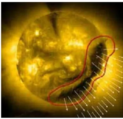
as shown in Fig. (1.4). It is pushed out in the interplanetary space through the so-called coronal holes, open magnetic lines anchored on the solar corona. On the contrary, the SSW is characterized by a lower mean velocityvssw ≃ 400Km/s and it is originated from the equatorial regions which can be observed in the solar

(25)

Figure 1.3: The tables reported in the picture compare typical parameters of the fast and slow SW at 1 AU. The tables are taken from [21].

Figure 1.4: The picture (http://c2h2.ifa.hawaii.edu/Pages/Education/sun_wind. php) shows the Helmet streamer. SSW flows in the interplanetary space along the flank of this coronal structure.

atmosphere during the solar eclipse. During the solar minimum, the polar coronal holes are considerably widened, such that they can reach the equatorial regions. As a consequence of this expansion, interactions between FSW and SSW can take place and form the so-called stream interface located in front of the fast stream where strong compressive phenomena can take place. Fig. (1.7) shows measurements in proton density, proton temperature and module of the magnetic field provided by STEREO at 1 AU around a stream interface.

1.3.2 Solar wind and turbulence

First evidence on the SW as turbulence medium was reported by Coleman et al. [22] in 1968. By using the data provided by the spacecraft MARINER 2, Coleman et al. studied the statistics of the interplanetary fluctuations relative to the period August 27 - October 31, 1962. The interesting conclusion reached was that the magnetic energy, showed in Fig. (1.8) in a log-log plot, is distributed over an extraordinary wide frequency range, varying from one cycle per solar rotation (roughly 28 days) up to10−1_{Hz with a power}

(26)

1.3. SOLAR WIND 17

Figure 1.5: A sketch (taken from [])of the magnetic field structures observed in the solar corona.

Figure 1.6: The picture (http://c2h2.ifa.hawaii.edu/Pages/Education/sun_wind. php) shows the Helmet streamer. SSW flows in the interplanetary space along the flank of this coronal structure.

frequency ranges, based on the data reported from three different spacecraft, MARINER 2, MARINER 4,

OGO-5, was given by Russell et al. in the famous paper [23]. The following scaling in the frequency range

was reported:

• f−1up to10−4Hz.

• f−3/2between the intermediate frequencies10−4 _{≤ f ≤ 10}−1Hz.

• f−2up to 1Hz, in the high-frequencies range.

The Fig. (1.9) shows the plot of the magnetic energy spectrum obtained by Russell. Fifty years later the first

Russell’s classification, the observations performed by Alexandrova et al. [25] and Saharaoui et al. [4], have

shown a clear separation of the SW frequency spectrum in three distinct ranges:

• the energy injection region (outer scales) considered as the source of the turbulent cascade and iden-tified by frequencies below10−4_{Hz with a frequency spectrum slope given by ∼ f}−1_{, where} _{f is the}

(27)

Figure 1.7: The picture is provided by the paper of Simunac et al. [24] and shows a streamer interface at

around 1AU. The gray windows separate the FSW (on the left side) from the SSW (on the right side). From the top to the bottom are represented, respectively: bulk solar wind speed, proton density, thermal proton speed.

(28)

1.3. SOLAR WIND 19

Figure 1.9: The magnetic power spectra as a function of frequency is showed in the picture. This figure is

taken from the Russell’s paper [23].

• the inertial region located in the frequency range_{∼ 10}−4Hz to 10−1_{Hz is characterized by a scaling}

in the magnetic energy spectrum intermediate between the Kraichnan and Kolmogorov (f−1.62); • the dissipative range characterized by a power lawf−α _with_{2 < α < 4 that takes place above the}

ion-gyro frequency Ωci ∼ 1Hz. The role of this region on the final transformation of the magnetic

energy to thermal energy is still not well understood.

Recently, technological progresses have allowed to observe the cascade of the turbulent e.m. fluctuations up to electron frequency (_{∼ 40 Hz). Using data provided by CLUSTER, Sahraoui et al. have plotted (see} Fig. (1.10)), for frequencies into the range [10−3_{Hz − 100Hz], the magnetic energy in parallel (black and}

green lines) and perpendicular (red and blue lines) direction to the ambient magnetic field, as a function of frequency. They observed that, before reaching the electron frequencies (_{∼ 1 Hz to 40 Hz), the turbulent} e.m. fluctuations undergo a second cascade with a frequency power lawf−2.50. Sahraoui et al. have shown that the:

• kinetic theory of the kinetic Alfvén wave (KAW) turbulence allows to explain the observed second cascade;

• when the KAW cascade approaches the electron gyroscale the effect of the collisionless electron Landau damping on the KAW allows to justify the dissipation observed from satellite measurements.

(29)

Figure 1.10: The picture represents a log-log plot of the magnetic spectrum along 5 frequency decades. The

parallel (black) and perpendicular (red) magnetic spectra correspond to the FGM data (f < 33Hz). The green and blue lines are the parallel and perpendicular magnetic field plotted by STAFF-SC data (1.5 < f < 225Hz). Dashed and dotted lines are respectively the noise level of the STAFF-SC measured in the laboratory and in-flight. The straight black lines are power law fits to the spectra. The arrows indicate characteristic frequencies, fcp, fρp, fλp, fρe, fλe, corresponding to the proton cyclotron, the proton Larmor,

the ion skin depth, the electron Larmor and the electron skin depth, respectively. This figure is taken from the Sahraoui’s paper [4]

1.3.3 The role of the expansion in the solar wind

In addition to the still unsolved problems present in the SW of the energy dissipation and the anisotropy fluctuations, in situ measurement of the SW particle distribution function (d.f.) have shown clear signatures of non-Maxwellian shape. In a natural way, the SW expansion leads to strong temperature anisotropy. This last point can be illustrated, at lower order, through a simple double-adiabatic (or CGL) fluid model. Assuming that:

1. SW is expanding spherically with a velocity vSW constant and directed along the radial direction (in

the Sun rest frame);

2. magnetic field B is directed along the radial direction and its magnitude varies with radial distanceR

such thatB = B0(R0/R).

and taking into account that two adiabatic invariantsT⊥/B, (TkB2)/n2 are conserved in the CGL model, it

is possible to conclude that the temperatures will scale with distance as:

T⊥∝ R−2 and Tk = const.

where theT⊥, Tkare the perpendicular and parallel temperatures with respect to the ambient magnetic field,

respectively. The previous relation allows to calculate βp ∝ (nTk,p/B2) ∝ Tk,p/T⊥,p ∝ R2. As shown

by Matteini et al. [9], a direct comparison between the analytical and experimental radial evolution of the (βp, Tp,⊥/Tp,k), measured by Helios spacecraft in the fast wind at 0.3 AU and 1 AU (see fig. (3) in

(30)

1.3. SOLAR WIND 21

Ref. [9]), points out a discrepancy between the experimental anti-correlation ofβp andTp,⊥/Tp,k, and the

CGL prediction. This evidence shows that some heating mechanisms are at play along the perpendicular direction in the heliocentric range 0.3-1AU. An interesting problem connected with the proton temperature anisotropy observations has been recently pointed out by Hellinger et al. [10]. They have performed a statistical analysis on large slow SW dataset of the Wind/SWE data (from 1995-2001) relative to the proton temperature anisotropyTp,⊥/Tp,kand proton betaβp,k. They compared the possible role played by

proton-cyclotron, mirror, parallel and oblique firehose instabilities, on the distribution of (Tp,⊥/Tp,k, βp,k) values.

In particular, the authors calculate the threshold of these instabilities starting from the linearized system of Vlasov-Maxwell equations, in which Maxwellian and bi-Maxwellian d.f. are assumed for the electron and proton species, respectively. They find that for β_p,k _{≥ 10 the observed proton anisotropy temperature is}

constrained by oblique firehose and mirror instability (see Fig. (1) in Ref. [10]). It is worth noticing that results of the linear theory, in plasmas withβ_p,k _{≥ 10, favor instabilities as proton cyclotron instability}

and the parallel firehose instead of the oblique firehose and mirror instability. The possible sources of disagreement between observation and linear theory are summarized by Hellinger et al. [26] in the following points:

• presence of non-negligible abundance of alpha particles, and other plasma parameters as electron temperatures;

(31)

Figure 1.11: Observations performed by Helios, Pioneer Venus, Ulysses and Cassini from 0.34 to 8.9 AU of

mirror mode waves. The snapshot is taken from [27].

On the other hand, as it is shown in Chapter (5), the FLR-Landau fluid code has been able to reproduce the slow solar wind WIND/SWE dataset in the (βp, Tp,⊥/Tp,k) diagram close to the mirror instability

thresh-old. Moreover, the introduction of a small amount of collisions in the FLR-Landau fluid model improves the quality of the fit.

1.3.4 Magnetic holes

The SW is characterized by the presence of magnetic field structures so-called magnetic holes (MHs), which are defined as magnetic field depressions whose duration can vary from one to a few hundred seconds. Fig. (1.11) shows MHs observation provided by the spacecraft Helios, Pioneer Venus, Ulysses and Cassini. Where exactly MHs are generated is still unclear. Russell et al. [27] have suggested that MHs are signatures emerging from the development of mirror instability created closer to the Sun and convected by the SW over long distances, in plasma regions stable with respect to the mirror instability. However, it should be noted that mirror modes are observed also in other space-plasma environments: the Earth’s magnetosheathh, the Saturn’s magnetosheathh, the helio-sheath. The properties that characterize the mirror modes are:

• a shape corresponding to a magnetic depression (dip or hole) or a magnetic enhancement (peak or hump);

• a phase velocityvφ,mirror≃ 0 in the plasma reference frame;

(32)

1.4. ASHORT STATE OF ART OF THESWPLASMA TURBULENCE. 23

• spatial magnetic field variations take place in highly oblique directions (quasi-transverse);

• magnetic field fluctuations mostly affect the parallel component, defined with respect to the direction of the ambient field (linearly polarized);

Recently, a statistical study of a mirror structure varying the plasma parametersβkand the ion anisotropy

ratioT⊥/Tk, has been carried out by Soucek et al. [28]. They found that the feature of mirror structures

depends on the local plasma state with respect to the mirror instability threshold. Peaks are frequently observed in unstable plasma regions for mirror, while in agreement with the observations by Stevens and

Kasper [29] at 1AU in the SW, dips appear in stable regions. These last observations led Winterhalter et al. [30] to confirm the scenario supposed by Russell et al. in which MHs are remanants of mirror mode

instability convected by the SW. At the same time, hybrid numerical simulations performed by Buti et

al. [31] have shown that MHs can be formed when large-amplitude right-hand polarized Alfvénic wave

packets propagate at large angles with respect to the ambient magnetic field.

In agreement with the Russell et al. assumptions, the study of MHs can be used to extract important pieces of information about plasma conditions in regions close to the Sun. Moreover, a conspicuous interest in studying these structures is also given by the feedback that MHs have on the global dynamics of the SW plasma. Finally, an interesting and recent result reported in Chapter 6, shows that by performing 1D-3V hybrid Vlasov simulations magnetic holes are formed as result of a perpendicular cascade, triggered by an external driver applied to the plasma at large wavelengths.

1.4 A short state of art of the SW plasma turbulence.

In this section, we will focus on the problem of modes channeling beyond the inertial range and the breaking of the magnetic spectrum at the ion Larmor radius ρi. An important point, still debated in the

scientific community, concerns the identification of the main kinetic mechanism that pushes the SW plasma to develop a clear break in the magnetic energy spectrum around the proton-gyrofrequency. In the past, spacecraft technological limits did not allow to provide any informations beyond the first breaking point of the magnetic energy located around the proton-cyclotron frequency. This fact led to a splitting of the scientific community in two parts. The first one [32, 33] supports the idea that the changing in the slope is due to a dissipative effect played by the ion cyclotron resonance (IC); the second one [34, 35] claims the presence of a new energy cascade.

Fig. (1.12) indicates the separation of the magnetic spectrum in three distinct range: inertial, dispersive and dissipative. Over the years the idea of a second cascade beyond the breaking point became more and more convincing. Since 2005, Bale et al. [5] using 195 min of data during the interval 00:07:00-03:21:51 on 19 February 2002 provided by Cluster mission reached the conclusion that, after the breaking point located in the spectrum aroundkρi ∼ 1, a potential second cascade formed by kinetic Alfvén waves (KAW) was

activated. In panel (b) of Fig. (1.13) they reported an estimation of the phase velocity (vφ) obtained by

using the Faraday’s law. In particular, the ratio among the y and z component of the electric and magnetic fields (Ey/Bz), with y, z referred to a GSE coordinate system (http://sspg1.bnsc.rl.ac.uk/

SEG/Coordinates/geo_sys.htm) is plotted. They showed that vφ displays a change of slope at

scaleskρi∼ 1. They found that the KAW velocity phase relation [6] is in a very good agreement with the

(33)

Figure 1.12: The picture, extracted from the paper [35], points out the slope variation along the cascade in

the wavenumber space of the magnetic spectrum. In particular: at large scale the Kolmogorov cascade is associated to the inertial range followed by the so called dispersive intermediate range dissipative range

from an observational point of view by Sahraoui et al. [36] and numerically by Howes et al. [37] using a gyrokinetic (GK) approach. For the first time, the detailed work developed on SW data performed by

Sahraoui et al. [36] gives evidence of a second breaking point located around the Doppler-shifted electron

gyro-radius scale corresponding to a frequency _{f ∼ 35Hz in the magnetic spectrum plotted in Fig. (1.10).} Starting from these observations and in order to investigate the possible role played in this scenario by the KAW, Saharaoui et al. have performed a numerical linear analysis on the Vlasov-Maxwell (VM) equations by using the same SW data discussed in the mentioned paper. They found, as reported in Fig. (5) of Ref. ([36]), that KAW can propagate obliquely along a wide range of scales before being damped at electron gyro-scale (kρe) where the linear damping rate over the real part of the frequency becameγ/ωr∼ 1.

Recently, numerical gyrokinetic results obtained by Howes et al. [8] by means of AstroGK code [38], have confirmed and reinforced the hypothesis of a KAW cascade behind the first breaking point k⊥ρi ∼ 1. In

particular, Howes et al. show a magnetic power spectrum scaling ofk−2.8which is in quantitative agreement with the in situ spacecraft measurements of the solar wind dissipation range.

In Fig. (1.14) the perpendicular energy of the electric (red) and magnetic (blue) fields are plotted as function of thek⊥ρi along the inertial range. In agreement with the GS95 theory, a Kolmogorov scaling

(k−5/3_⊥ ) appears clear, whereas beyond the breaking point electric and magnetic spectra show a flattening (k−1/3_⊥ ) and a steepening (k−7/3_⊥ ) power laws respectively. It should be noted that the gyrokinetic equations, integrated in the code, are obtained taking gyro-average of the V-M equation [39]. This procedure, even if retains the Landau damping effect and a full description of the FLR terms, does not allow to describe cyclotron resonances and trapping effects. The physical justification of this fact advanced by Howes et

al. concerns the critical balance idea of the GS95. The key point stressed by them is that when the turbulence

generates scale such that k⊥ρi ∼ 1, the parallel scale will be of order of magnitude given by kk ∝ k2/3⊥

leading to Alfvén frequencyω = k_kvA≪ Ωci.

In conclusion the role of the linear Landau damping in the nonlinear situation described above does not underestimate the dissipative effects that take place on the e.m. fluctuations. Even if the KAW cascade seems to be strongly supported by observations, new insight based on an extension of the KR65 theory to homogeneous whistler turbulence was elaborated by Naritia et al. [40]. Recently, Podesta et al. [41] have developed an heuristic model in which, for plasma parameters typical of high-speed SW at 1 AU, the KAW

(34)

1.5. COLLISIONLESS SHOCK 25

Figure 1.13: In the top, the wavelet (upper) and the FFT (lower) of theEy(green) andBz(black) spectra are

reported as function of the wavenumberkρi. The electric spectra are multiplied by factors in order to stay

above the magnetic spectra. Kolmogorov spectrum is well developed over the intervalkρi ∈ (0.015, 0.45).

A first and a second breaking point are respectively formed in both fields when the scalekρi≈ 0.45 before

andkρi ≈ 2.5 are reached. In the bottom, the ratio between Ey/Bzis estimated in the plasma frame. The

figure is taken from [5].

cascade is dissipated before reaching the electron gyroscale (k⊥ρe∼ 1).

This fact supports the idea that the power spectra, observed around the electron gyroscales, must be developed by other wave modes. Following this new idea, Gary et al. [2] have performed numerical two di-mensional Particle-In-Cell (PIC) simulations of magnetized, homogeneous, collisionless electron ion plasma showing, as reported in Fig. (1.15) the existence of a forward whistler cascade on the scales ranging between

0.1 < k⊥ρe< 1 and 0.1 < kkρe< 1.

1.5 Collisionless shock

A short introduction on collisionless shocks will be presented in this section. The attention will be focused on the perpendicular and quasi-perpendicular collisionless shocks in order to develop an useful theoretical framework for interpreting the numerical simulation results illustrated in the Chapter 6.

From MHD shock to ion reflection

The first observations carried out by the spacecraft MARINER and IMP of CS encouraged the develop-ment of theoretical models able to interpret such structures. The first was to pay attention on the macro-scale

(35)

Figure 1.14: The figures taken from [37], are the result of a gyrokinetic simulation performed by AstroGK

code [38] using βi = 1., Ti/Te= 1. and a box size L⊥ = Lz = 20πρias parameters. In the bottom, the

magnetic (solid line) and electric (dashed line) energy spectra (see their definition in the mentioned paper) are plotted as function of thek⊥ρiin the MHD regime (0.1 < k⊥ρi < 1.). In the top, the energy spectra for

δB⊥(solid line),δBk (dash-dotted line) and the perpendicular electric energy associated withE⊥(dashed

line) are plotted as function of thek⊥ρialong a spectral range0.5 < k⊥ρi < 10.

of the CS, postponing in such a way the study of shock ramp region ∆sh. This can be understood by the

following reasons:

1. basic mechanisms of CSs formation had to be understood before studying the CS in a microscopical framework;

2. the typical scale of∆shless than or of the order ofρciimply the presence of kinetic effects in the shock

ramp. Therefore the Vlasov-Maxwell equations have to be solved in order to investigate properly the ramp.

The first approach that allowed to shed light on the CS formation mechanisms was the assumption of the macro-scale point of view. The latter allows to assimilate the complex spatial structures of the CS to a perfect discontinuity between the upstream and downstream regions. In this framework the MHD appeared to be the proper model to attack the CSs formation problem. The scientific community realized that within a MHD framework, three kinds of shocks were possible: fast, slow and intermediate Alfvén. Those kinds of CSs can be formed only when the flow velocity is able to exceed the corresponding wave phase speed associated with the fast, slow or intermediate wave. When this condition is realized, a steepening process takes place due to nonlinear evolution of a dispersive wave disturbance that leads to generate in the system smaller and smaller scales.

The competitive role of dispersion and dissipation/anomalous dissipation effects in shock formation represented the guidelines for more than one decade of theoretical efforts. An important step forward in the CS investigations came out in the theoretical work due to Marshall [42]. In that paper Marshall et

(36)

Figure 1.15: The color contours, taken from the paper [2], represent the logarithmic evolution of the

mag-netic field fluctuations energy at three different times reported in electron cyclotron unit (Ωe) as function of

thek_kdeandk⊥de(wherek⊥ = ky). The red spot reported atΩet = 0 represents the initial distribution

of the whistler modes. It should be noted that the anisotropy developed is consistent with the perpendicular propagation of whistler turbulence predicted by [1].

al. showed that for a CS with the magnetic field perpendicular to the normal of the shock front, there was

a critical Mach number, Mcrit ∼ 2.6, above which the anomalous dissipation was insufficient to sustain

the shock front propagation in the plasma. It was necessary to find out a new process in order to provide the proper ”dissipation”. A very important contribution in this research was given by Sagdeev [43]. The idea concerned the reduction of the incoming flux of particles by a counter-streaming beam in the upstream region generated, by a partial reflection of the incoming flux. However, in order to validate the theory and to obtain a more detailed description of this mechanism, it was necessary to wait for the technological progress of the spacecraft and the computers.

Figure 1.16: The picture represented the transition between the quasi-perpendicular and the quasi-parallel

shock due to the curved Bow shock structure coming out from the interaction between the SW and the geomagnetically field. The figure was taken in the paper [44].

(37)

• the different regions of the bow shock constituted by quasi-perpendicular and quasi-parallel region as shown in Fig. (1.16);

• the foreshock, defined as the region upstream from the Earth’s bow shock that is magnetically con-nected to the bow shock and contains charge particles coming from the bow shock and both solar wind plasmas;

• the individuation of the foot (see Ref. [45]) in the bow shock along the quasi-perpendicular region. An important point confirming the theoretical investigation was the first evidence from the spacecraft of the reflected ions in the Earth’s bow shock, reported by Montgomery et al. in Ref. [46]. The satellite observations also confirmed the slowing down of the mean SW normal velocity after the shock to sub-"fast magnetosonic" one. The agreement between the foot structure observations reported in Ref. [45] and the theoretical predictions based on specular reflection model of the ions from the shock ramp, allowed to point out the existence in the foreshock region of a free energy source able to trigger drift instabilities generated by relative motions among the incoming ion flux of the SW and the reflected ion beam [47]. Spacecraft observations of the foreshock region allowed to find a broad spectra of low frequency e.m. modes propagating in all directions with and against the solar wind. In particular, it was observed that some of these lowest frequency fluctuations could steepen, generating in the solar wind large amplitude low frequency or quasi-stationary structures so-called wave packets. These last appeared as spatially localized and traveling magnetic ramps or shocklets, the origin of which is still not well understood. Furthermore, data provided by satellite ISEE2 in the bow-shock showed, as can be seen in Fig. (1) of Ref. [48], a tendency of the electron d.f. to become gradually flat when the satellite crosses the shock ramp. This fact led Feldman et al. [48] to point out the importance due to the presence of field-aligned electron beams and the possibility to develop electrostatic instability as the ion-acoustic and the Buneman instability. However, in the following paper [] a complete review of the present problems in Earth’s bow shock are illustrated and it will be given more in details.

Numerical simulations

The increasing computer resources have given a significant contribution to the progress in the CS physics. The great advantage of the simulations was represented by the possibility to overcome the intrinsic limita-tions of satellite measurements, following therefore in details the evolution of different physical regimes by changing the plasma parameters as βi, βe, MA, Te/Ti. Numerical simulations also give the possibility of

investigating closer the electric and magnetic structures generated by the system as well as the dynamics driven by the presence of electron and/or ion temperature anisotropy. The first numerical investigations on the magneto-sonic shocks were performed in the seventies by Biskamp [49, 50]. In particular the authors addressed the study of the plasma heating and the reflection of particles during the shock formation pro-cess. First hybrid simulations, in which the ions are considered as particles while the electrons are taken as a massless isothermal and neutralizing fluid, permitted to explore the microscopic mechanisms in sub-critical perpendicular shocks and the competitive role between the steepening and the dissipative/dispersive

(38)

processes. However, the main outcome of the numerical investigations performed in the eighties, was the confirmation that ion reflection and foot formation in front of super-critical and perpendicular shocks took place. A careful exploration of different CS geometries, defined by the angle formed between the upstream magnetic field and the normal to the shock, allowed to establish a quantitative threshold between the sub-and the super-critical CSs. At present, the attention in numerical CS simulations is focused on problems concerning the temporal variations of the shock front, new mechanism of shock reformation [51] and elec-tron heating mechanism at play in high Mach number perpendicular shocks. A complete overview of the mentioned problem can be found in [52].

1.5.1 Typical scales in collisionless shocks

The interaction among a super-magnetosonic flow with an astrophysical obstacle such as planets, comets, galaxies and so on, gives rise to the formation of a shock in velocity, density, temperatures and e.m. fields. The shocks are generated when a relative super-magnetosonic motion takes place among cosmic obstacles and the plasma environment, as for example solar wind or intercluster medium. CSs are characterized by:

• formation time faster than the electron binary collision timetcoll;

• width of the shock ramp∆shmuch smaller than the electron mean free path represented byλcoll,e ∼

tcollvthe, withvthethe electron thermal velocity.

Data concerning mean velocity, density particle d.f.s, electric and magnetic field profiles are provided by in situ spacecraft measurements. The possibility of obtaining remote observations of CS from the earth depends basically on two factors: the plasma densityN and ∆ramp. This dependency is explained because

what is measured by the satellite is the radiated power that is proportional toN and depending also on the

acceleration mechanisms that the CS is able to provide. In particular the particle acceleration in a CS is a function of the∆sh. In the following the attention will be payed on the non-relativistic shocks (NRS),

observable only by in-situ measurement and with a flow velocityV much slower than the speed of light c

(_{V ≪ c). The condition that ensures the non-relativistic behavior of the shock in terms of the Alfvén Mach} numberMA= V/VA, withVAandV the Alfvén and the flow velocity, reads:

M2_A= V 2 V2 A ≪ c 2 V2 A = mi me ! ω2_pe ω2 ce, T ≪ me c2 _{≈ 0.5MeV}

withωpethe electron plasma frequency,ωcethe electron cyclotron frequency,mi, methe ion and electron

mass respectively,T the typical kinetic energy associated with the plasma particles. In the next section the

multi-scale nature of the CSs will be analyzed discussing three major scales: macro-, meso- and micro-scale in order to show the different levels of description of a CS.

Macro-scale

When the macro-scale point of view is assumed, the variation of the mean velocity, density, pressure, electric and magnetic fields is represented roughly as a Heaviside step function with a discontinuity located