Improvement of Jupiter's satellites ephemerides using stellar occultation observations

(1)

Alma Mater Studiorum

Università di Bologna

School of Engineering

Forlì Campus

Master’s Degree in Aerospace Engineering

Class LM-20

Graduation Thesis in:

Spacecraft Orbit Determination and Control

Improvement of Jupiter’s

satellites ephemerides using

stellar occultation observations

Candidate:

Francesca Andreoli

Supervisor:

Prof. Marco Zannoni

III session

(2)

(3)

Abstract

The inner Galilean moons orbiting Jupiter are locked into the so-called “Laplace resonance”, where the orbital periods of Ganymede, Europa and Io maintain a 4:2:1 ratio respectively. Resonant dynamics appear several times across the Solar System and determining whether the Jovian resonance is deepening or loosening would provide a direct insight into the origin and the evolution of the Solar System.

At the moment, our knowledge of the Galilean moons’ dynamics is not accurate enough to establish in which direction the system is evolving. Including stellar occultation observations obtained from an orbiting spacecraft could result in a critical improvement of these estimations. Since the spacecraft’s orbit and the stars’ position are generally very well known, every time one of the moons crosses the line-of-sight from the spacecraft to the star its position can be constrained very accurately.

The results of this Thesis lay the foundations for the introduction of stellar occultation observations in the Orbit Determination process of planetary satellites and other celestial bodies. First, a geometrical/mathematical model of the distance between the moon’s limbs and a given star detected in its surroundings was developed and tested. Afterwards, a code to detect and archive all the stellar occultation events in a given time span was implemented. Finally, a parametric Covariance Analysis was performed to obtain a preliminary assessment of the improvements provided by the introduction of stellar occultation observations and investigate the influence of each variable on the Orbit Determination problem.

(4)

(5)

List of Figures

2.1 Color-enhanced picture of Jupiter’s southern hemisphere taken by NASA’s Juno spacecraft, credits: [8]. . . 1 2.2 JUICE spacecraft, credits: [14] . . . 4 2.3 Solar occultation spectra acquired by the Alice instrument, credits: [26] 5 3.1 Venus Express performing a solar occultation at Venus, credits: [23] 7 3.2 Stellar occultations geometrical model, credits: [25] . . . 8 3.3 Io’s ellipsoid and stars’ direction projection on the focal plane . . . 9 3.4 3D behavior of h as a function of the distance from the projected

ellipse (red line) . . . 11 4.1 Time evolution of the relative error associated to Io’s ellipsoid’s

semi-major axis a, b, c . . . 18 4.2 Time evolution of the relative error associated to the Io’s position

coordinates x, y, z . . . 19 4.3 Time evolution of the relative error associated to the star’s right

ascension and declination . . . 19 6.1 Occultations time distribution . . . 30 6.2 Time evolution of the formal uncertainty in the position of Io, in the

radial, transverse and normal direction . . . 32 6.3 Long-period time evolution of the formal uncertainty in the position

of Io, in the radial, transverse and normal direction . . . 32 6.4 Time evolution of σ/σ0 in the position of Io, in the radial, transverse

and normal direction . . . 33 6.5 Long-period time evolution of σ/σ0 in the position of Io, in the radial,

transverse and normal direction . . . 33 6.6 Correlation matrix relative to the moons’ state at time 27-JUN-2031

20:20:48.3803 ET . . . 34 6.7 Standard deviation on Io’s position as a function of the timing accuracy 36 6.8 Standard deviation on Io’s position as a function of the a priori

uncertainty on Io’s position at t0 . . . 37

6.9 Standard deviation on Io’s position as a function of the a priori uncertainty on Europa’s position at t0 . . . 38

6.10 Standard deviation on Io’s position as a function of the a priori uncertainty on Ganymede’s position at t0 . . . 39

6.11 Standard deviation on Io’s position as a function of the a priori uncertainty on Callisto’s position at t0 . . . 39

(8)

6.12 Standard deviation on Io’s position as a function of the a priori uncertainty on the moons’ velocity at t0 . . . 40

6.13 Standard deviation on Io’s position as a function of the a priori uncertainty on the shape of Io . . . 41 6.14 Standard deviation on Io’s position as a function of the a priori

uncertainty on the position of JUICE . . . 43 6.15 Standard deviation on Io’s position as a function of the a priori

uncertainty on the stars’ position . . . 44 6.16 Standard deviation on Io’s position as a function of the number of

occultations . . . 45 6.17 Standard deviation on Io’s position as a function of the occultations

distribution - the first and the second half contain the same number of measurements . . . 47 6.18 Standard deviation on Io’s position as a function of the occultations

(9)

List of Tables

4.1 Algebraic partial derivatives recap . . . 17 5.1 Parameters included in the covariance analysis . . . 24 5.2 A priori standard deviations . . . 27

(10)

(11)

Chapter 1 Acronyms

ESA European Space Agency

EME2000 Earth Mean Equator and Equinox of Epoch J2000 coordinate system

EMO2000 Earth Mean Orbit and Equinox of Epoch J2000 coordinate system

ET Ephemeris Time

FOV Field of view

JPL Jet Propulsion Laboratory

JUICE JUpiter ICy moon Explorer

LOS Line Of Sight

MONTE Mission-analysis, Operations, and Navigation Toolkit Environment

NASA National Aeronautics and Space Administration

OD Orbit Determination

RMS Root Mean Square

RTN Radial Tangential Normale reference frame

UVS Ultraviolet Spectrograph

(12)

(13)

Chapter 2 Introduction

2.1 The Jovian system

Jupiter is the fifth planet in line from the Sun and it is twice as massive as all the other planets combined. Earth would fit eleven times across Jupiter’s equator, however the gas giant’s atmosphere is predominantly made up of very light elements, such as helium and hydrogen, and if it has a solid core at all, it is probably about the size of the Earth. Jupiter’s familiar stripes and swirls are actually cold, windy clouds of ammonia and water, while Jupiter’s iconic Great Red Spot is a giant storm bigger than Earth that has raged for hundreds of years.

Figure 2.1: Color-enhanced picture of Jupiter’s southern hemisphere taken by NASA’s Juno spacecraft, credits: [8].

The gas giant does not offer an hospitable environment for the evolution of life as we know it, but the same is not true for some of its many moons. Jupiter has 79 satellites orbiting around it, but scientists are particularly interested in

(14)

the so-called "Galilean moons": Io, Europa, Ganymede and Callisto. These four satellites were discovered by Galileo Galilei in 1610 and they are some of the most interesting destinations in our Solar System still today. Io is the most volcanically active body in our planetary system. Europa has been under the spotlight since evidence of the existence of a liquid ocean under its icy crust was collected from the Galileo mission and the Hubble Space Telescope. This discovery makes Europa one of the the most promising places to look for present-day environments suitable for life. Ganymede is the biggest moon in our Solar System, even bigger than planet Mercury. On top of this, the three inner Galilean moons’ motion follow a very interesting periodic pattern, called "Laplace resonance", for which in the same time Ganymede completes one orbit around Jupiter, Europa and Io complete two and four orbits respectively [9].

2.2 The Laplace resonance

The first investigation of the Jovian system’s resonance dates back to 1798, when the French mathematician and astronomer Pierre-Simon marquis de Laplace showed in the Traité de Mécanique Céleste that Ganymede, Europa and Io are in mean motion resonance with ratio 4 : 2 : 1. Since then, the resonant interaction between the inner Galilean moons has been a research topic for many scientists and to these days it is still quite a controversial matter.

One of the key factors affecting the Jovian system’s dynamics is the tidal interaction between the giant gaseous planet and its closest moon Io: the orbital energy dissipation due to the tides that Jupiter raises on Io modifies the semi-major axis of the moon and this in turns affects the orbits of Europa and Ganymede, due to their resonant interaction. So far, the researches on the contribution of this dissipation mechanism to the Galilean moons dynamics have led to very different results, which disagree both in order of magnitude and sign. This means that scientists are still discussing not only the scope of the tidal interaction, but also whether the moons are accelerating (i.e. moving toward Jupiter) or decelerating (i.e. drifting away from it).

An additional challenge related to the estimation of the Jovian system ephemerides is given by the extent and the diversity of the available data. The measurements to be included in the estimation are spread across a very long time span, from the 19th century to the present days, and come from many different sources, from Earth observations to spacecraft trackings. This means that the data accuracy varies considerably from one sample to the other and that all the secular forces need to be modeled, as even the smaller effect becomes relevant on such a wide period of time.

The Jovian system can be considered as a downsized model of the Solar System, so understanding how the Laplace resonance is currently evolving could shed light not only on the Galilean moons’ interaction, but also on the dynamics of the whole Solar System and on those of other resonant bodies. Up to now, two main theories have been formulated: the first one supports the idea that the Galilean moons evolved into the Laplace resonance after their creation, so that the actual configuration is the arrival point of the moons’ orbital evolution; the second theory affirms that the Galilean moons were already locked into the Laplace resonance

(15)

2.2. THE LAPLACE RESONANCE 3 the moment they were formed. Thus, if the resonance is currently deepening, that would support the first theory; conversely, if the resonance is loosening, that would favor the primordial theory (without excluding the other one).

In general, the concept of orbital resonance applies to any physical system in which the ratio of two orbital periods is a rational number. Assuming that T1, the

orbital period of the first body, is bigger or equal to T2, the orbital period of the

second body, the mathematical definition of resonance is given by:

T1

T2

= a

b = q ≥ 1

Where a and b are coprime integers. However, from a physical point of view, this definition is quite weak as it may be argued that one can always find a rational number that approximates the orbital periods ratio. In order to avoid this ambiguity, we add the conditions that a and b have to be small enough and that the resonance relation must be maintained at least for some multiple of max{T1, T2}.

This kind of resonance is not uncommon in the Solar System, but it usually involves two bodies only, as in the case of Tethis and Mimas (4:2), Dione and Enceladus (2:1) or Pluto and Neptune (2:3) [11].

The Laplace resonance which binds the first three Galilean moons can be considered as a double orbital resonance in which the ratio between the three orbital periods is not only rational, but also small and integer. The inner Galilean moons have been the only known case of three-body resonance until the recent discovery of a similar interaction between Pluto’s small moons [10]. Small ratios are particularly useful as they allow each configuration to repeat in a relatively small time period. Defining Io as body number 1, Europa as body number 2 and Ganymede as body number 3, the expressions for the angular velocity in anomaly can be expressed as:

µ1 = 4ω

µ2 = 2ω

µ3 = ω

Where ω = 51,0571 deg/day. In terms of mean motion one can write:

n1− 2n2 = η1

n2− 2n3 = η2

and researchers noticed that η1 = η2 = η = 0.7395 deg/day. Combining the

above relations the classical Laplace resonance equation is obtained:

n1− 3n2+ 2n3 = 0 (2.1)

Assuming that the Laplace resonance is maintained in time, so that equation 2.1 holds true, the resonance itself is said to be in equilibrium if ˙η = 0, to be loosening

(16)

2.3 The JUICE mission

So far, nine spacecrafts have visited Jupiter and NASA’s mission Juno is currently orbiting it. The next expeditions to the Jovian system will be ESA’s mission JUICE and NASA’s Europa Clipper. The JUpiter ICy moon Explorer was selected by ESA in May 2012 to be the first large mission within the Cosmic Vision Program 2015–2025. In particular, this mission addresses two of the key science themes of the Program: “What are the conditions for planet formation and the emergence of

life?” and “How does the Solar System work?”.

JUICE is expected to launch from Kourou, French Guiana, in June 2022 onboard the Ariane 5 ECA Rocket. The spacecraft will use an Earth-Venus-Earth-Earth gravity assist strategy and it is expected to reach Jupiter in July 2030. After the orbit insertion maneuver, JUICE will perform a 2.5 year tour in the Jovian system focusing on continuous observations of Jupiter’s atmosphere and magnetosphere. This phase of the mission will also include frequent flybys of Callisto, which will enable unique remote observations of the moon and in situ measurements in its vicinity, and two flybys of Europa, focusing on the composition of the non water-ice material and the first subsurface sounding of an icy moon. The mission will culminate in a dedicated eight months orbital tour around Ganymede during which the spacecraft will perform detailed investigation of the moon and its environment. At the end of the mission the spacecraft will impact the moon, either following the free evolution of the orbit for several weeks or constraining the location of the crash with a modest fuel expenditure, if required.

Thanks to the JUICE mission scientists will be able to characterize the potential habitable environments of Ganymede, Europa, and Callisto. JUICE will also provide a thorough investigation of the Jovian system, which serves as a miniature Solar System in its own right, and will thus contribute to a better understan ding of the origins of our planetary system and other exoplanetary systems [13].

(17)

2.3. THE JUICE MISSION 5 The only Galilean moon that JUICE will not be able to reach directly is the inner one, Io. This little satellite is extremely interesting for the scientific community due to its tidal interaction with Jupiter which plays a key role in the resonant dynamics of the Jovian system and makes Io the most volcanically active body in the Solar System.

The main idea underlying this Thesis is that, despite the fact that JUICE will never come close to Io, ancillary observations of the little moon could bring precious information about its motion. In particular, a new application to stellar occultation observations will be investigated in the following chapters.

A strong campaign of stellar occultation observations has already been scheduled throughout the JUICE mission, in particular during the first year orbiting Jupiter, at the approach and departure of Europa flybys and in the Ganymede Elliptical Orbit (GEO) phase. At the moment, the main objective of the campaign is to spot and investigate Europa’s plumes, proving the moon’s geological activity. The stellar occultations observation will be performed by JUICE-UVS, an Ultraviolet Spectrograph which strongly relies on the heritage of Juno-UVS and whose design and expected performance can be found in [15]. When performing stellar occultation observations, the Spectrograph instrumentation first scans the FOV and selects a target stars, usually basing on its magnitude and location. Once the target has been acquired, the Ultraviolet Spectrograph locks on the star and measures its radiation emission. A stellar occultation spectra is usually characterized by a rapid and momentary drop in the radiation intensity, as shown in Figure 2.3.

(18)

2.4 MONTE

MONTE (Mission Analysis, Operations, and Navigation Toolkit Environment) is the astrodynamic Python library developed by the Mission Design National Aeronautics and Space Administration and Navigation Section at the Jet Propulsion Laboratory, with sponsorship from NASA’s Jet Propulsion Laboratory Multimission Ground System and Services (MGSS/AMMOS) program office. The library was built to support JPL’s deep space exploration program and so far it has been used to fly different spacecrafts to Mars, Jupiter, Saturn, Ceres and many Solar System small bodies.

All the codes developed and implemented throughout this Thesis have been written using Python programming language. MONTE library was particularly useful as it provides all the basic astrodynamic infrastructure, such as trajectory models, coordinate frames, high precision time and astrodynamic event searches, and it can be used in conjunction with other Python scientific libraries to create customized applications [16].

(19)

Chapter 3 Stellar occultations model

3.1 Stellar occultations

Figure 3.1: Venus Express performing a solar occultation at Venus, credits: [23]

In general, a stellar occultation can be defined as the event in which a third body occults a visible star as seen from the observer’s point of view, as shown in Figure 3.1. In the past, this kind of observations have been exploited to discover and characterize exoplanets [6] [5], probe ring systems [2] [3] and investigate the atmosphere composition of distant celestial bodies [4]. The main advantage of

(20)

using stellar occultations in these studies is that the spatial resolution that can be reached with these observations is better than any other Earth-based method [24]. Regarding the orbit determination problem, stellar occultations have been used to develop autonomous navigation technologies which aim at increasing the spacecraft autonomy of operations in the proximity of a celestial body, such as in [7].

Throughout this work the term stellar occultation will refer to any configuration in which a star is occulted by the moon Io, as seen from the JUICE spacecraft. However, all the concepts and the models that will be presented hereafter can be easily applied to any observer-third body-star system.

For the purposes of this Thesis, a stellar occultation observation carries a critical information in order to determine the moon’s position: since the inertial direction vector from the spacecraft to the star is generally very well known, every time that the moon’s limbs cross it, the moon’s position with respect to the spacecraft can be constrained very accurately. Of course, this kind of measurements is more effective in the transverse direction as one single occultation measurement brings no information as to the distance between the spacecraft and the moon. If one couples the beginning and the end of a stellar occultation, then a lower limit to the moon’s projected dimensions, and thus an upper limit to the moon’s distance from the spacecraft, can be set.

The stellar occultation observations can be performed by optical cameras, but more often photometric instruments are used. These measure the intensity of radiation of a given wavelength and in a specific direction. The same mathematical model applies to both kinds of instrumentation.

3.2 Geometrical model

Figure 3.2: Stellar occultations geometrical model, credits: [25]

From a geometrical point of view, modeling a stellar occultation observation reduces to the computation of the 2D distance between an ellipse and a point. The ellipse is given by the projection of the moon’s ellipsoid on the focal plane of the

(21)

3.2. GEOMETRICAL MODEL 9 spacecraft’s camera and it depends on the satellite’s shape, orientation and distance from the spacecraft. The point is given by the projection of the star direction on the focal plane and it only depends on its right ascension and declination since the stars are considered to be at infinite distance from the camera.

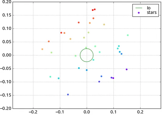
Figure 3.3: Io’s ellipsoid and stars’ direction projection on the focal plane

3.2.1 Ellipsoid projection

The algebraic process to obtain C, the projected ellipse matrix, was adapted from [22] and it starts from the ellipsoid matrix Q. This represents the equation of an ellipsoid in homogeneous coordinates, expressed in a reference frame which has the origin coincident with the center of the ellipsoid and the axes coincident with the principal axes of the ellipsoid (so that the frame is rotating with the celestial body): Q =      1/a2 ₀ ₀ ₀ 0 1/b2 ₀ ₀ 0 0 1/c2 ₀ 0 0 0 −1     

Where a, b and c are the principal semi-axes of the ellipsoid.

The first transformation applied to the ellipsoid matrix is a translation from the body-fixed frame to the camera frame. The translation vector ~trl is expressed

in the body-fixed frame and it is directed from the camera to the observed body. This translation transformation can be expressed in homogeneous matrix form as:

(22)

T =      1 0 0 trl[0] 0 1 0 trl[1] 0 0 1 trl[2] 0 0 0 1     

Where trl[0] , trl[1] and trl[2] are the first, second and third component of the translation vector ~trl 1_{. The translation is then applied as follows:}

Qt = T−TQT−1

The rotation from the body-fixed frame to the camera frame was split into two rotations passing from EMO2000 so that the overall rotation transformation can be written as: Qc= REC−TR −T BEQtR−1BER −1 EC

Where REC and RBE are 4x4 matrices representing the rotation from EMO2000 to the camera frame and the rotation from the body-fixed frame to EMO2000 respectively, in homogeneous coordinates.

The matrix Qc obtained after translation and rotation needs to be projected on the camera focal plane in order to obtain C. This is done multiplying for the intrinsic camera parameters matrix K:

K =    f 0 0 0 0 f 0 0 0 0 1 0   

Where f is the focal length, which is defined as the distance from the lens to the principal foci of the lens. The projection transformation is performed as follows:

C−1 = KQcKT

Here K is expressed as 3x4 matrix so that a 3x3 matrix (C−1) is obtained from a 4x4 matrix (Qc). Finally, the matrix has to be inverted to get the projected ellipse matrix C, in homogeneous coordinates.

3.2.2 Star direction projection

In order to obtain the star projection point on the camera focal plane, the star direction unit vector is normalized by its third component and projected using matrix Ks: ~x = Ksx~s_z1_s =    f 0 0 0 f 0 0 0 1       xs ys zs    1 zs

In this case, Ks is the intrinsic camera parameters matrix expressed as a 3x3 matrix, which is obtained omitting the fourth column of zeros in K.

(23)

3.2. GEOMETRICAL MODEL 11

3.2.3 2D distance

Initially, the geometric 2D distance between the moon’s ellipse and the star’s position point was considered. This approach allows the measurements to keep their physical meaning and maintain a direct connection to the real-life scenario. Although this was very useful to plot the stars’ distribution around Io and have an intuitive validation of the model, the architecture of the problem resulted to be quite inconvenient in order to compute the partial derivatives at a later stage.

For this reason, the algebraic distance was adopted instead. In this way the direct relation to the physical distance is lost, but the expression to be implemented is much easier:

h = ~xTC~x (3.1)

Where h is the ellipse-point distance, ~x is the star 2D position vector in homogeneous

coordinates and C is the projected ellipse matrix. This approach relies on the simple fact that when a point lays on the ellipse limbs it has to satisfy equation

h = ~xTC~x and thus h = 0. Analogously, h > 0 when the star is not occulted (i.e.

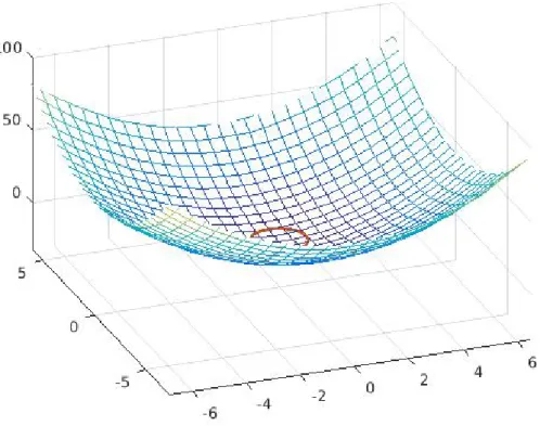
outside the ellipse area), and h < 0 when the star is occulted (i.e. inside the ellipse area). In this way, the beginning of a stellar occultation can be identified looking for the moment in which h turns from positive to negative, while the opposite is true for the end of the occultation. Figure 3.4 provides a visual confirmation of the distribution of h in the surroundings of the projected ellipse.

The integral code written to detect all the stellar occultations taking place in a given time span can be found in Appendix A.2.

Figure 3.4: 3D behavior of h as a function of the distance from the projected ellipse (red line)

(24)

3.3 Model implementation

Hereafter the salient parts of the code developed to compute the 2D distance between Io and the surrounding stars will be briefly commented in order to show how the models and the techniques presented above have been applied in practice. All the referenced codes can be found in A.1.

One of the main simplifications adopted throughout this work is that the camera frame is always pointing towards Io. Indeed, the frame is defined by two direction vectors: one refers to the Z axis, which is always pointing from JUICE to Io, and the other defines the XY plane reference direction and points from JUICE to Jupiter. This simplification allows to detect all the potential occultations and implement the optical parameters at a later stage. In order to find a stellar occultation, the first thing to do is to investigate which stars can be found in the background around Io at the time of interest, as seen from JUICE. Thus a star catalog needs to be loaded and then used as a database containing all the useful information regarding a given set of stars, such as their position, magnitude, parallax and spectral type. For this work, the UCACT-PI star catalog was adopted. It results from the merge of UCAC2 and Tycho-2 catalogs, but with parallax information from Hipparcos and magnitudes corrections for Cassini’s clear filter.

Using MONTE it is possible to obtain a list of all the stars which lay inside a given search circle centered around a given direction vector. In this case, the direction of interest was the one from JUICE to Io and the radius adopted for the search circle 10 deg. The minimum value for the stars’ apparent magnitude was set to −2 since there are no brighter stars in the catalog anyway, while the maximum was set to 6 to ensure the stars were bright enough to be detected by UVS. In order to determine the distance between Io’s limbs and each star around it, the moon’s ellipsoid projection has to be computed following the procedure detailed in Section 3.2.1.

Finally, iterating over the number of stars detected in the surroundings of Io, the star direction projection is computed and the distance between the moon’s ellipse and the star point is obtained.

(25)

Chapter 4 Partial derivatives

After having defined a suitable model for the stellar occultation events, one has to understand which are the main parameters affecting the chosen observable. In fact, this is the information conveyed by the partial derivatives: in which measure is

h influenced by the variation of the each parameter? Some of these parameters are

of interest and we want to estimate them, so the partials represent the sensitivity of the measurements to these parameters. Others are just an input, not to be estimated, and the partials represent the influence of an error in their knowledge on the measurements.

In this case, the first step consisted in identifying all the variables involved and then include the ones worth considering (i.e. which have a relevant influence on the observable). This was one of the most critical and complex parts of the work. Since the model for the observable h had been designed from scratch, there was no immediate reference as to the influence that other parameters have on it. After a preliminary selection, 11 parameters were included in the partial derivatives analysis:

• The star position, expressed as right ascension and declination;

• The shape of Io, expressed as the three semi-major axis defining the moon’s ellipsoid;

• The 3-dimensional position of Io; • The 3-dimensional position of JUICE;

Other parameters, such as the focal length f , the coordinate system rotations and the spacecraft’s attitude, were first considered and then discarded due to their limited (or null) influence on the problem, as it will be explained in the following sections.

In order to validate the results of the calculations, both the numerical and the algebraic partial derivatives were computed and then compared. Numerical partials may be affected by numerical errors but they are more straightforward to obtain, so that they can be easily used as a first reference to double-check the algebraic ones.

(26)

4.1 Algebraic Partials

Table 4.1 contains the equations of the partial derivatives of h with respect to all the aforementioned parameters. To derive the expression of the algebraic partials, one has to go back and start from equation (3.1). Differentiating the equation of h with respect to a generic scalar parameter q leads to the following expression:

∂h ∂q = ∂~xT ∂q C~x + ~x T∂C ∂q~x + ~x T_C∂~x ∂q

Since the first and the third term on the right hand side are scalars, they can be summed up to obtain: ∂h ∂q = 2~x T_C∂~x ∂q + ~x T∂C ∂q~x (4.1)

As can be seen from equation (4.1), the right hand side is made up by two main components: the first one contains the partial derivative of the star 2D position on the focal plane x with respect to q, while the second contains the partial derivative of the projected ellipse matrix C with respect to q.

4.1.1 Ellipse matrix derivative

From section 3.2.1, one can retrieve the expression of matrix C as a function of

Qc, which becomes: C = (Cinv)−1 = (KQ−1c K T₎−1 So that: ∂C ∂q = ∂(Cinv)−1 ∂q (4.2)

Recalling the formulation for the matrix inverse derivative B.1, equation (4.2) can be expressed as: ∂C ∂q = ∂(Cinv)−1 ∂q = −(Cinv) −1∂Cinv ∂q (Cinv) −1 = = −C∂(KQ −1 c KT) ∂q C = −C( ∂K ∂q Q −1 c K T _{+ K}∂Q −1 c ∂q K T _{+ KQ}−1 c ∂KT ∂q )C

And applying again (B.1) to Qc in the middle term of the right hand side:

∂C ∂q = −C( ∂K ∂q Q −1 c K T _{+ KQ}−1 c ∂Qc ∂q Q −1 c K T _{+ KQ}−1 c ∂KT ∂q )C

So that the computation of the partial derivative of C reduces to the computation of the partial derivative of K and Qc.

As shown in section 3.2.1, matrix K is a function of f only. It can be demon-strated that the focal length does not affect the observable h. In fact, both the projected ellipse and the star position point are scaled by f and its contribution cancels out when the terms are multiplied for each other in (4.1). This means that

∂K

(27)

4.1. ALGEBRAIC PARTIALS 15 The full expression for matrix Qc can be retrieved from section 3.2.1 as follows:

Qc= R−TECR

−T

BET

−T

QT−1R−1_BER_EC−1 (4.3) Now, one has to evaluate the partial derivative of Qc with respect to each one of the parameters. Looking at equation (4.3) and at the expression of the matrices

REC, RBE and T in section 3.2.1, it is clear that Qc is not affected by the star’s position coordinates. In fact, only a, b and c, the semi-major axis of Io’s ellipsoid, and trl[0], trl[1] and trl[2], the coordinates defining Io’s position in the body-fixed frame with respect to the camera, appear in the equation.

For the first triplet of parameters we obtain:

∂Qc ∂q = R −T ECR −T BET −T∂Q ∂qT −1 R−1_BER−1_EC

Where ∂Q_∂q becomes for a, b and c respectively:

∂Q ∂a =      −2/a3 _{0 0 0} 0 0 0 0 0 0 0 0 0 0 0 0      ∂Q ∂b =      0 0 0 0 0 −2/b3 _{0 0} 0 0 0 0 0 0 0 0      ∂Q ∂c =      0 0 0 0 0 0 0 0 0 0 −2/c3 ₀ 0 0 0 0     

The parameters defining Io’s position appear in the translation matrix only, so that the partial derivative of Qc becomes:

∂Qc ∂q = R −T ECR −T BE ∂T−T ∂q QT −1 R−1_BER−1_EC + R−T_ECR−T_BET−TQ∂T −1 ∂q R −1 BER −1 EC And once again using equation (B.1) one can write:

∂T−1

∂q = −T

−1∂T

∂qT

−1

Where ∂T_∂q for x = trl[0], y = trl[1] and z = trl[2] can be written as:

∂T ∂x =      0 0 0 1 0 0 0 0 0 0 0 0 0 0 0 0     

(28)

∂T ∂y =      0 0 0 0 0 0 0 1 0 0 0 0 0 0 0 0      ∂T ∂z =      0 0 0 0 0 0 0 0 0 0 0 1 0 0 0 0     

The partials derivatives with respect to JUICE’s position can be obtain simply changing the sign of the derivatives calculated for Io’s translation. In fact, from a physical point of view, moving JUICE has the same and opposite effect on the translation vector as moving Io. Additionally, ∂T_∂q has to be rotated from Io body-fixed to EME2000 as JUICE’s position is expressed in the inertial frame.

In the first place also the six angles defining the rotation from the body-fixed frame to EMO2000 and the rotation from EMO2000 to the camera frame were considered. However, their influence on the problem was quite limited and their observability was deemed small enough to neglect them without major consequences. Similarly, the attitude of the spacecraft was first considered and then discarded. In fact, the orientation of JUICE affects both the ellipsoid projection and the star direction projection in the same way, so that in the end its effect vanishes.

4.1.2 Star vector derivative

From section 3.2.1, one can retrieve the expression for ~x and differentiate it with

respect to the generic scalar parameter q:

∂~x ∂q = ∂(K ~xs_z1_s) ∂q = ∂_z1 s ∂q K ~xs+ 1 zs ∂K ∂q x~s+ 1 zs K∂ ~xs ∂q

As explained in the previous paragraph, ∂K_∂q = 0 since matrix K is a function of f only. If ~xs is expressed as a function of the star’s right ascension (Ra) and declination (Dec) as follows:

~ xs =    cos(Ra)cos(Dec) sin(Ra)cos(Dec) sin(Dec)   

one can see that ~xs is a function of Ra and Dec while _z1_s is a function of Dec only. Thus, the derivative of ~x with respect to the right ascension becomes:

∂~x ∂Ra = 1 zsK    −sin(Ra)cos(Dec) cos(Ra)cos(Dec) 0   

While the derivative with respect to the star’s declination can be written as: ∂~x ∂Dec = − cos(Dec) z2 s K ~xs+ 1 zsK    −cos(Ra)sin(Dec) −sin(Ra)sin(Dec) cos(Dec)   

(29)

4.1. ALGEBRAIC PARTIALS 17 T able 4.1: Algebraic partial deriv ativ es recap P arameter Algebraic partial a ∂ h ∂ a = − ~x T C (K Q − 1 c R − T E C R − T B E T − T ∂ Q T _∂a − 1 R − 1 B E R − 1 E C Q − 1 c K T )C ~x b ∂ h _∂b = − ~x T C (K Q − 1 c R − T E C R − T B E T − T ∂ Q T _∂b − 1 R − 1 B E R − 1 E C Q − 1 c K T )C ~x c ∂ h ∂ c = − ~x T C (K Q − 1 c R − T E C R − T B E T − T ∂ Q T _∂c − 1 R − 1 B E R − 1 E C Q − 1 c K T )C ~x x ∂ h ∂ x = − ~x T C (R − T E C R − T B E (− T − 1 ∂ T ∂ x T − 1 ) T QT − 1 R − 1 B E R − 1 E C + R − T E C R − T B E T − T Q (− T − 1 ∂ T ∂ x T − 1 )R − 1 B E R − 1 E C )C ~x y ∂ h ∂ y = − ~x T C (R − T E C R − T B E (− T − 1 ∂ T ∂ y T − 1 ) T QT − 1 R − 1 B E R − 1 E C + R − T E C R − T B E T − T Q (− T − 1 ∂ T T _∂y − 1 )R − 1 B E R − 1 E C )C ~x z ∂ h ∂ z = − ~x T C (R − T E C R − T B E (− T − 1 ∂ T T _∂z − 1 ) T QT − 1 R − 1 B E R − 1 E C + R − T E C R − T B E T − T Q (− T − 1 ∂ T T _∂z − 1 )R − 1 B E R − 1 E C )C ~x xsc ∂ h ∂ x = ~x T C (R − T E C R − T B E (− T − 1 ∂ T ∂ xsc T − 1 ) T QT − 1 R − 1 B E R − 1 E C + R − T E C R − T B E T − T Q (− T − 1 ∂ T ∂ xsc T − 1 )R − 1 B E R − 1 E C )C ~x ysc ∂ h ∂ y = ~x T C (R − T E C R − T B E (− T − 1 ∂ T ∂ y sc T − 1 ) T QT − 1 R − 1 B E R − 1 E C + R − T E C R − T B E T − T Q (− T − 1 ∂ T ∂ y sc T − 1 )R − 1 B E R − 1 E C )C ~x zsc ∂ h ∂ z = ~x T C (R − T E C R − T B E (− T − 1 ∂ T ∂ z sc T − 1 ) T QT − 1 R − 1 B E R − 1 E C + R − T E C R − T B E T − T Q (− T − 1 ∂ T ∂ z sc T − 1 )R − 1 B E R − 1 E C )C ~x R a ∂ h ∂ R a = 2 ~x T C 1 K _zs ∂ ~xc ∂ R a D ec ∂ h ∂ D e c = − 2 ~x T C ( cos (D ec ) z 2 s K ~xs + 1 K _zs ∂ ~xc ∂ D ec )

(30)

4.2 Numerical Partials

The numerical partials were obtained imposing a given variation of one pa-rameter at the time and then applying the finite difference method to obtain the approximation of the partial derivative:

∂h

∂q ≈

h(q + ∆q) − h(q)

∆q (4.4)

Appendix A.3 reports the code section which computes the partial derivative of h with respect to the first ellipsoid semi-major axis a as an example of the implementation scheme adopted. First, ∆a has to be chosen and summed to the actual value of a, which is stored among the information regarding Io and its shape ’Io Ellipsoid’. Then C matrix is computed and given as an input to the function which returns the value of the perturbed observable hda for all the stars in the surroundings of Io. Finally, the partials associated with each star are obtained using equation (4.4). The values delivered by this code where compared to the ones obtained using the algebraic equations detailed in section 4.1 at the same time and for the same set of stars. The same procedure was iterated for all the other parameters.

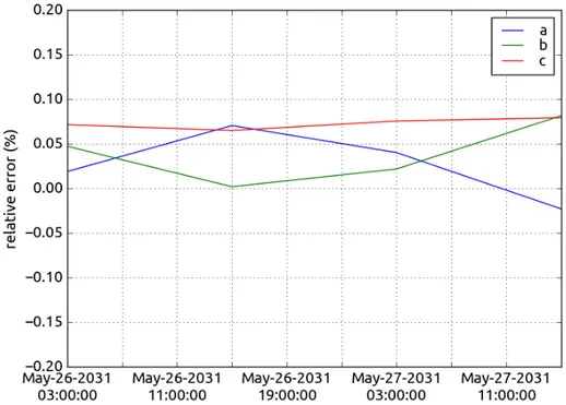
Figures 4.1, 4.2 and 4.3 show an example of visual validation of the partials derivatives for a single star on a 2-days time span. The relative error between algebraic and numerical partials was obtained as:

relative error = algebraic − numerical

numerical 100

Figure 4.1: Time evolution of the relative error associated to Io’s ellipsoid’s semi-major axis a, b, c

(31)

4.2. NUMERICAL PARTIALS 19

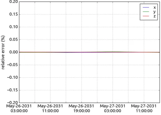
Figure 4.2: Time evolution of the relative error associated to the Io’s position coordinates x, y, z

Figure 4.3: Time evolution of the relative error associated to the star’s right ascension and declination

The validation was successfully completed as the magnitude of the relative error computed at different times and for different stars was found to be smaller than 0.2% for all the parameters of interest.

(32)

(33)

Chapter 5 Covariance Analysis

When confronting a new physical problem, one has to investigate which are the main parameters affecting the system and to what extent their misrepresentation can influence the outcome of the analysis. Generally, in a satellite orbit determi-nation problem two different kinds of parameters can be identified: measurement parameters and dynamic parameters. The former define the relationship between the satellite at a given time and an observation of the satellite at that same time. The latter affect the time evolution of the state of the satellite [18]. For example, in the stellar occultation problem treated here the JUICE spacecraft’s position is a measurement parameter, while the positions of the other Galilean moons are dynamic parameters. The standard deviation associated with one of the satellite’s state components results from the uncertainties on both measurement and dynamic parameters. The critical point is to understand which are the fundamental sources of ambiguity so that one knows where to focus in order to improve the estimation of the unknown quantities.

When evaluating the relevance of a parameter’s misrepresentation two factors have to be considered: what is the impact of the parameter’s inaccuracy on the estimation of the state of the satellite and how likely the parameter is to be misrepresented. The usual approach in this case is to develop a model of the physical problem at hand and obtain an estimation of the satellite’s state in nominal conditions. Subsequently, the same model is used to solve a new orbit determination problem in which the input value of the parameter being studied differs of what is believed to be the standard deviation of the parameter itself. The solutions delivered by the two settings are compared so that the time evolution of the effects of one sigma variation of the given parameter on the satellite’s state is obtained. Of course, this process can be quite expensive from a computational point of view. If this is the case, the Covariance Analysis can be an effective alternative to obtain (almost) the same results.

The Covariance Analysis consists in computing the state covariance matrix only, without actually estimating the state of the satellite. Using this technique one can obtain the standard deviation of the components of the state, which is the square root of the diagonal terms of the covariance matrix, and investigate how the uncertainty on each parameter influences the estimated uncertainty on the satellite’s state. However, the true error between the estimated state and the a priori state cannot be determined as the actual state estimation is not performed.

(34)

Usually, the true error is bigger than the standard deviation, so that the results of the Covariance Analysis tend to be optimistic and this is the main drawback related to this technique.

5.1 Variance, covariance and correlation

In general, the covariance matrix P associated to n estimated variables is a

n-dimensional squared symmetric matrix whose structure can be schematized as

follows: P =                σ2 1 σ12 · · · σ1i · · · σ1n σ12 σ22 · · · σ2i · · · σ2n .. . ... . .. ... ... σ1i σ2i · · · σ2i · · · σin .. . ... ... . .. ... σ1n σ2n · · · σin · · · σn2               

The elements on the diagonal correspond to the variance of each variable, which is the square of the standard deviation and for the generic i-th random variable X it is defined as:

σ_i2 = var(X) = E[(X − E[X])2] = cov(X, X)

Where E is the expectation operator and E[X] is the expected value of the variable

X. The off-diagonal elements represent the covariance of the variables, which is

a measure of their joint variability and for the generic i-th variable X and j-th variable Y it is defined as:

σij = cov(X, Y ) = E[(X − E[X])(Y − E[Y ])]

So the covariance matrix includes information regarding both the uncertainty associated to each variable and how each one is correlated with the others. In fact, one can also compute the correlation coefficient, which is a normalized form of the covariance and it can be easily extracted from matrix P as follows:

ρij = corr(X, Y ) =

cov(X, Y ) σiσj

= E[(X − E[X])(Y − E[Y ])]

σiσj

The correlation coefficient varies between 1 (i.e. perfect direct relationship between the variables, or correlation) and -1 (i.e. perfect inverse relationship between the variables, or anticorrelation). If the two variables considered are independent their correlation number is equal to zero and they are said to be "uncorrelated".

In order to have a visual and immediate indication of how the variables are influenced by each other, the correlation matrix can be computed and plotted. This appears as a large squared symmetric table where the color of the cells varies from white (no correlation, ρij = 0) to black (full correlation, |ρij| = 1) depending on the relationship between the corresponding variables. The correlation matrix for the stellar occultation problem treated here can be found in section ??.

(35)

5.2. COVARIANCE MATRIX DERIVATION 23

5.2 Covariance matrix derivation

The covariance matrix P is obtained using the following formulation:

P = (P₀−1+ ATW A)−1 (5.1)

Where P0 is the a priori covariance matrix, which contains the information regarding

the initial uncertainty of the parameters, A is the matrix containing the partial derivatives of the measured observable with respect to each one of the parameters and W is the weighting matrix. A qualitative analysis of this formula suggests that the covariance matrix relies both on the a priori knowledge of the system and on the contribution of the measurements. However, the measure in which these two kind of information are included in the calculation may vary. Indeed, if the initial uncertainty associated to the parameters is high, the contribution of P0 will be

lower since the a priori knowledge does not bear much information. Analogously, the function of the weighting matrix is to account for the accuracy and reliability of the measurements: if these are deemed to be a good source of information, their weights will be higher and their contribution more significant. On the other hand, if the uncertainty associated to measurements is too high, their weights will be lowered accordingly.

Hereafter the matrices appearing in (5.1) will be analyzed individually and their application to the stellar occultation problem will be illustrated.

5.2.1 Partial derivatives matrix

The function of matrix A is to bring into the estimation the new information associated to the measurements performed. In practice, if one has m measurements

~

z = (z1, z2, ..., zm) and n variables to be estimated ~x = (x1, x2, ..., xn), A is a (m, n)

matrix defined as:

A =           ∂z1 ∂x1 ∂z1 ∂x2 · · · ∂z1 ∂xn ∂z2 ∂x1 ∂z2 ∂x2 · · · ∂xn ∂xn .. . ... . .. ... ∂zm ∂x1 ∂zm ∂x2 · · · ∂zm ∂xn          

In the stellar occultation problem, the measurements correspond to the stellar occultations detected and selected throughout the JUICE mission. Originally, the distance h, modeled in section 3.2, was adopted as observable. However, this choice made the selection of the weighting coefficients of matrix W quite burdensome because of the non-direct physical meaning so in the end the observable was switched from the distance measurement h to the occultation time measurement t. The partial derivative associated to the new observable were easily obtained considering that when an occultation take place h(t, ~x) = 0 and thus1_:

dh d~x = ∂h ∂~x + ∂h ∂t ∂t ∂~x = 0

1_{here ~}_{x is the vector containing all the variables involved in the estimation, not the 2D distance}

(36)

∂t ∂~x = − ∂h ∂t !−1 ∂h ∂~x (5.2)

Where the term on the left hand side corresponds to the time partials, the first derivative on the right hand side was computed numerically, as outlined in 4.2, and the second are the distance partials.

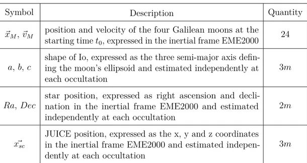
At this point, the variables to be included in the estimation had to be selected. After a few trials, the final choice included the parameters listed in Table 5.1. A part from the moons’ state, all the other parameters have been estimated independently at each occultation event. This adjustment allows to take into account the uncertainty associated to each variable in a simpler but less conservative way with respect to the consider parameters technique.

Table 5.1: Parameters included in the covariance analysis 2

Symbol Description Quantity

~xM, ~vM position and velocity of the four Galilean moons at the starting time t0, expressed in the inertial frame EME2000

24

a, b, c

shape of Io, expressed as the three semi-major axis defin-ing the moon’s ellipsoid and estimated independently at each occultation

3m

Ra, Dec

star position, expressed as right ascension and decli-nation in the inertial frame EME2000 and estimated independently at each occultation

2m

~ xsc

JUICE position, expressed as the x, y and z coordinates in the inertial frame EME2000 and estimated indepen-dently at each occultation

3m

5.2.1.1 Building the partial derivatives matrix

As mentioned above, each row of matrix A corresponds to one occultation, or more precisely to the time in which the occultation takes place, ti. The partials derivatives of ti with respect to the parameters a(ti), b(ti), c(ti), Ra(ti), Dec(ti),

xsc(ti), ysc(ti) and zsc(ti) had already been computed as shown in section 4.1. The partials with respect to the state of the moons at t0 was obtained using the chain

rule as follows: ∂ti ∂~xM(t0) = ∂ti ∂~xIO(ti) ∂~xIO(ti) ∂~xM(t0) (5.3) ∂ti ∂~vM(t0) = ∂ti ∂~xIO(ti) ∂~xIO(ti) ∂~vM(t0) (5.4) Where the subscript M indicates any of the moons Io, Europa, Ganymede or Callisto. Note that the i-th occultation time measurement is influenced directly by

(37)

5.2. COVARIANCE MATRIX DERIVATION 25 the position of Io, and in turn by the position and velocity of the other moons due to their gravitational influence on Io’s orbital evolution. From table 4.1 one can get:

∂h ∂~xIO(ti) = " ∂h ∂x, ∂h ∂y, ∂h ∂z # (5.5)

And then equation (5.2) can be used to switch from h to ti and obtain _∂~_x_IO(ti)∂ti . The terms ∂~_∂~x_xIO(ti)

M(t0) and

∂~xIO(ti)

∂~vM(t0) are usually referred to as "state transition matrix"

and they describes how the position of Io at time ti is influenced by the state of the Galilean moons (including Io itself) at the starting time t0.

5.2.1.2 Implementing the partial derivatives matrix

The state transition matrix was computed as a part of the orbit determination problem by integration of the variational equations. In this work the partials were obtained from the satellites’ partials ephemerides released by the JPL, thus assuming to use the same dynamical model. In particular, the state transition matrix was derived using MONTE’s method M.ParamList.transitionMatrix( Epoch t, ParamList q ). To do so, Io’s parameters of interest, ~xIO = (xIO, yIO, zIO), were declared as a ParamList, q_Io, and the state of all the moons was defined as a separate ParamList, q_moons. All the elements in q_Io have to be represented in Io body-fixed frame, to be consistent with the reference frame of the partials in (5.5), while the parameters in q_moons must be defined in EME2000, so that the resulting partial derivatives to be included in A are expressed in the inertial frame. Asking for q_Io.transitionMatrix( t_plot, q_moons ) returns the 3x24 transition matrix to be used in (5.3) and (5.4), selecting the terms relative to the moons’ position or velocity respectively.

5.2.2 Weighting matrix

Matrix W was introduced in formulation 5.1 to account for the reliability of the measurements, weighting each of them accordingly. In general, if m measurements are available, W is a m-dimensional squared diagonal matrix. It is common practice to assume the measurements noise to be un-correlated (white) and use the reciprocals of the variance associated to each measurement as diagonal entries, such that W results to be: W =         1 σ2 1 0 · · · 0 0 _σ12 2 · · · 0 .. . ... . .. ... 0 0 · · · 1 σ2 n        

In this way, the higher the variance (i.e. the uncertainty) associated to a measure-ment, the lower to corresponding weight and the smaller its contribution to the estimation process.

Having switched from the observable h to the time of the occultation t, the choice of the weights for the stellar occultation problem was quite straightforward.

(38)

In fact, the measurements timing accuracy is given by the characteristics of the UVS instrument and the on-board clock, so that W becomes:

W = 1

σ2

time

I

Where I is the identity matrix.

The time accuracy for JUICE is 1ms at best so that, in order to be conservative,

σtime = 5ms was chosen as nominal value.

5.2.3 A priori covariance matrix

The purpose of the a priori covariance matrix P0 is to include the contribution

of the current knowledge of the problem in the estimation. From a mathematical point of view, this is a way to obtain a reliable solution when the problem is not fully observable, such as when the measurements do not carry much information about some variables. This is the case, for example, the outer moons’ state.

As the name suggests, P0 has the same structure and characteristics as matrix

P , so section 5.1 can be taken as a reference. In this case, P0 was chosen to be a

diagonal matrix, thus excluding any a priori correlation between different variables. If n is the number of parameters included in the estimation, P0 is a n-dimensional

square diagonal matrix whose structure simplifies to:

P0 =           σ2 01 0 · · · 0 0 σ2 02 · · · 0 .. . ... . .. ... 0 0 · · · σ2 0n          

As shown by equation 5.1, the a priori covariance matrix has to inverted in order to obtain P . In this way, the higher the initial uncertainty of one parameter, the lower the diagonal element and the smaller the contribution of the a priori knowledge associated to that parameter.

5.2.3.1 Choice of the a priori standard deviation

The choice of the a priori σ0 values for the estimated parameters is a quite

delicate one. In principle, one can retrieve this information from the literature. However, the material is not always easily accessible. Additionally, the numerical effect of the a priori knowledge must be taken into account as well as the choice of

P0 has a relevant influence on the numerical stability of the problem.

So after many researches and a few tuning investigations, the final a priori values were selected as reported in table 5.2.

(39)

5.2. COVARIANCE MATRIX DERIVATION 27

Table 5.2: A priori standard deviations

Parameter σ0 Reference

Io initial position 50km [1]

Europa initial position 0.5km [1] Ganymede initial position 0.05km [1] Callisto initial position 0.5km [1] Moons initial velocity 0.0001km/s N/A

Io dimensions 6.3km [20]

stars position 10µas [19]

JUICE position 0.1km [21]

According to [1], the current uncertainty on the Galilean moon’s position is 5km in all the three radial, downtrack and out-of-plane directions. Yet, the a priori

σ0 on Io’s position was set to 50km not to constrain the estimation.

On the other hand, the accuracy on the other three Galilean moons’ position is likely to improve considerably. In fact, JUICE will orbit Ganymede for 8 months, gaining crucial information on the moons’ dynamics, so that it can be safely assumed that the satellite’s position uncertainty will decrease to 0.05km approximately. Analogously, since both JUICE and Europa Clipper will perform various flybys of Europa and Callisto, the uncertainty on the two moons’ position was reduced to 0.5km. Also, the values in [1] have been calculated propagating the moons’ trajectory from 1990 to 2020, which is a considerably long period of time, so the uncertainty is likely to be a bit overestimated if applied to a mission which lasts 2.5 years.

Unfortunately no reliable reference was found for the a priori moons’ velocity uncertainty so the value of 0.0001 km/s was chosen believing it to be a reasonable one.

The uncertainty on Io’s dimensions is related to the unevenness of its surface rather than to the precision of the ellipsoid semi-axes definition. In fact, the time of the occultation is affected by the actual morphology of Io’s surface, i.e. by the irregularity of its limbs as seen from the camera. Additionally, the uncertainty associated to the semi-axes of the ellipsoid shape is considerably lower than the average dimension of Io’s geographical features, so this approach is conservative anyway. Since the average elevation of the moon’s mountains is 6.3km, this value was taken as a priori σ0.

The stars’ position accuracy adopted is the one recently obtained thank to the GAIA mission. As stated in [19], the uncertainty on the location of the brightest

(40)

stars (i.e. whose apparent magnitude is lower than 12) varies between 5 and 16 µas. Since in this work only the stellar occultations of stars whose apparent magnitude is lower than 6 mag were considered, the a priori σ0 was taken to be equal to 10

µas, being conservative.

According to [21], the uncertainty associated to the JUICE spacecraft’s position will be 10 m in terms of formal error. So to adopt a conservative value for the a priori formal error, 0.1 km was chosen.

5.3 Covariance matrix propagation

Once the covariance matrix P has been computed, one knows what is the estimated uncertainty associated to each variable at the reference time. However, hardly ever the investigation is restricted to a singular time instant and so a tool to propagate the estimation in time is needed. Once again, the state transition matrix is used, just as in section 5.2.1.1, but this time it is applied through matrix multiplication as follows:

P (t) = Φ(t, t0)P (t0)Φ(t, t0)T

Where P (t0) is the covariance matrix calculated at the reference time t0, Φ(t, t0) is

the state transition matrix from t0 to the current time t, and P (t) is the covariance

matrix associated to time t.

The state transition matrix was provided by MONTE using the

M.ParamList.transitionMatrix( Epoch t, ParamList q ) method, as explained in section 5.2.1.1. The only difference is that in this case the ParamList q_Io is defined in Io’s RTN reference frame, so that the propagated covariance matrix is expressed in this frame and one does not need to manually rotate it. In fact, from a physical point of view, it is more meaningful to analize the position uncertainty in the radial, tangential and normal direction of the orbital reference frame.

(41)

Chapter 6 Results

Hereafter the results obtained from the Covariance Analysis will be discussed. The main aim of this investigation is to understand how the a priori knowledge of the estimated parameters and the selection of the stellar occultations affect the estimation of the position of the target moon, Io.

The analysis will start presenting the results of the Covariance Analysis for the nominal case, then a parametric analysis which highlights the influence of each parameter on the estimation will follow and in the end the effects of the number and distribution of the stellar occultation observations will be examined.

6.1 Nominal case analysis

For the nominal case 239 occultation events were considered, imposing a maxi-mum frequency of one observation every three days and a star apparent magnitude between -2 and 6 mag. The occultations available on ESA’s Cosmos website [23] were used as a loose reference for the scheduled number of stellar occultation events. As expected, the quantity of occultations detected by the code developed for this Thesis is considerably higher that the one foreseen by ESA, even excluding the observations disturbed by other celestial bodies. This is due to the fact that the simplified camera frame used here assumes that UVS is always pointing towards Io, thus detecting more occultations than the actual instrument would.

The time interval considered throughout the analysis coincides with JUICE’s 2.5 years tour of the Jovian system (January 2030 - June 2033). The only difference is that instead of including also the very first orbital phase after the Jupiter Orbit Insertion (JOI), it was chosen to set the beginning of the investigation in April 2030 so to limit the maximum distance between Juice and Io and deal with more regular orbits, as can be seen in Figure 6.1. Looking at the graph, it is clear that, even if the occultations have been selected to be no closer that three days from each other, the distribution of the measurements is not uniform. In fact, in the last phase of the mission, when JUICE will be orbiting Ganymede, the occultations are denser with respect to the first period. A clear indication of this unevenness is that the time interval considered here goes from 20th _{April 2030 to 26}th _{June 2033, so that}

the middle value falls on 22th _{November 2031, while the (239/2)}th _{occultation takes}

place on 27th _{March 2032. This means that roughly the 62% of the occultations is}

(42)

detected in the second half of the mission.

Improvement of Jupiter's satellites ephemerides using stellar occultation observations

Alma Mater Studiorum

Università di Bologna

School of Engineering

Forlì Campus

Master’s Degree in Aerospace Engineering

Class LM-20

Graduation Thesis in:

Spacecraft Orbit Determination and Control

Improvement of Jupiter’s

satellites ephemerides using

stellar occultation observations

Candidate:

Francesca Andreoli

Supervisor:

Prof. Marco Zannoni

III session

Abstract

Contents

List of Figures

List of Tables

Chapter 1

Acronyms

Chapter 2

Introduction

2.1

The Jovian system

2.2

The Laplace resonance

2.3

The JUICE mission

2.4

MONTE

Chapter 3

Stellar occultations model

3.1

Stellar occultations

3.2

Geometrical model

3.2.1

Ellipsoid projection

3.2.2

Star direction projection

3.2.3

2D distance

3.3

Model implementation

Chapter 4

Partial derivatives

4.1

Algebraic Partials

4.1.1

Ellipse matrix derivative

4.1.2

Star vector derivative

4.2

Numerical Partials

Chapter 5

Covariance Analysis

5.1

Variance, covariance and correlation

5.2

Covariance matrix derivation

5.2.1

Partial derivatives matrix

5.2.2

Weighting matrix

5.2.3

A priori covariance matrix

5.3

Covariance matrix propagation

Chapter 6

Results

6.1

Nominal case analysis